Author Contributions
Conceptualization, P.d.P.M., E.Y.A. and Á.N.d.S.; methodology and validation, P.d.P.M., E.Y.A., Á.N.d.S. and R.S.P.; formal analysis, P.d.P.M., E.Y.A., R.M.C., F.E., Á.N.d.S., R.S.P. and E.A.T.M.; investigation and data curation, P.d.P.M., R.M.C., E.Y.A., F.E., Á.N.d.S., R.S.P., E.A.T.M. and E.P.M.; writing—preparation of original draft, P.d.P.M.; writing—review and editing, P.d.P.M., Á.N.d.S., E.Y.A. and E.A.T.M. All authors have read and agreed to the published version of the manuscript.
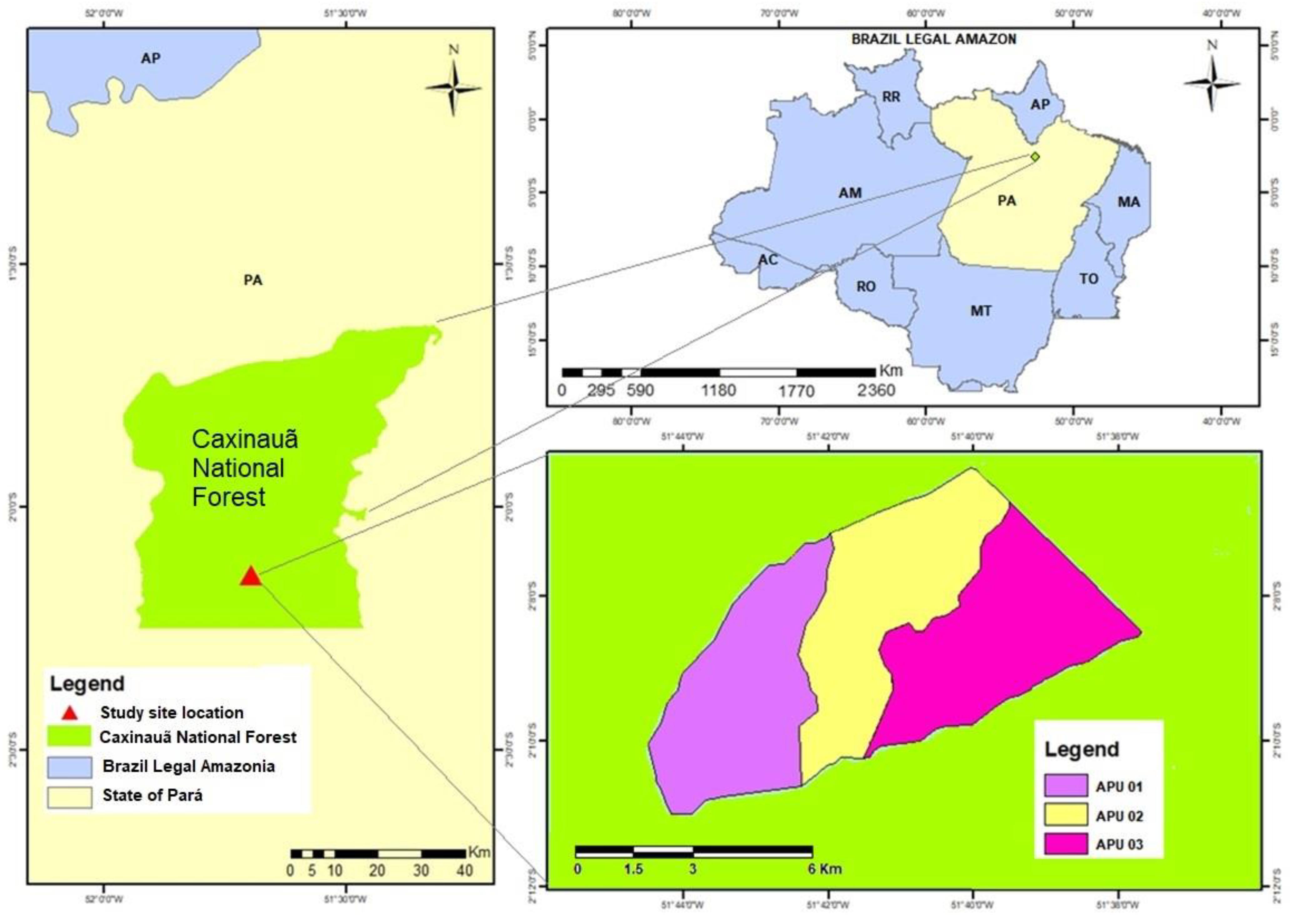
Figure 1.
The study site is situated within the Caxiuanã National Forest, located in the state of Pará, Brazil. It includes three Annual Production Units (APUs) within the forest concession area, which were granted to the CEMAL timber company by the Brazilian Forest Service.
Figure 1.
The study site is situated within the Caxiuanã National Forest, located in the state of Pará, Brazil. It includes three Annual Production Units (APUs) within the forest concession area, which were granted to the CEMAL timber company by the Brazilian Forest Service.
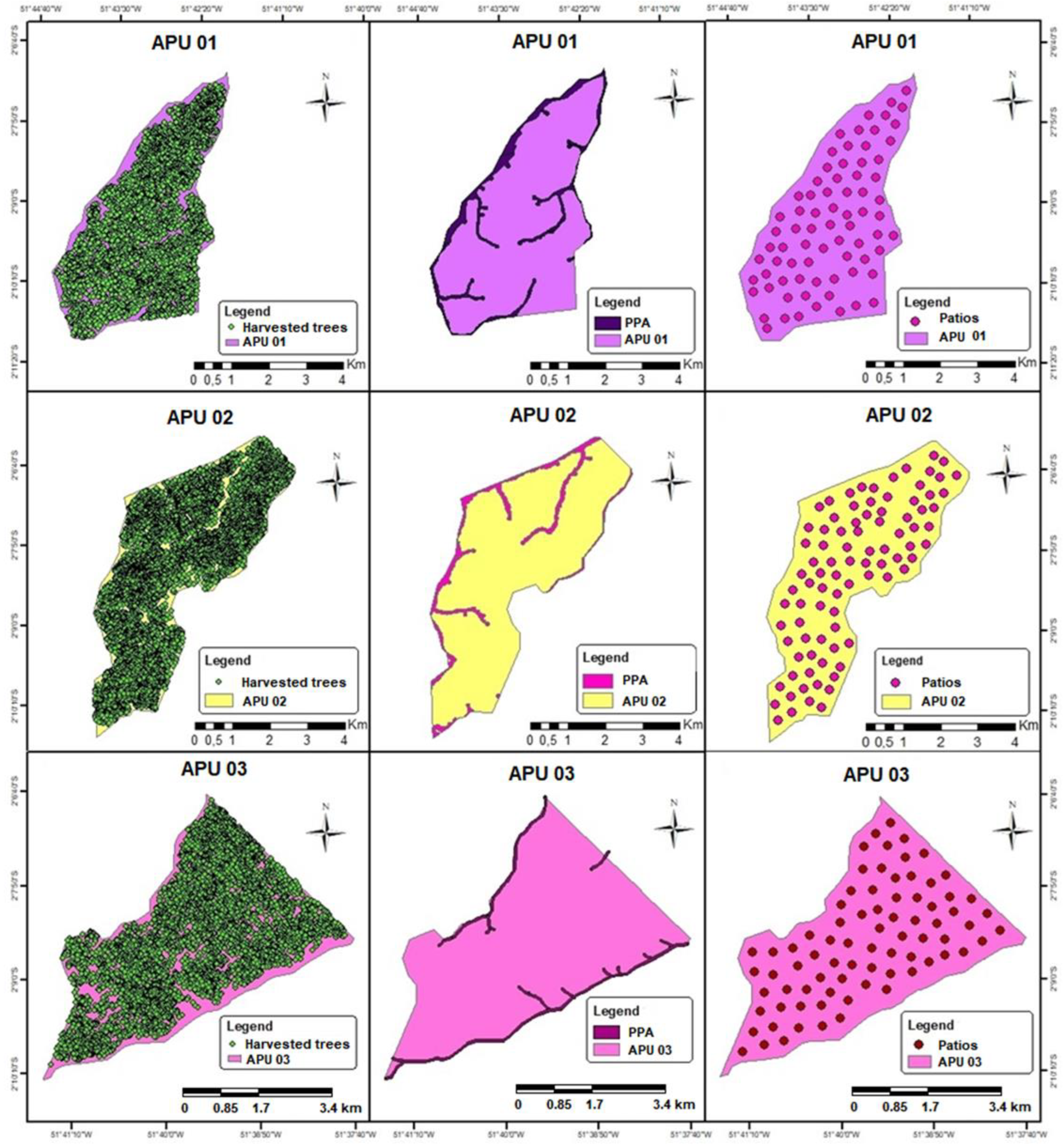
Figure 2.
Spatial location of the logged trees, the Permanent Protected Areas (PPA), and the log-landings within each Annual Production Unit (APU) in the study site.
Figure 2.
Spatial location of the logged trees, the Permanent Protected Areas (PPA), and the log-landings within each Annual Production Unit (APU) in the study site.
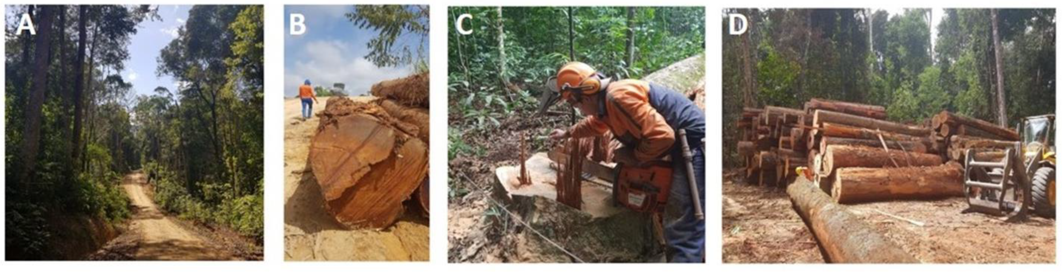
Figure 3.
(
A) Forest road; (
B) trees dragged from the forest; (
C) a tree trunk just after felling; and (
D) a log-storage patio in the Caxiuanã National Forest, state of Pará, Brazil. Photos were taken in 2019 and provided by [
27].
Figure 3.
(
A) Forest road; (
B) trees dragged from the forest; (
C) a tree trunk just after felling; and (
D) a log-storage patio in the Caxiuanã National Forest, state of Pará, Brazil. Photos were taken in 2019 and provided by [
27].
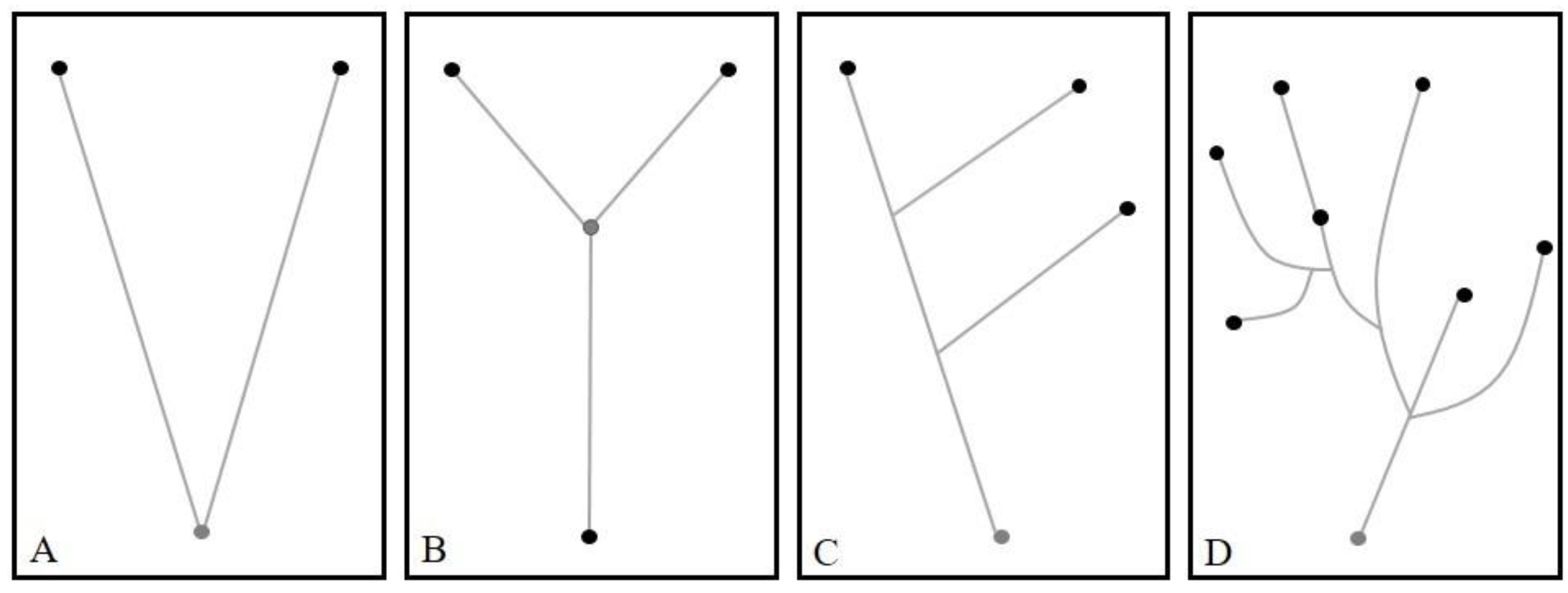
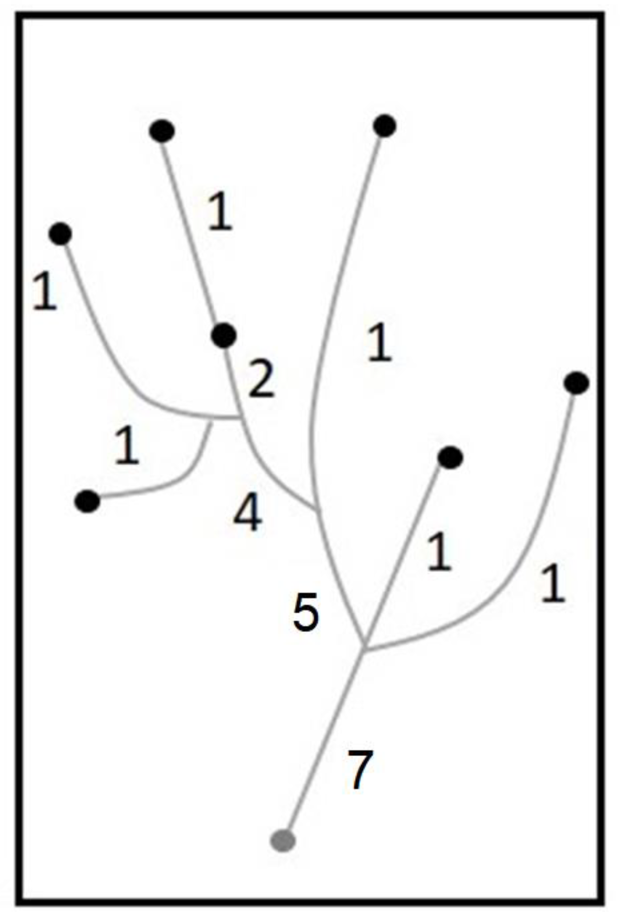
Figure 4.
Different ways to connect dots: (A) solution found (Least Cost Path) in most of Geographic Information Systems; (B) Global Model; (C) Minimum Spanning Tree approach; and (D) Tomlin approach.
Figure 4.
Different ways to connect dots: (A) solution found (Least Cost Path) in most of Geographic Information Systems; (B) Global Model; (C) Minimum Spanning Tree approach; and (D) Tomlin approach.
Figure 5.
Tomlin Modeling (adapted from [
21]) shows the frequency of log transportation on each forest road segment.
Figure 5.
Tomlin Modeling (adapted from [
21]) shows the frequency of log transportation on each forest road segment.
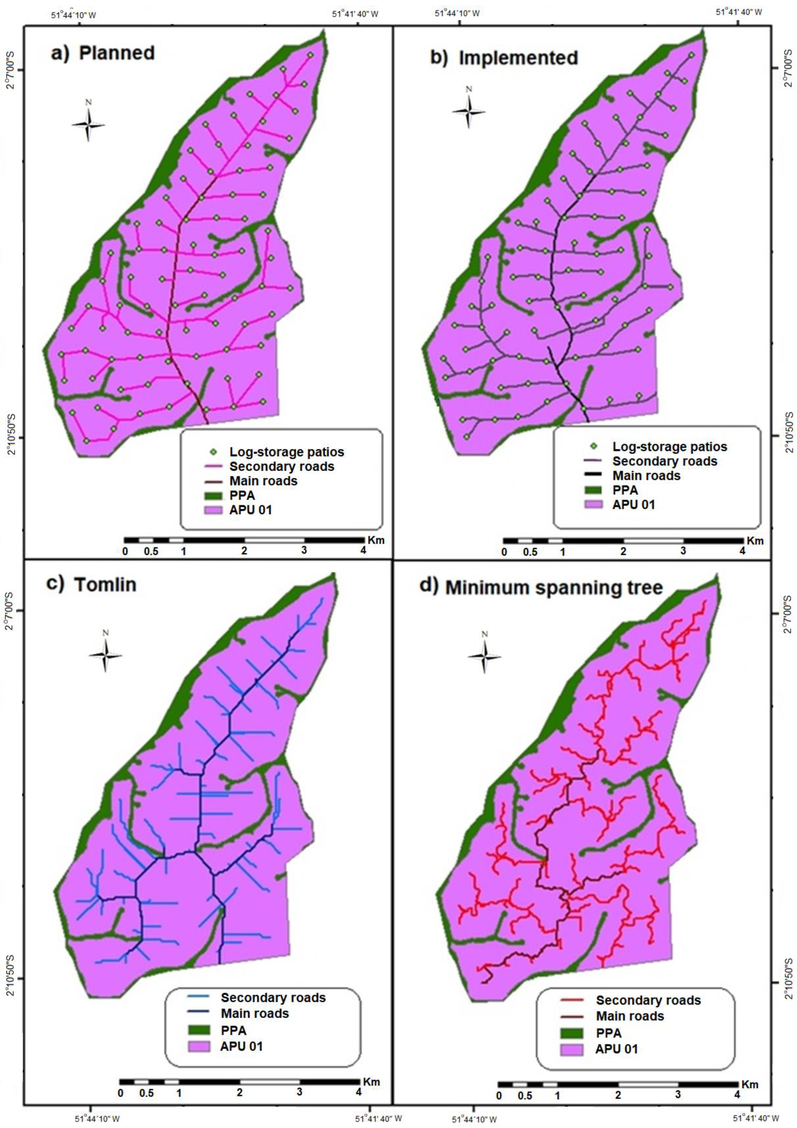
Figure 6.
Annual Production Unit (APU) 01: (a) planned roads (main and secondary roads) and log-landings; (b) implemented roads (main roads, secondary roads) and log-landings; (c) modelled roads using the TOMLIN modeling approach with Tobler´s hiking cost, including main and secondary roads; (d) modelled roads using the Minimum Spanning Tree with Dheight friction cost, including mains and secondary roads. PPA = Permanent Protected Areas in which selective logging activities are not allowed and APU = Annual Production Unit, an area.
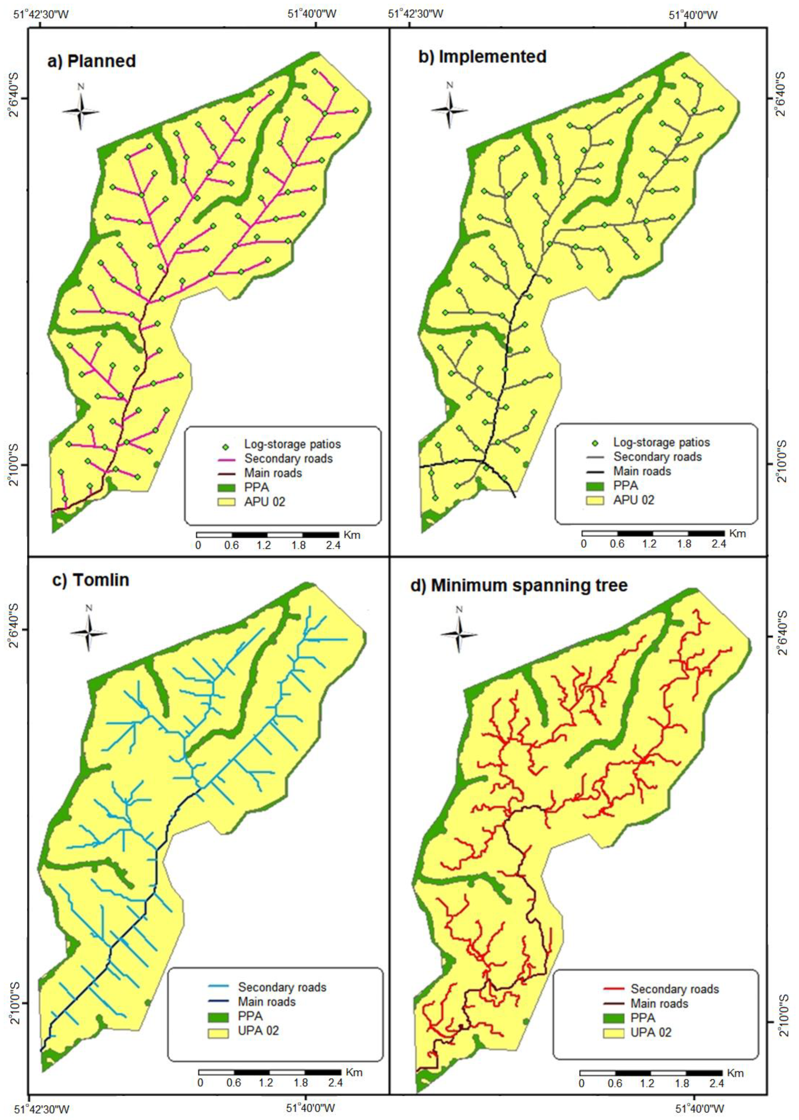
Figure 7.
Annual Production Unit (APU) 02: (a) planned roads (main road, country road, and planned log-storage patios); (b) roads executed (main road, secondary road, and executed). (c) Roads delineated by Model 1 (TOMLIN) contain main roads and secondary roads. (d) Roads modelled by Model 2 (Minimum Spanning Tree) contain main roads and secondary roads.
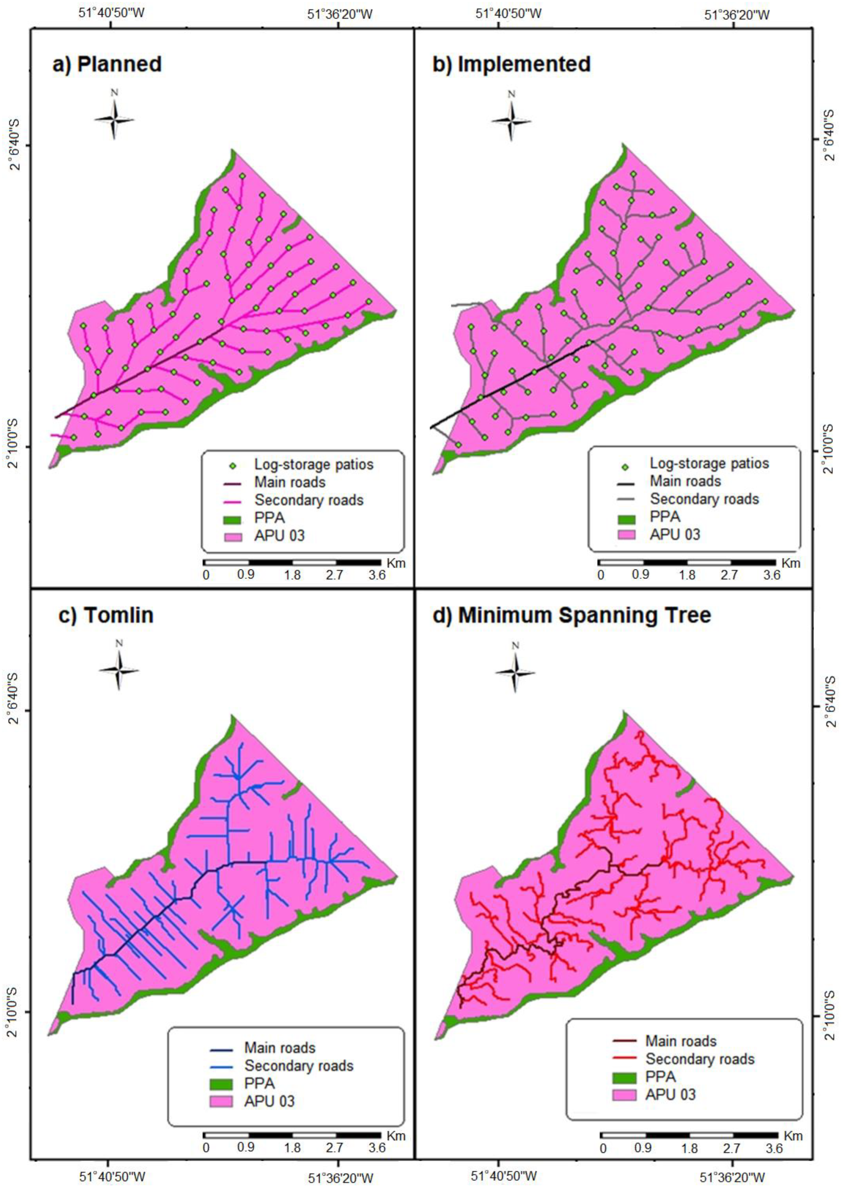
Figure 8.
Annual Production Unit (APU) 03: (a) planned roads (main road, secondary road, and planned patios); (b) roads executed (main road, secondary road, and executed). (c) Roads delineated by Model 1 (TOMLIN) contain main road and secondary roads. (d) Roads modelled by Model 2 (Minimum Spanning Tree) contain main roads and secondary roads.
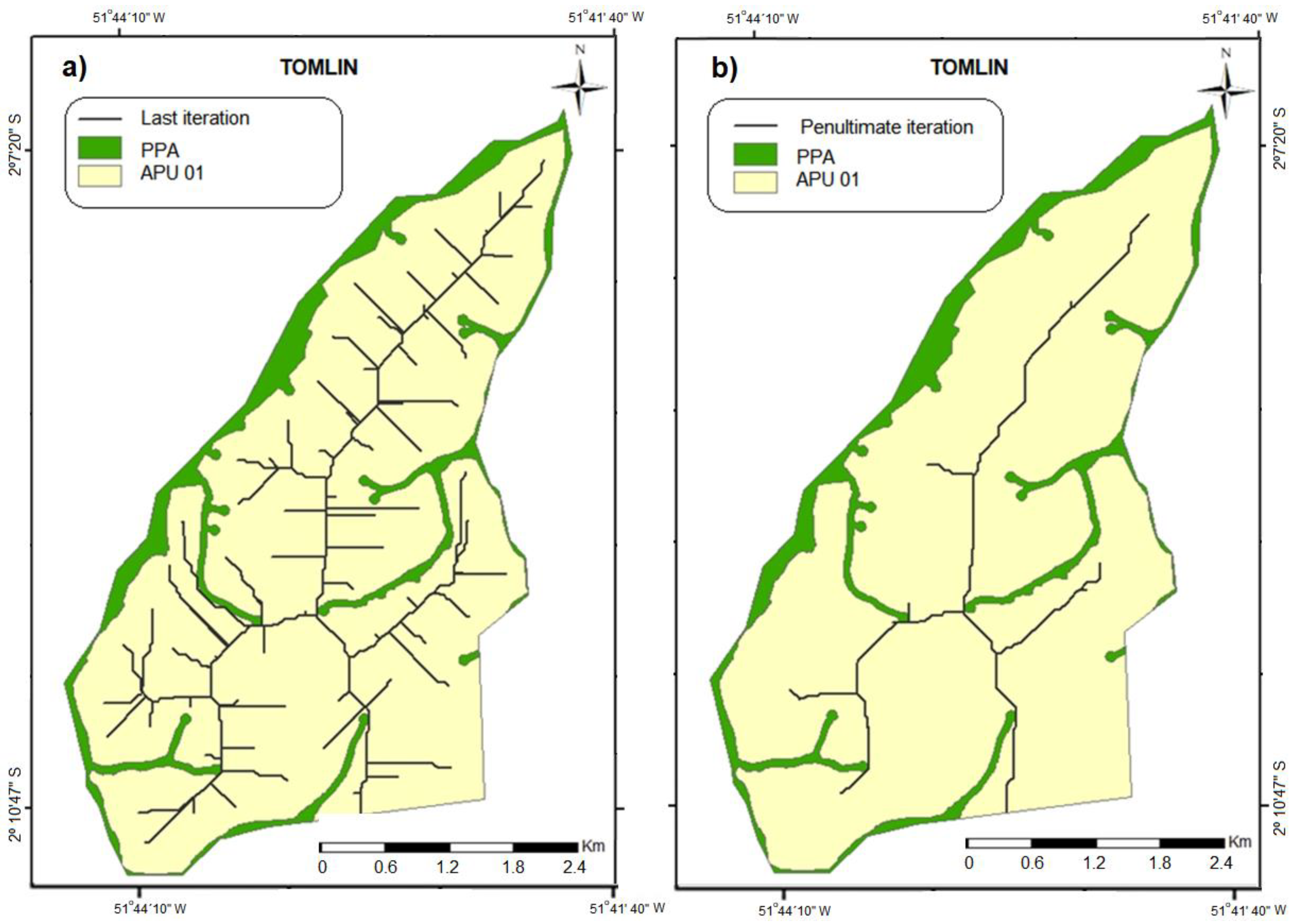
Figure 9.
(a) Tomlin modeling with last iteration and (b) the Tomlin modeling with the penultimate iteration.
Figure 9.
(a) Tomlin modeling with last iteration and (b) the Tomlin modeling with the penultimate iteration.
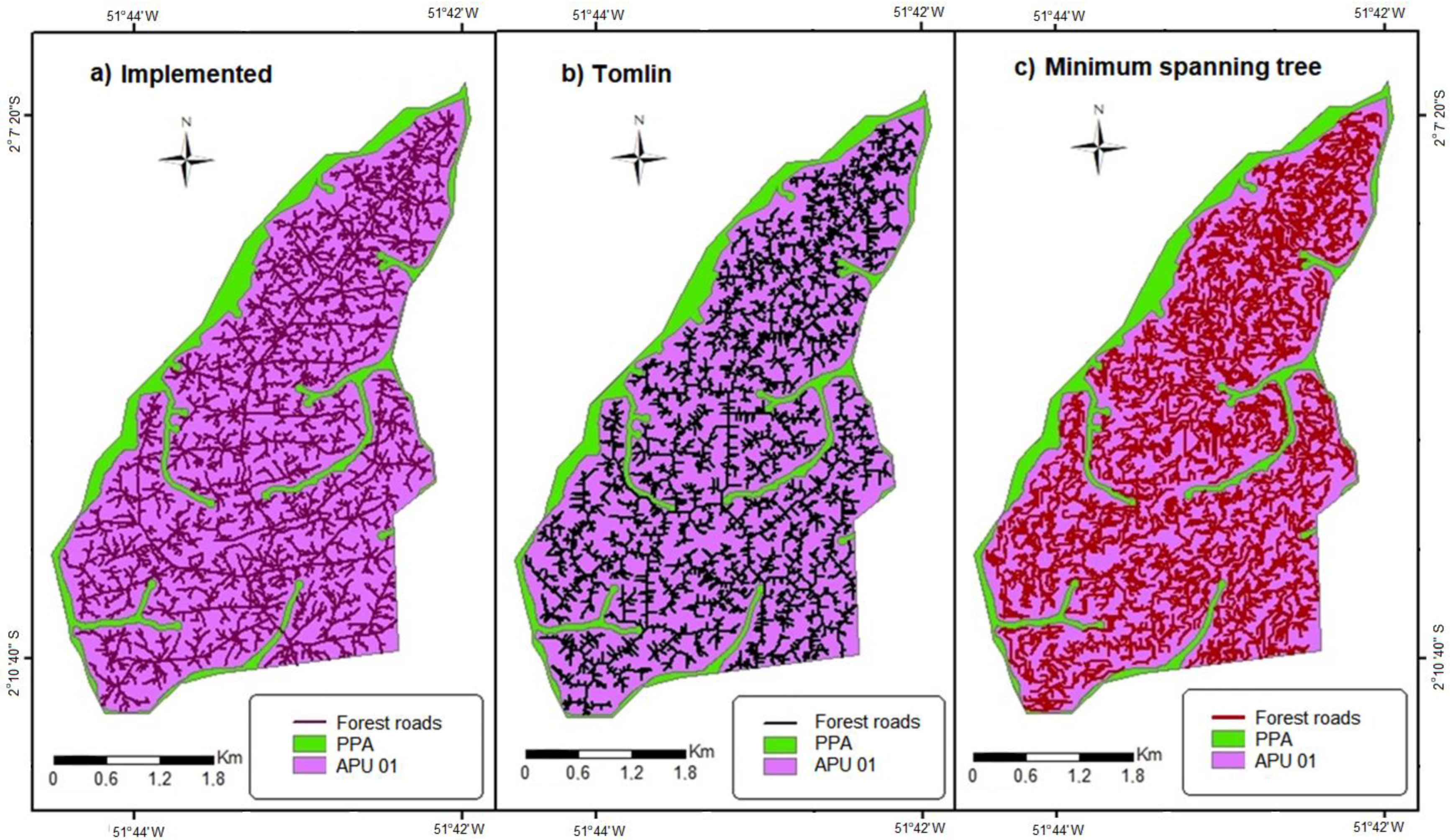
Figure 10.
APU 01: (a) logging infrastructure implemented by CEMAL Ltd.; (b) road design by applying Model 1 (TOMLIN) and (c) Model2 (Minimum Spanning Tree).
Figure 10.
APU 01: (a) logging infrastructure implemented by CEMAL Ltd.; (b) road design by applying Model 1 (TOMLIN) and (c) Model2 (Minimum Spanning Tree).
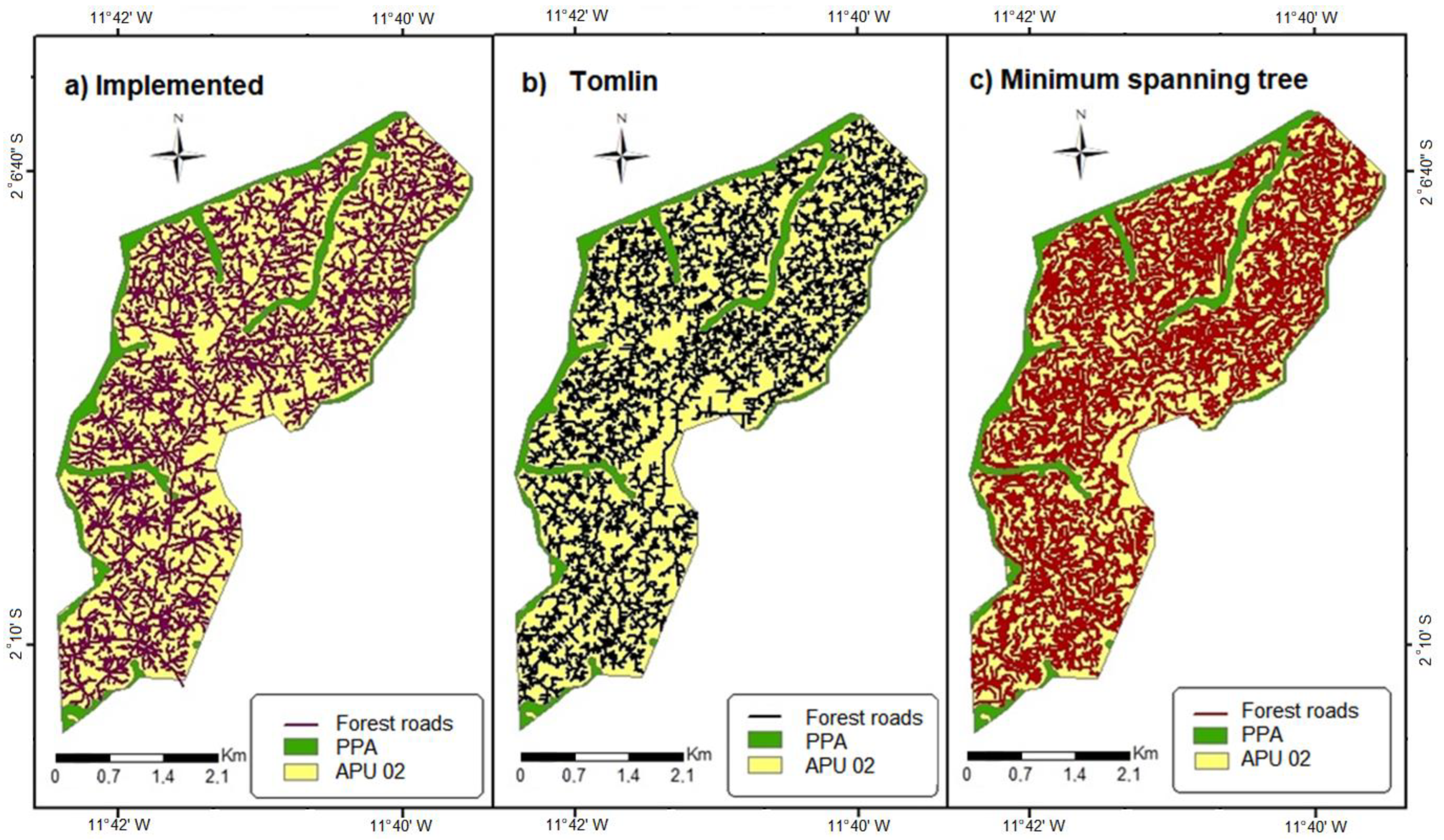
Figure 11.
APU 02: (a) logging infrastructure implemented by CEMAL Ltd.; (b) road design by applying Model 1 (TOMLIN) and (c) Model2 (Minimum Spanning Tree).
Figure 11.
APU 02: (a) logging infrastructure implemented by CEMAL Ltd.; (b) road design by applying Model 1 (TOMLIN) and (c) Model2 (Minimum Spanning Tree).
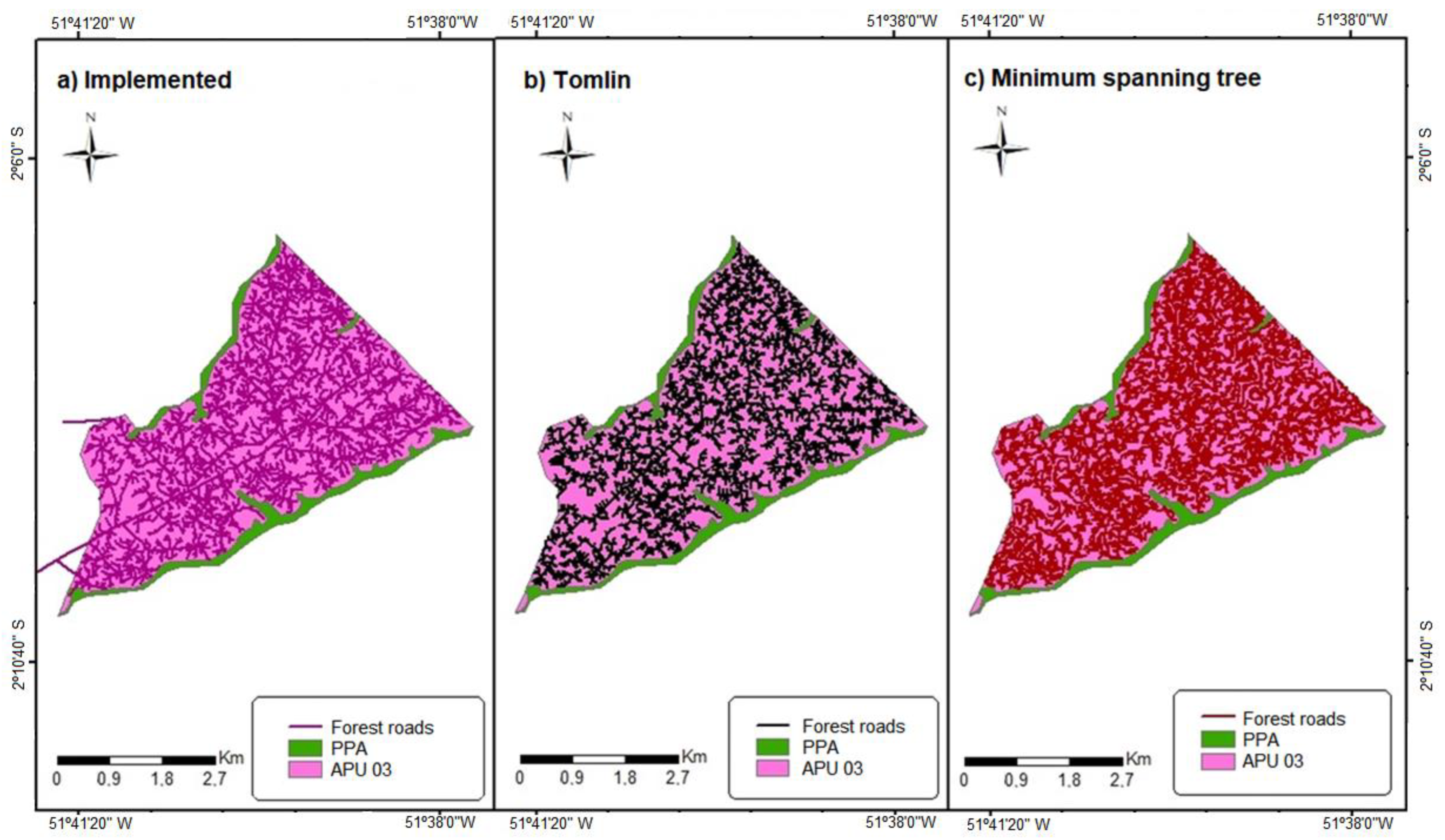
Figure 12.
APU 03: (a) logging infrastructure implemented by CEMAL Ltd.; (b) road design by applying Model 1 (TOMLIN) and (c) Model2 (Minimum Spanning Tree).
Figure 12.
APU 03: (a) logging infrastructure implemented by CEMAL Ltd.; (b) road design by applying Model 1 (TOMLIN) and (c) Model2 (Minimum Spanning Tree).
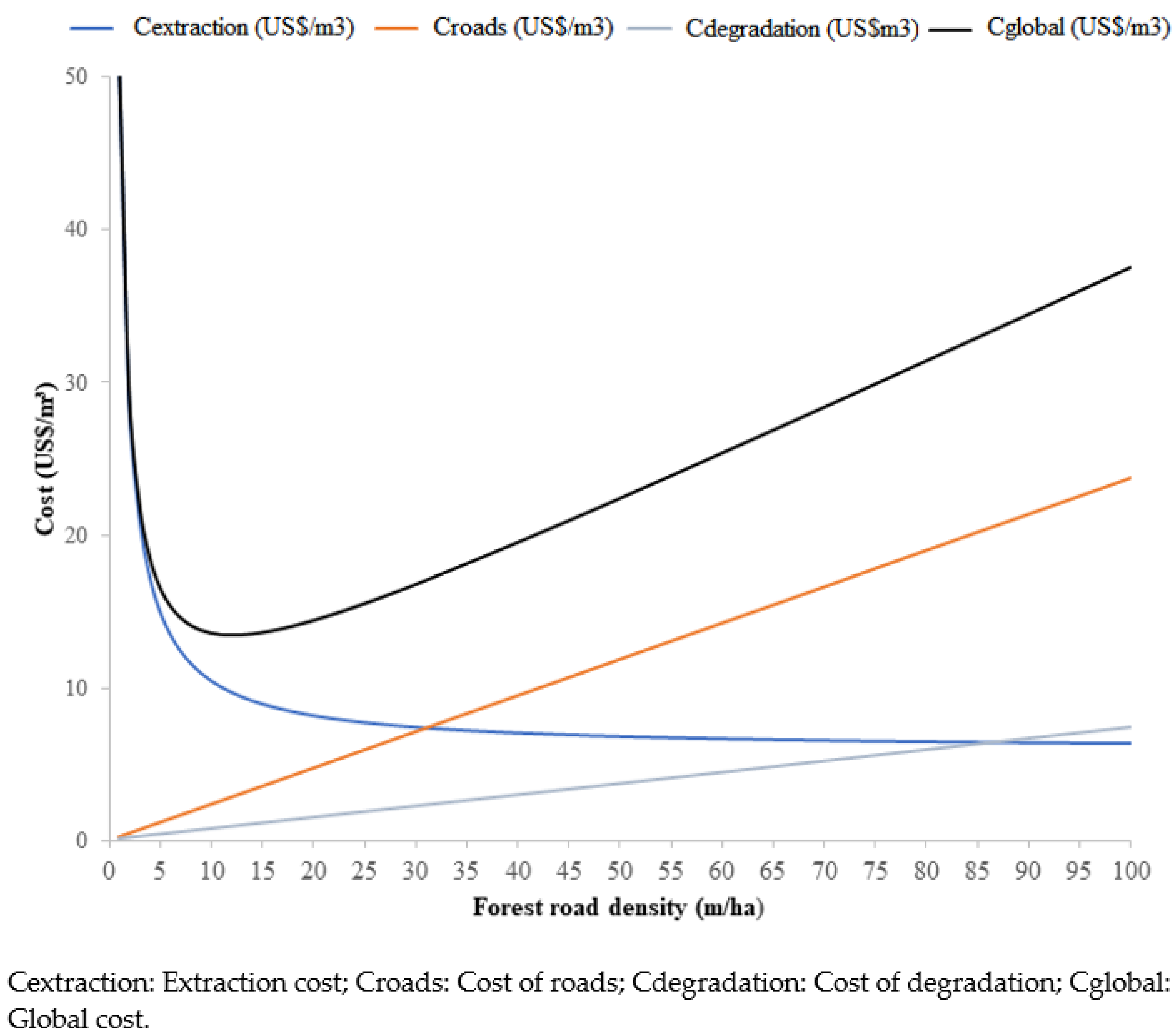
Figure 13.
Relationship between road density and road costs, extraction and degradation costs, and loss of productive forest area in a clear-cutting system.
Figure 13.
Relationship between road density and road costs, extraction and degradation costs, and loss of productive forest area in a clear-cutting system.
Table 1.
Annual Production Units (APU) in the study site within the Caxiuanã National Forest, state of Pará, Brazil.
Table 1.
Annual Production Units (APU) in the study site within the Caxiuanã National Forest, state of Pará, Brazil.
| Annual Production Unit (*) | Area (ha) | Harvesting Year |
|---|
| 1 | 1828.5 | 2019 |
| 2 | 1951.9 | 2020 |
| 3 | 1949.1 | 2021 |
| Total | 5729.5 | |
Table 2.
Skidding log dataset.
Table 2.
Skidding log dataset.
| Skidding Log | Skidder Costs |
|---|
| Extracted logs per day * | 5.00 | Acquisition price (USD) * | 386,220.00 |
| Average log volume (m3) * | 2.5 | Resale value (USD) ** | 77,243.20 |
| Working hours per day * | 8.00 | Estimate lifespan (year) ** | 25.00 |
* Dataset provided by [27]
** Data from current scientific literature | Fuel consumption (L·h−1) * | 14.00 |
| Diesel price (USD/L) | 1.35 |
| Hydraulic oil consumption (L·h−1) ** | 0.21 |
| Hydraulic oil price (USD/L) | 6.76 |
| Motor oil consumption (L·h−1) ** | 0.13 |
| Motor oil price (USD/L) | 3.28 |
| Tire price (USD/unit) ** | 2793.10 |
| Tire lifespan (hour)** | 2500.00 |
| Wage (USD/months) ** | 391.60 |
Table 3.
Total area of main roads and secondary roads in each Annual Production Unit (APU), the number of bridges, and the impacted areas on Permanent Protected Areas (PPA).
Table 3.
Total area of main roads and secondary roads in each Annual Production Unit (APU), the number of bridges, and the impacted areas on Permanent Protected Areas (PPA).
| APU * | Models | Area (Hectares) | Bridges |
|---|
| Main Roads | Secondary Roads | Impacted PPA ** |
|---|
| 01 | Planned | 7.32 | 27.41 | 0.11 | 1 |
| Implemented | 8.14 | 25.41 | 0.10 | 1 |
| Tomlin | 12.09 | 26.62 | 0 | 0 |
| Minimum Spanning tree | 14.14 | 32.20 | 0 | 0 |
| 02 | Planned | 7.99 | 30.11 | 0 | 0 |
| Implemented | 8.54 | 26.50 | 0.15 | 1 |
| Tomlin | 8.77 | 30.24 | 0 | 0 |
| Minimum Spanning tree | 13.45 | 39.89 | 0 | 0 |
| 03 | Planned | 6.22 | 29.60 | 0 | 0 |
| Implemented | 6.77 | 29.52 | 0 | 0 |
| Tomlin | 8.99 | 33.23 | 0 | 0 |
| Minimum Spanning tree | 15.04 | 39.86 | 0 | 0 |
Table 4.
The total length of roads and skid trails.
Table 4.
The total length of roads and skid trails.
| APU * | Total Length of Roads and Skid Trails (Meters) |
|---|
| Field-Implemented | Tomlin | Minimum Spanning Tree |
|---|
| 01 | 232,640.1 | 249,376.7 | 431,715.2 |
| 02 | 286,268.0 | 324,140.0 | 564,977.3 |
| 03 | 266,895.6 | 283,017.1 | 498,923.0 |
Table 5.
APU 01: costs of selective logging, roads, environmental degradation, total cost, road density, average road density, and spacing between secondary roads with the current values, in addition to the optimum and acceptable values for each variable.
Table 5.
APU 01: costs of selective logging, roads, environmental degradation, total cost, road density, average road density, and spacing between secondary roads with the current values, in addition to the optimum and acceptable values for each variable.
| Modeling Approach | Cext | Croad | Cdeg | CTot | RD | ASD | RS |
|---|
| USD m−3 | m.ha−1 | m | m |
|---|
| Planned | 8.33 | 4.48 | 1.40 | 14.21 | 18.83 | 248.94 | 573.15 |
| Field-implemented | 8.52 | 4.16 | 1.30 | 13.98 | 17.48 | 268.16 | 607.03 |
| Tomlin model | 8.38 | 4.40 | 1.37 | 14.15 | 18.47 | 253.79 | 589.41 |
| Spanning tree model | 7.93 | 5.36 | 1.67 | 14.97 | 22.51 | 208.24 | 589.41 |
| Optimum | 9.68 | 2.89 | 0.90 | 13.47 | 12.11 | 386.98 | 825.37 |
| Acceptable | 8.39 | 4.38 | 1.37 | 14.14 | 18.41 | 254.62 | 543.18 |
Table 6.
APU 02: costs of selective logging, roads, environmental degradation, total cost, road density, average road density, and spacing between secondary roads with the current values, in addition to the optimum and acceptable values for each variable.
Table 6.
APU 02: costs of selective logging, roads, environmental degradation, total cost, road density, average road density, and spacing between secondary roads with the current values, in addition to the optimum and acceptable values for each variable.
| Modeling Approach | Cext | Croad | Cdeg | CTot | RD | ASD | RS |
|---|
| USD m−3 | m·ha−1 | m | m |
|---|
| Planned | 8.27 | 4.61 | 1.44 | 14.32 | 19.36 | 242.12 | 569.21 |
| Field-implemented | 8.59 | 4.06 | 1.27 | 13.91 | 17.05 | 274.93 | 589.41 |
| Tomlin model | 8.25 | 4.65 | 1.45 | 14.34 | 19.51 | 240.26 | 597.75 |
| Spanning tree model | 7.66 | 6.20 | 1.93 | 15.79 | 26.03 | 180.08 | 597.75 |
| Optimum | 9.68 | 2.89 | 0.90 | 13.47 | 12.11 | 386.98 | 825.37 |
| Acceptable | 8.39 | 4.38 | 1.37 | 14.14 | 18.41 | 254.62 | 543.18 |
Table 7.
APU 03: costs of selective logging, roads, environmental degradation, total cost, road density, average road density, and spacing between secondary roads with the current values, in addition to the optimum and acceptable values for each variable.
Table 7.
APU 03: costs of selective logging, roads, environmental degradation, total cost, road density, average road density, and spacing between secondary roads with the current values, in addition to the optimum and acceptable values for each variable.
| Modeling Approach | Cext | Croad | Cdeg | CTot | RD | ASD | RS |
|---|
| | USD m−3 | m·ha−1 | m | m |
|---|
| Planned | 8.30 | 4.54 | 1.42 | 14.26 | 19.06 | 245.93 | 732.39 |
| Field-implemented | 8.31 | 4.52 | 1.41 | 14.25 | 19.00 | 246.71 | 1190.97 |
| Tomlin model | 8.00 | 5.18 | 1.62 | 14.81 | 21.77 | 215.32 | 960.47 |
| Spanning tree model | 7.66 | 6.18 | 1.93 | 15.78 | 25.97 | 180.5 | 960.49 |
| Optimum | 9.68 | 2.89 | 0.90 | 13.47 | 12.11 | 386.98 | 825.37 |
| Acceptable | 8.39 | 4.38 | 1.37 | 14.14 | 18.41 | 254.62 | 543.18 |


 ,
, 


