Article

3PG-MT-LSTM: A Hybrid Model under Biomass Compatibility Constraints for the Prediction of Long-Term Forest Growth to Support Sustainable Management

1
School of Information Science and Technology, Beijing Forestry University, Beijing 100083, China
2
Engineering Research Center for Forestry-Oriented Intelligent Information Processing, National Forestry and Grassland Administration, Beijing 100083, China
3
Research Institute of Forestry Informatization, Beijing Forestry University, Beijing 100083, China
*
Author to whom correspondence should be addressed.
Forests 2023, 14(7), 1482; https://doi.org/10.3390/f14071482
Submission received: 27 June 2023 / Revised: 14 July 2023 / Accepted: 18 July 2023 / Published: 19 July 2023
(This article belongs to the Special Issue Modeling Forest Response to Climate Change)

Abstract

:
Climate change is posing new challenges to forestry management practices. Thinning reduces competitive pressure in the forest by repeatedly reducing the tree density of forest stands, thereby increasing the productivity of plantations. Considering the impact of thinning on vegetation and physiological and ecological traits, for this study, we used Norway spruce (Picea abies) data from three sites in the PROFOUND dataset to parameterize the 3-PG model in stages. The calibrated 3-PG model was used to simulate the stand diameter at breast height and the stem, root, and leaf biomass data on a monthly scale. The 3PG-MT-LSTM model uses 3-PG simulation data as the input variable. The model uses a long short-term memory neural network (LSTM) as a shared layer and introduces multi-task learning (MTL). Based on the compatibility rules, the interpretability of the model was further improved. The models were trained using single-site and multi-site data, respectively, and multiple indicators were used to evaluate the model accuracy and generalization ability. Our preliminary results show that, compared with the process model and LSTM algorithm without MTL and compatibility rules, the hybrid model has higher biomass simulation accuracy and shows a more realistic biomass response to environmental driving factors. To illustrate the potential applicability of the model, we applied light (10%), moderate (20%), and heavy thinning (30%) at intervals of 10, 15, 20, 25, 30 years. Then, we used three climate scenarios—SSP1-2.6, SSP2-4.5, and SSP5-8.5—to simulate the growth of Norway spruce. The hybrid model can effectively capture the impact of climate change and artificial management on stand growth. In terms of climate, temperature and solar radiation are the most important factors affecting forest growth, and under warm conditions, the positive significance of forest management is more obvious. In terms of forest management practices, less frequent light-to-moderate thinning can contribute more to the increase in forest carbon sink potential; high-intensity thinning can support large-diameter timber production. In summary, moderate thinning should be carried out every 10 years in the young-aged forest stage. It is also advisable to perform light thinning procedures after the forest has progressed into a middle-aged forest stage. This allows for a better trade-off of the growth relationship between stand yield and diameter at breast height (DBH). The physical constraint-based hybrid modeling approach is a practical and effective tool. It can be used to measure long-term dynamic changes in forest production and then guide management activities such as thinning to achieve sustainable forest management.

1. Introduction

Forests are the main part of terrestrial ecosystems and also the largest carbon storage pool on land [1,2,3]. Human-induced climate change could fundamentally alter forests in the 21st century, with profound implications for the world [4]. Forest biomass is a key indicator in global carbon cycle research [5]. Thinning is a common forestry management practice. It has a significant and direct impact on forest structure. The understory microclimate will change with the change of structure and then affect the growth and development of trees [6,7]. Through thinning, stand density is reduced, the interception of precipitation is decreased while the understory light level is increased, and the decomposition of forest litter is accelerated [8]. Retained wood can make full use of light, water, and soil, and forest productivity can finally be improved. Accurately estimating the synergistic effect of thinning and climate on forest growth is of great significance for optimizing the utilization of forest resources and improving the ecological quality of forests [9,10,11]. In recent years, researchers have extensively explored how to estimate the response of forest biomass to thinning operations and climate change [12,13].
With the in-depth study of forestry management, mechanistic models have been developed and have received more and more attention [14,15]. A process model can simulate the key mechanistic processes of photosynthesis, respiration, and carbon water balance in tree growth. A process model takes into account the impact of climate factors and human disturbance on forest growth [16]. Individual-tree process models such as MAESTRA or TRIPLEX are established based on the three-dimensional spatial information of a single tree. These models take into account the extent to which the canopy utilizes solar radiation [17,18]. Individual-tree process models exhibit a high level of precision in their simulations. However, individual-tree process models rely on field surveys, which can incur higher costs. A stand process model, such as 3-PG or FORECAST, considers the effects of stand structure, climate change, and management practices. This model effectively elucidates and simulates the influence of environmental variables on the growth of forests [19,20]. Ecosystem process models, such as BIOME-BGC or LPG-DGVM, have comprehensively incorporated the carbon cycle within the atmosphere-vegetation-soil system. Its complexity is higher, and it is more suitable for large-scale carbon-water cycle simulation [21,22]. The essence of the process model is to complete the description of the material exchange and energy flow processes between the atmosphere, vegetation, and soil with the help of complex empirical equations. However, due to the fact that the environment is everchanging and will continue to change in the future, a model established based on past knowledge may no longer hold true. Therefore, it is difficult to predict dynamic changes in forests on a long-term scale (e.g., 50a).
With the development of artificial intelligence technology, Deep Learning (DL) provides a new means for forecasting forest growth and harvest [23,24]. DL does not restrict the selection of data sources. It is able to automatically extract knowledge from data streams to provide more flexible predictions. Kraft et al. [25] used LSTM to build a global model for fitting the Normalized Difference Vegetation Index (NDVI). Their model shows that LSTM can identify the memory effect of vegetation state on climate with satisfactory fitting accuracy. In addition to LSTM, other DL methods are also widely used. Neto et al. [26] used principal component analysis (PCA) to reduce the dimensionality of input data and used an Artificial Neural Network (ANN) to estimate productivity dynamics during Eucalyptus rotations. With a limited sample size, it shows better results than other forest productivity estimation methods. Xu et al. [27] proposed a neural network model with a multi-task loss function. This model solves the compatibility problem of tree biomass estimation and improves the generalization ability of the model. Despite the numerous successes of the DL model, its limitations are also evident [28,29,30]. First of all, the accuracy and generalization ability of the model depend on the ‘feeding’ of large amounts of data. However, the collection of forestry data requires a lot of effort and material resources. The process is also cumbersome and expensive. Secondly, the quality of the collected data cannot be guaranteed during the data collection process. There may be noise present in the data. Additionally, the training of the model can be disrupted, producing completely incorrect results. Thirdly, the training process of DL models does not involve any physical mechanisms. This can lead to unreasonable simulations in certain scientific problems.
Building hybrid interpretable models is currently a very active research frontier [31,32]. The hybrid model combines the physical consistency of process models and the high data-driven performance of DL methods [30]. Reichstein et al. [32] summarized the feasible avenues for coupling physical models with DL in geoscience problems. Among them, coupling strategies have been developed in the processes of runoff prediction and biological regulation [33,34]. Coupling physical processes into the loss function of neural networks enables more seamless hybrid model building [35]. However, the increase in interpretable components may generate more errors, resulting in a decrease in system performance. Therefore, the key to hybrid modelling is to explore the optimal solution to the “accuracy versus transparency trade-off” problem [36,37].
In the context of climate change, precisely assessing the impact of thinning on forest growth presents a viable approach to enhance forest structure, ecological quality, and service functions [12,38]. At present, we still lack the technical means to effectively and accurately understand how management behaviors affect forest production. The objectives of this manuscript were to: (1) Take the 3-PG simulation value as the model input variable, construct a 3PG-MT-LSTM hybrid model to increase model interpretability, sensitivity to thinning events, and the accuracy of long-term biomass predictions. (2) Introduce biomass compatibility rules to ensure that the model converges to a solution that follows the basic physical laws, further improving the generalization ability of the model, and evaluate the multi-index accuracy of the optimized model. (3) Under the conditions of multi-climate scenarios, estimate the impact of different thinning practice intervals and intensities on the growth of Norway spruce.

2. Materials and Methods

In this study, environmental elements, stand biomass observations, and geographic location information were first obtained from the PROFOUND database [39] (https://doi.org/10.5880/PIK.2020.006, accessed on 12 December 2022). The study area biomass data information is shown in Section 2.1. Then, we used the 3-PG model to amplify the original biomass observation data at different time intervals into monthly scale data. The 3PG-MT-LSTM model was established based on the biomass compatibility rule, using 3-PG simulated values as model inputs. Based on the characteristics of monthly average temperature, carbon dioxide concentration, monthly frost days, monthly average solar radiation, monthly precipitation, and monthly average water vapor pressure difference, the model realizes the prediction n of the forest stand stem, root, foliage, aboveground, and total biomass, and DBH. Using the single-site model as a basis, the factors of elevation, slope, and aspect were added to construct a multi-site model. The specific experimental method is presented in Section 2.2. In Section 2.3, we evaluate the accuracy of single-site and multi-site models using multiple evaluation metrics. According to the evaluation results, the model is continuously adjusted and optimized. Subsequently, in conjuction with CMIP6 multi-model and multi-scenario climate data (https://esgf-node.llnl.gov/projects/cmip6/, accessed on 14 February 2023), we simulate the growth of Norway spruce at the Bily Kriz site under different thinning regimes in Section 2.4. Finally, also in this paper, according to the simulation results, we analyze the impact of thinning on Norway spruce growth and make recommendations for forest management. The research framework is shown in Figure 1.

2.1. Norway Spruce Biomass Data

Norway spruce is a large, fast-growing, and highly adaptable evergreen coniferous tree species commonly used as a timber tree throughout Europe. The growth rate of Norway spruce is at its peak between 20 and 90 years. After 90 years, the rate gradually slows down. In this study, the biomass data of Norway spruce and historical meteorological data were obtained from the PROFOUND database (Table 1).

2.2. The 3PG-MT-LSTM Hybrid Modelling Approach

2.2.1. 3-PG Model

The 3-PG (Physiological Principles in Predicting Growth) model is a process-based model that simulates forest growth and yield with a monthly time scale [19]. It is widely used for predicting biomass production and carbon sequestration in forest ecosystems. The model uses environmental variables such as temperature, precipitation, and solar radiation to predict forest growth. The model illustrates key physiological and ecological processes such as photosynthesis, respiration, and nutrient cycles in forest production. The key process formulation of the model is shown in Equation (1).
G P P = α C x × F P A R × P A R × f T × f N × f F × f a g e × m i n f V P D ,   f S W
Among them, G P P refers to the gross primary productivity of forest stands; α C x refers to the quantum efficiency of the vegetation canopy, which is the number of CO2 molecules assimilated by vegetation per absorbed light quantum; F P A R (Fraction of photosynthetically active radiation absorption) refers to the proportion of photosynthetically active radiation absorbed by vegetation; P A R (Photosynthetically active radiation) refers to the radiation that drives photosynthesis; and f T , f N , f F , f a g e , and f V P D represent the correction factors for temperature, soil fertility, frost, stand age, vapor pressure deficit, and soil moisture, respectively.
Compared with other models, the 3-PG model is relatively simple to use and requires fewer input parameters. In addition, the model is available in multiple open-source versions such as EXCEL [40], Python [41], and R. We followed the method of 3-PG and used the ‘r3pg’ package of R program [42] to estimate biomass [43]. In this study, we used the Morris method to analyze the sensitivity of physiological and ecological parameters involved in the 3-PG model. The Morris sensitivity analysis method facilitates a global sensitivity analysis of parameters by calculating model outputs by changing only one input value between successive simulation runs [44]. Considering that forest growth is a dynamic process, we re-fitted and optimized the model parameters (i.e., phased localization model) after the thinning events and changes in the structure of the stand age groups. Finally, we used the built-in biomass allocation module in the 3-PG model to simulate the allocation of stand biomass among leaves, stems, and roots. The estimated values were used as inputs for the multi-task LSTM.

2.2.2. Multi-Task Learning and LSTM

MTL (Multi-task learning) is a machine learning technique that enables the joint training of multiple related tasks [45,46]. In this study, MLT is used to jointly predict the individual organ and total biomass changes in forest stands. LSTM is a type of recurrent neural network that can process sequential data by selectively remembering or forgetting past information [47,48]. The key process in LSTM is mathematically shown below.
f t = σ g W f x t + W f m t 1 + b f
i t = σ g W i x t + W i m t 1 + b i
o t = σ g W o x t + W o m t 1 + b o
c t = f t c t 1 + i t σ c W c x t + W c h t 1 + b c
m t = o t σ h c t
From Equation (2) to Equation (6), σ g , σ c , and σ h represent logistic sigmoid function, the input activation function, and the output activation function, respectively. f , i , o , and c represent the forget gate, input gate, output gate and cell activation vector, respectively. m depicts the hidden state vector, also known as output vector, of the LSTM units. W denotes the weight matrix (for example, W i represents the weight matrix of input gate). The stands for element-wise multiplication, and b denotes the bias term.
For this study, LSTM was used to model the temporal dynamics of biomass change. The combination of multi-task learning and LSTM allows the model to capture the complex relationships between thinning rules and climate change. By sharing the LSTM layer and jointly training the model on multiple related tasks, the MT-LSTM model can learn to generalize better and make more accurate predictions [49,50].

2.2.3. Loss Function

In this study, the loss function used in the MT-LSTM model consists of mean squared error (MSE) loss function and biomass compatibility rules. MSE loss function is defined as the average of squared differences between the actual and the predicted value (Equation (7)). In the MT-LSTM model, stem ( y s t e m ), root ( y r o o t ), leaf biomass ( y l e a f ), aboveground biomass ( y a b o v e g r o u n d ), and total biomass ( y t o t a l ) were all estimated independently. The addition of biomass correlation ensures the compatibility of the model, which is important for accurate biomass estimation. The rule is based on the principle of mass balance, which states that the total biomass in the system must always be consistent with the sum of the components. The following equations (Equations (8) and (9)) are the biomass correlation rules added to the loss function:
M S E = 1 n i = 1 n ( y i _ t r u e y i _ p r e d i c t i o n ) 2
y t o t a l = y a b o v e g r o u n d + y r o o t
y a b o v e g r o u n d = y s t e m + y l e a f
In Equation (7), n is the number of samples, while y i _ t r u e and y i _ p r e d i c t i o n are the observed value of the i th sample and its corresponding predicted value, respectively. y t o t a l , y a b o v e g r o u n d , y r o o t , y s t e m , and y l e a f are the predicted values of the total, aboveground, root, stem (with bark and branch), and leaf biomass of the forest stand, respectively.

2.2.4. Constrained Hybrid Models

We used the 3-PG model to expand the observational data on stand biomass at unequal time intervals into monthly time series data. LSTM is trained using amplified data. MTL aims to enhance the generalization ability of LSTM by simultaneously learning multiple tasks. We added the biomass compatibility constraint to the LSTM loss function based on MTL. Minimize the difference between the stand’s biomass and the sum of the biomass of each organ in the stand. Additionally, the superposition of unjustifiable errors in the prediction results is reduced, and the hybrid model’s performance is enhanced. The 3PG-MT-LSTM model consists of two LSTM layers and one fully connected layer. The activation function of the hidden layer is ReLU (rectified linear unit). The activation function of the output layer is linear. The model optimizer is Adam (Adaptive Moment Estimation). The model learning rate is set to 10−4.

2.3. Model Evaluation and Validation

The paper uses four evaluation indicators to assess the accuracy of the 3PG-MT-LSTM model: R2, RMSE, MAE, and MAPE (Equations (10)–(13)). Among them, y i represents the observed biomass value at time i , y i ^ represents the estimated biomass value at time i , y ¯ represents the average value of the observed biomass.
R 2 = i = 1 n ( y i ^ y ¯ ) 2 i = 1 n ( y i y ¯ ) 2
R M S E = 1 n i = 1 n ( y i ^ y i ) 2
M A E = 1 n i = 1 n y i ^ y i
M A P E = 1 n i = 1 n y i ^ y i y i × 100 %
R2 measures the proportion of the variance in the dependent variable that is predictable from the independent variable. The closer R2 is to 1, the better the model performance. RMSE, MAE, and MAPE measure the error between the predicted and observed values. When MAE and MAPE are used together, they provide a comprehensive evaluation of the model’s fit to data of different scales. In the context of this paper’s data, using both metrics can help to assess the model’s performance in simulating the stand biomass of different ages. Combining the above metrics can provide a more comprehensive evaluation of a regression model’s accuracy.

2.4. Future Climate Scenarios and Thinning Treatments

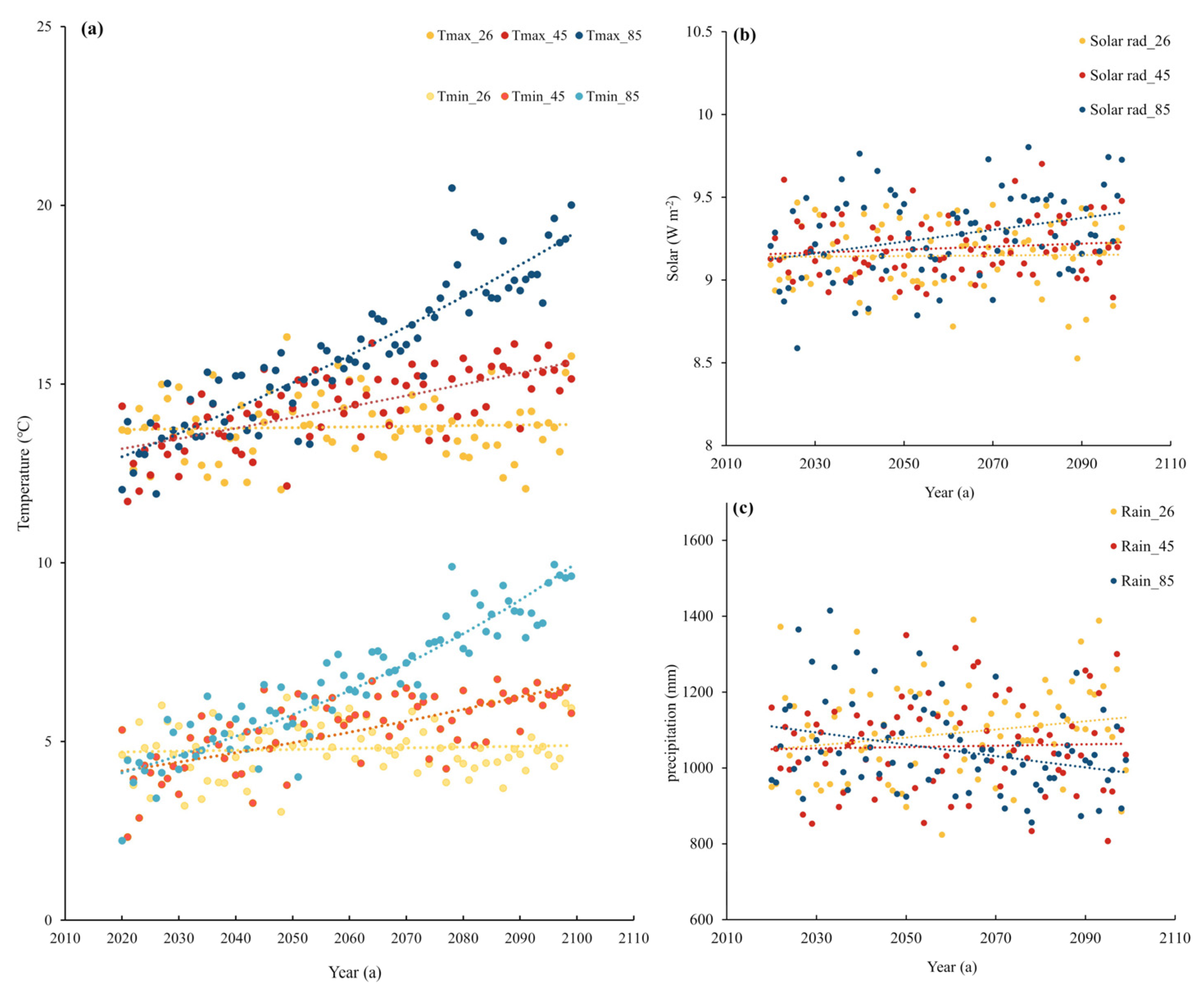
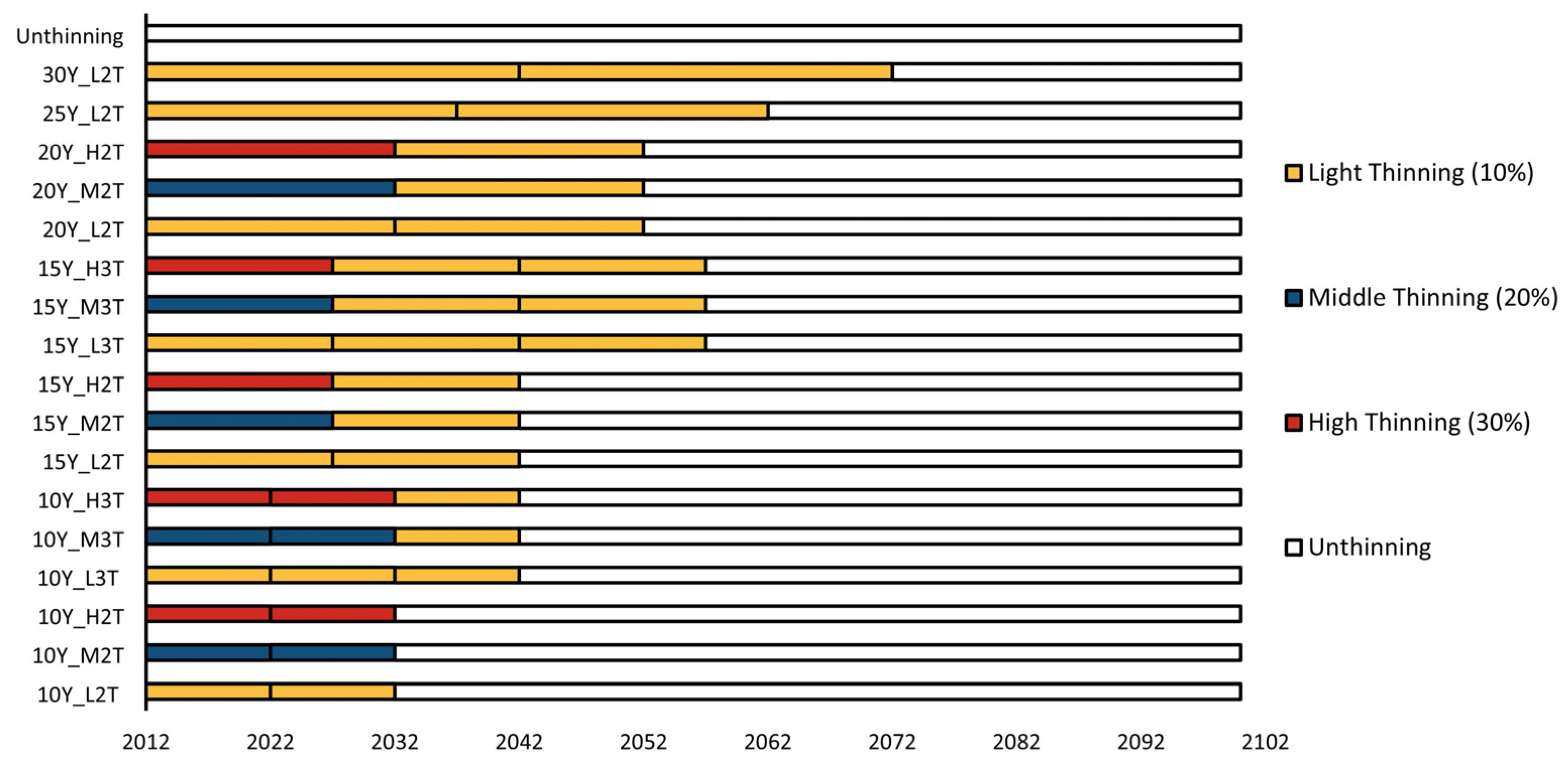
The Coupled Model Intercomparison Project Phase 6 (CMIP6) is a collaborative effort among climate scientists to assess and improve the performance of climate models’ [51]. SSP1-2.6, SSP2-4.5, and SSP5-5.8 are three future projection scenarios in CMIP6, and their primary differences lie in greenhouse gas emissions and climate change predictions. The climate scenarios of SSP1-2.6, SSP2-4.5, and SSP5-5.8 estimate that global warming will be 1.7 °C, 2.0 °C, and 4.4 °C by 2081–2100, respectively. We used the average simulated value of three models—IPSL-CM6A-LR, MPI-ESM1-2-HR, and BCC-CSM2-MR—in the three climate scenarios (Figure A1). To study the synergic effects of climate and thinning on forest growth, we designed 18 thinning regimes for spruce from the Bily Kriz site, including an unthinning control group (Figure 2). Considering that spruce is a coniferous forest and our study plot is an even-aged stand, we only applied the low thinning method to our simulation. We designed the thinning intensity according to the number of trees. The thinning intensity is the proportion of trees cut to the total number of trees in the forest. Considering the ecological characteristics of spruce and its age groups, the stands were thinned at an intensity of 10% (light thinning), 20% (moderate thinning), or 30% (heavy thinning) in the stand stage where they are considered young (age less than 61). In the middle-aged stage, the stand was only lightly thinned. When the stand is near mature (over 90 years of age), thinning operations are no longer carried out. To distinguish the effects of thinning intervals on stand growth, we applied 10-, 15-, 20-, 25-, and 30-year intervals. We added a third thinning operation for shorter intervals (10 or 15 years) based on two thinning operations.

3. Results

3.1. 3-PG Model Calibration and Picea asperata Biomass Simulation

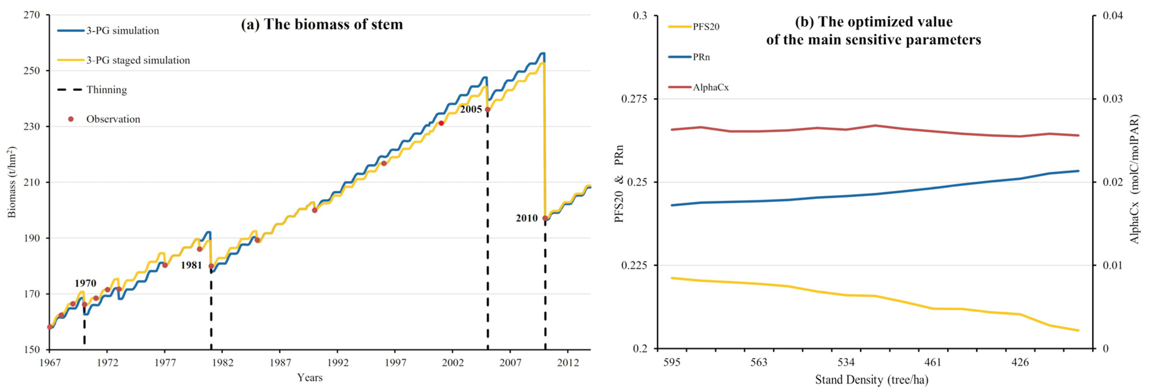
We performed Morris sensitivity analysis using the r3pg package and identified the three most sensitive parameters of the 3-PG model. They are the ratio of leaf biomass to stem productivity when DBH is 20 cm (PFS20), the minimum fraction of NPP to roots (PRn), and the canopy quantum efficiency (AlphaCx), respectively. Parameters related to biomass allocation and photosynthesis are always sensitive to model performance. The model parameterization process and results are similar. Therefore, this section uses the Solling site with the most measured data and the longest temporal range as an example to show the 3-PG calibration results. First, we calibrated the model using all the measured values at the Solling site from 1967 to 2014, as introduced in Section 2.1. There is a deviation between the estimated value (3-PG simulation) and the measured value (Observation) (Figure 3a). From 1967 to 1970, the stand was not thinned, and the estimated value of 3-PG was close to the measured value. But after the first thinning, the model did not properly capture the immediate impact of thinning. This led to a persistent underestimation of stand biomass. After the second thinning in 1981, the model continued to use the original parameters. This can lead to overly optimistic estimates of the stand’s growth potential, resulting in consistently higher estimates. In order to make the estimated value reflect the true situation of the stand as much as possible, we re-optimized the sensitive parameters of the model every time a thinning event occurred. After correcting the parameters in stages, the model simulation results (3-PG staged simulation) were consistent with the observation data. They can meet the data quality requirements of deep learning. Through model simulation, we obtained a total of 3904 augmented data points to support LSTM training. With the decrease in stand density, the optimal values of sensitive parameters in the 3-PG model also change (Figure 3b). As the age of the forest increases and the density of the stand decreases, there is a corresponding increase in the PRn value. In comparison to the initial value, there is a 5.23% increase; PFS20 decreased by 7.09% compared with the initial value, and AlphaCx changed by 2.6% overall from the initial value. The performance of AlphaCx is subject to real-time thinning and exhibits notable fluctuations. A reduction of 100 trees per hectare in stand density resulted in a fluctuation of 13.67% in the parameter value. It is noteworthy that the parameters exhibit a relatively narrow range of variation with respect to their values. Nonetheless, in the 3-PG model, even minor alterations to the aforementioned three critical parameters can significantly impact the model’s trajectory.

3.2. Calibrate and Evaluate the 3PG-MT-LSTM Model

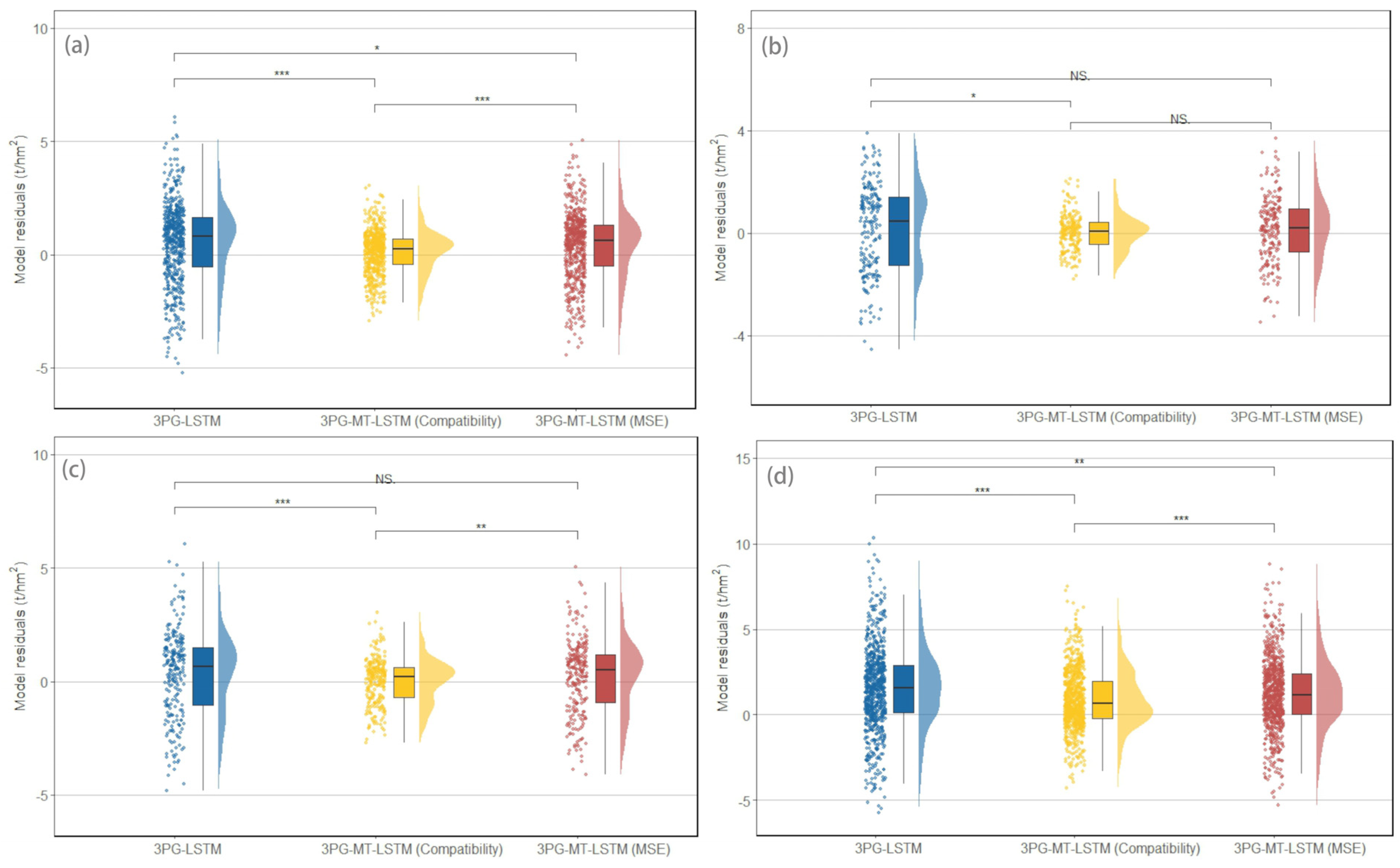
For the present section, we initially employed the residual index to assess the efficacy of 3PG-LSTM, 3PG-MT-LSTM without compatibility rules, and 3PG-MT-LSTM with compatibility rules. Next, we analyzed whether there was a significant difference between the model residuals (Figure 4). Our findings indicate that incoporating biomass compatibility rule into the model can substantially enhance its precision. Simultaneously, the difference between the different models obtained by the Solling site with a large dataset and the joint training of multi-site data is more significant. When the datasets are small, like at the Hyytiala or Bily Kriz sites, the difference in performance between the single-task LSTM models and the multi-task LSTM models is not statistically significant. Following the incorporation of compatibility regulations, in contrast to the solitary-task LSTM model, the performance of the four models was substantially enhanced to differing extents.
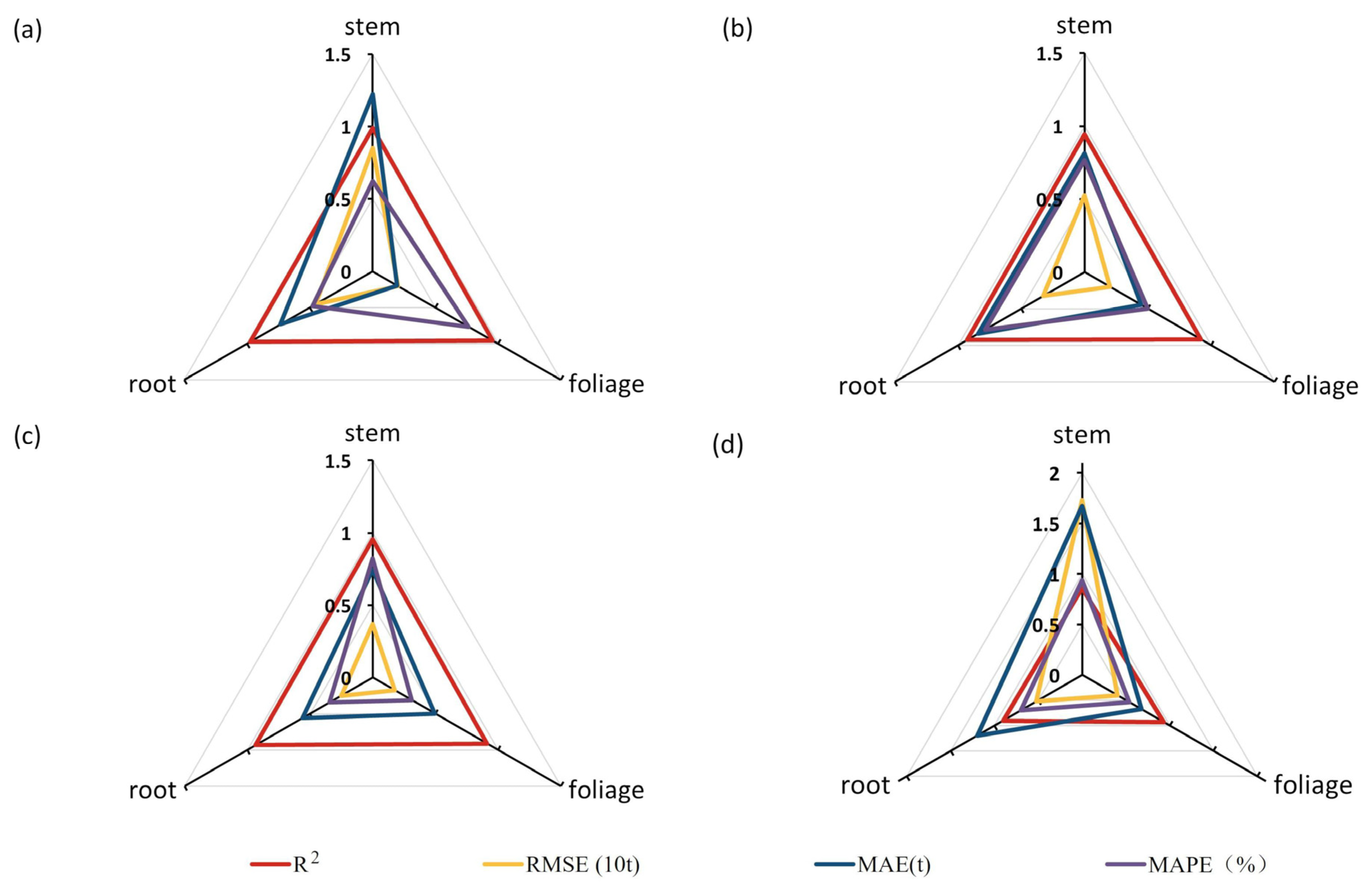
Our assessment of the model was conducted based on the metrics outlined in Section 2.3 (Figure 5). The compatibility rule makes the model more capable of explaining the growth process and variation trend of distinct Norway spruce components (R2 > 0.9). We observed that there is essentially no change in the prediction ability of the model for samples of varying forest ages since MAPE is comparable to the product of MAE and the average value of the data. This demonstrates that the coupling model described in this study performs better and is less susceptible to influence from outside sources. From the ratio of RMSE and MAE (RMSE/MAEsolling_stem = 6.96, RMSE/MAEhyytiala_stem = 6.45, RMSE/MAEbily_stem = 4.95, RMSE/MAEmulti-model_stem = 7.97), it is clear that adding the biomass compatibility rule makes it harder for the model’s forecast process to avoid residual extremes. The model prioritizes minimizing the penalty values of the biomass compatibility loss function and the mean squared error (MSE) loss function. This results in models that sometimes sacrifice the accuracy of individual variables to improve overall model accuracy. Because of the volume and range of the data, the Solling site and multi-site estimation models have larger RMSE and MAE values. The inaccuracy is fairly substantial as a result of the wide variance in the stem biomass.

3.3. Changes in Norway Spruce Biomass under Different Future Climate Scenarios

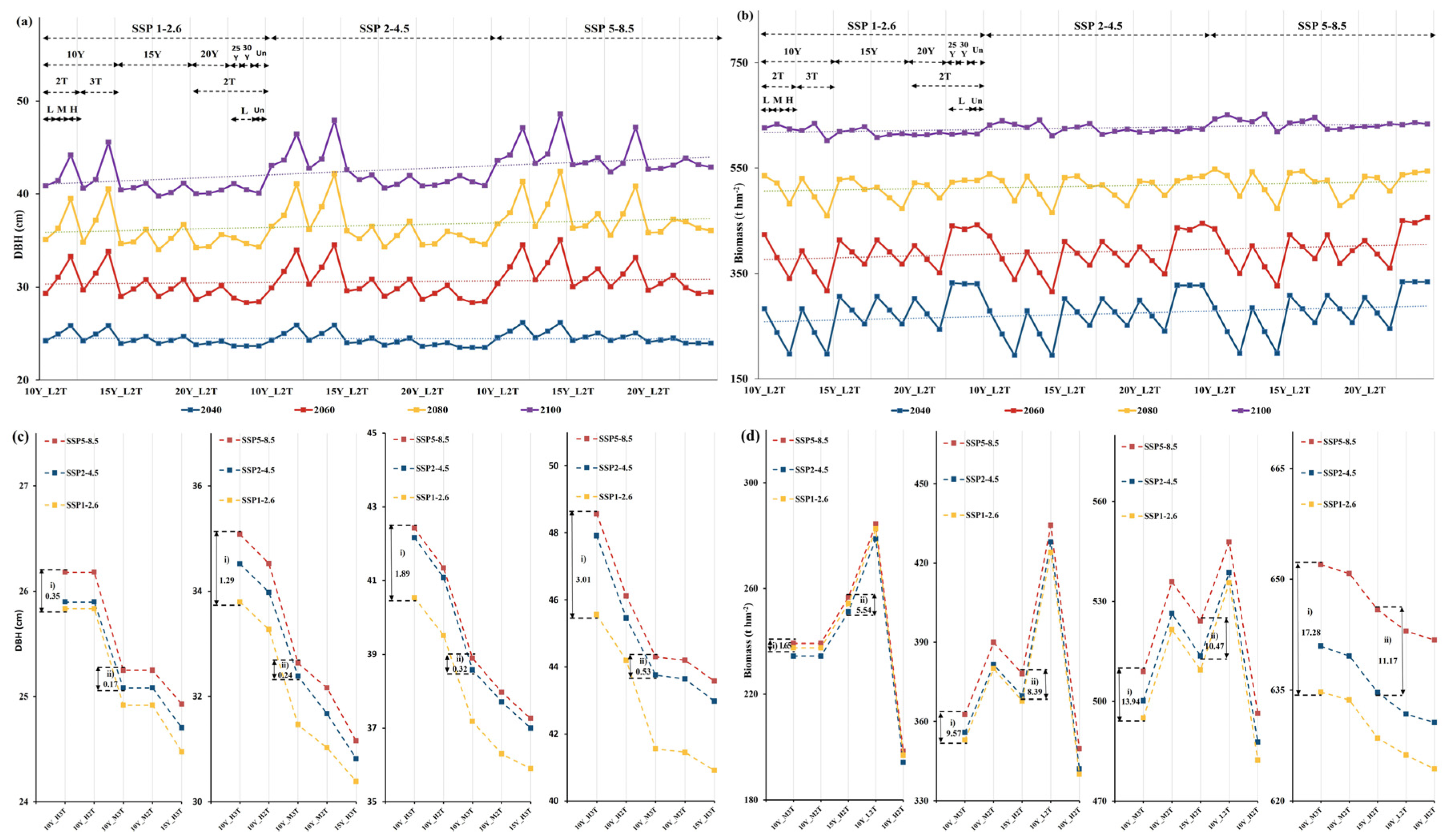
Young, middle-aged, and near-mature forests are the primary types of forests that benefit from thinning as a management strategy [52]. Considering this, in the later stages of the long-term simulation, the spruces in the Hyytiala and Solling sites will reach the mature forest stage. We chose the Bily Kriz site for simulation prediction. We estimated the changing trend of stand biomass and average diameter at breast height using the thinning regimes described and the gathered future climate data in Section 2.4. The ensemble means of three CMIP6 models were utilized to analyze the trend of each meteorological factor (Figure A1). The results indicate that there is a rising trend in the future daily minimum and maximum temperatures, as well as the daily average solar radiation, across all climate scenarios observed at the Bily Kriz site. The results also indicate that, under SSP1-2.6 and SSP2-4.5 scenarios, the precipitation in 2090s increased by 9.79% and 7.02% compared with that in 2010s. On the contrary, under the SSP5-8.5 scenario, the precipitation in 2090s decreased by 12.84% compared with that in 2010s. However, the precipitation in the SSP5-8.5 scenario decreased by 12.84%. The number of frost days had a greater impact on forest productivity. The reduction in the number of frost days persisted because of the steady escalation of the daily minimum temperature within the contexts of the SSP2-4.5 and SSP5-8.5 scenarios. In contrast to the frost days recorded in the 2010s, those observed in the 2090s exhibited a reduction of 40.26% and 69.33% for the respective years. Despite a slight increase in the daily minimum temperature under the SSP1-2.6 scenario, there was no significant alteration in the annual count of frost days. Based on the above climate scenario, we simulated the mean DBH and biomass of Norway spruce at the Bily Kriz site for the 2020–2100 period (Figure 6).
The simulation results indicate that the productivity and DBH growth of spruce were most significant in the SSP5-8.5 scenario, regardless of the combination of thinning intensity and interval, when thinning from below was used (Figure 6a,b). Additionally, with the same thinning intensity and a climate scenario with a higher average temperature, the growth of Norway spruce varied more significantly. We selected the five thinning regimes with the highest biomass and DBH values for spruce in 2100 to verify our views (Figure 6c,d). The figures show the difference in spruce’s response to the same thinning regimes and different climate scenarios at four time nodes in 2040, 2060, 2080, and 2100. Using the 10Y_H3T thinning approach as an example, the difference in DBH between the SSP5-8.5 and SSP1-2.6 scenarios increased from 0.35 cm in 2040 to 3.01 cm in 2100. The difference in biomass increased from 1.65 t hm−2 in 2040 to 17.28 t hm−2 in 2100. The same trend was present among the other thinning regimes (i.e., 10Y_H2T, 10Y_M3T, and other regimes) and climate scenarios. For stand diameter at breast height, with an increase in thinning intensity, the growth rate of stand diameter also increased. However, once the stand age reached 100a (2080), the growth of DBH per unit time began to slow. Furthermore, we discovered that when the thinning frequency was 10 years, the stand diameter was substantially greater than when the cutting frequency was 15 or 20 years. Light thinning at the middle-aged stage of spruce influenced stand diameter, but this effect depended on the thinning intensity at the young stage. For the light- and moderate-thinning plots, the impact on diameter at breast height was not obvious after light thinning in the middle-aged forest stage. However, on highly thinned plots, there was a greater potential for individual tree DBH growth after thinning at the middle-aged forest stage. For stand biomass, the number of Norway spruce trees in the stand fell constantly with increasing thinning severity during the continuous thinning era (before 2060). When compared to the un-thinned instance, the reduced number of trees resulted in lower total biomass. The number of trees was basically stable after the thinning period. When the trees reached the near-mature forest stage in 2080, the productivity of the 10Y_LT and 10Y_MT thinning forests were higher than that of the non-thinned stands. In 2100, The 10-year-cut and 15-year-cut stands’ productivity was at a relatively high level, and the trees still had great growth potential. When Norway spruce is young, moderate-to-heavy thinning of the stand every 10 years makes it easier to produce large-diameter timber. Thinning at extended time intervals (more than 20 years) not only inhibits the growth of single-tree diameter at breast height but also limits the increase in total biomass.

4. Discussion

4.1. Estimation Accuracy and Interpretability of the Hybrid Model

The 3-PG model is designed to simulate key processes in the growth of forest stands. The model necessitates numerous parameters, and acquiring their values through direct observation is a challenging task [53]. Utilizing the LSTM approach driven by data, it is possible to effectively extract the spatio-temporal features of stand growth and their associations with climate, geography, and anthropogenic factors, based on historical data [54,55]. The process of training deep learning models typically necessitates a substantial amount of data. This study utilized the optimized 3-PG model to address the challenge of acquiring biomass data by boosting the available observation data. A substantial quantity of superior-grade data needs to be acquired to bolster the training of the LSTM model. The present study incorporates LSTM as a shared layer, multi-task learning, and biomass compatibility rules. The model adheres to the fundamental principle of mass conservation. Improvements in estimation accuracy, reliability, and generalization ability were also observed. The 3PG-MT-LSTM model more accurately captures the impact of thinning and climate change on stand biomass. The reasonable use of models for prediction and estimation can reduce uncertainty in forest management.
The density of tree stands is a crucial factor in determining the level of competition for resources among trees, ultimately impacting their growth [56,57]. The Norway spruce at the Solling site transitions from near-mature forest to mature forest. Thinning alters the structure of the canopy, allowing more light to reach the understory, which promotes forest growth. However, according to the studies described in Section 3.1, the age of the forest is a constraint that causes the photosynthetic efficacy of trees (or AlphaCx) to fluctuate and decline. The decrease in the PFS20 parameter value can also reflect the change in forest photosynthetic efficiency. After thinning, the leaf area index decreases, the gap increases, and each tree is allocated more appropriate growing space. The light resource is no longer the main object of tree competition. Whilst there was a gradual increase in leaf biomass, there was a decrease in the proportion of biomass that trees allocated to leaves. This discovery is in line with the research conducted by Deng et al. [58] and Chen et al. [59]. On the other hand, soil resources are finite. As forest grows, there is a concomitant decrease in soil fertility for a given plot. At this time, there is a tendency for forest stands to allocate a greater amount of carbon towards their root system, resulting in an increase in the PRn parameter. This phenomenon has the potential to enhance the competitive advantage of vegetation in acquiring soil resources. Competition for biomass allocation among stand organs is considered to be an adaptive feature of forests [60]. Similar findings were reported by Wang et al. [61] and Subedi et al. [62] in their respective investigations of the effects of thinning on tree biomass distribution.
It is challenging to adequately depict forest tree growth using a “white box” model because it is a complex process. For instance, the spatiotemporal dependence of vegetation and physiological and ecological characteristics needs to be considered in the prediction process. The LSTM regulates the flow and output of information by means of its distinctive gating mechanism. In contrast to Artificial Neural Networks and Recurrent Neural Networks, LSTM exhibits superior capacity in acquiring long-term dependencies within a sequence [63]. The temporal correlation between climate-induced effects on forests remains unclear. This is difficult to explain and quantify using known mechanisms [64,65]. Because of its gating mechanism, LSTM is better suited to processing and predicting a long-time series with relatively large intervals and delays [66,67]. LSTM can accurately capture the effect of events on forest biomass, whether it be forest thinning with extended gap intervals or climatic change with lag effects. While LSTM models can achieve high levels of accuracy during training, it is important to remain cautious of their inherent uncertainty. The constraints of physical processes must also be considered while maximizing knowledge learning from data. The 3-PG model exhibited more accuracy in simulating the allometric growth of the tree. The output of the process model was employed as the training sample for deep learning for this paper, and underlying physical law restrictions were introduced in the training process. The aforementioned approach not only satisfies the data prerequisites of Long Short-Term Memory (LSTM) and enhances the precision of the model but also upholds a degree of conformity with the principles governing plant growth. Through multi-task learning and penalty terms in loss function, the 3PG-MT-LSTM model integrates biomass compatibility rules. In forest ecosystems, the biomass compatibility rule is a rare and strong physical limitation. The principles of mass conservation-based compatibility rules are universally applicable to trees of all species, regardless of the age of the forest or its geographical location. During our research, we also considered models of volume compatibility (i.e., biomass = plant volume * plant density). However, after discussion, we discovered that the density of wood will alter slightly with the expansion of forest age, even for the same tree species. Additionally, obtaining the volume also presents challenges. This could cause the model to contain more mistakes and uncertainties. Because of this, for this study, we ultimately decided to solely employ the biomass compatibility constraint as the model’s additional penalty. In deep learning algorithms, this reduces the build-up of unjustified errors. The accuracy of the 3PG-MT-LSTM model remains unaffected by variations in forest age or external environmental factors, irrespective of whether the model is trained on a single site or multiple sites. The integration of process modeling, and deep learning techniques enhances the predictive capabilities of the model in predicting future changes, thereby introducing a novel avenue for precision forestry research.

4.2. Synergistic Effects of Thinning and Climate on Forest Growth

Examining the relationship between tree growth and environmental and management practices is a crucial aspect of the advancement of precision forestry. In the young forest stage, stand density is generally higher. Thinning reduces competition among trees for nutrient space and resource constraints on tree growth. Based on the 3PG-MT-LSTM model proposed in this paper, we performed long-term predictions of Norway spruce biomass at the Bily Kriz site. The results showed that, when using the identical thinning strategy, SSP5-8.5’s simulation of Norway spruce had the highest overall biomass and single-tree diameter. After combining the differences between different climate scenarios in Section 3.3, we can conclude that solar radiation and temperature are the most important driving variables for Norway spruce growth without considering the impact of extreme climates. This agrees with conclusions from earlier studies examining the environmental factors that influence spruce growth [68,69,70]. The observed variations in DBH and biomass across different scenarios indicate that the beneficial impact of forest management is particularly pronounced in warmer climates. The differences observed in SSP5-8.5 compared to other scenarios have evidenced that the Norway spruce species exhibits favorable ecological adaptability and thrives in areas with abundant sunlight and moderate humidity levels. The Norway spruce species can tolerate a variety of environmental conditions but prefers a climate with moderate humidity and lots of sunlight [71]. Temperature and solar radiation will exponentially increase after the 2070s, according to the SSP5-8.5 climate change scenario (Figure A1). The amount of precipitation exhibited a further decrease. As a result, in the SSP5-8.5 scenario, Norway spruce growth continued to increase. But compared to other situations, the growth rate was lower.
Different thinning intensities and intervals had a substantial impact on stand growth, in addition to climate change. The regimes taken during the young-aged forest stage for thinning played a decisive role in the growth of the stand’s average diameter at breast height. For even-aged spruce forests, we used low thinning to reduce stand density and intra-stand competition. Under the low-thinning method, the heavy thinning of stands in young forests is conducive to the production of large-diameter timber. On this basis, further light thinning of stands in the middle-aged forest stage can increase the growth potential of stand diameter at breast height. Over time, the growth rate of a single tree in the light-to-moderate thinning stand slowed down significantly (at the same time interval, the average increase in diameter at breast height decreased). This is due to the limitations of light resources and soil resources [72]. Managers can improve ventilation and light conditions in the forest at this time by pruning branches and increasing forest gaps. In the thinning stage, there was an inverse relationship between thinning intensity and stand biomass. The higher the thinning intensity, the smaller the stand number and remaining biomass. This is consistent with the findings of Simon and Ameztegui [73]. After thinning, the stand entered a rapid growth period. In Section 3.3, we found that the growth rate of biomass in moderate- and heavy-thinning forests is much higher than that of light-thinning forests. In 2100, the biomass of moderate-thinning stands was the highest compared with other thinning regimes. This is a consequence of the regulation of multiple conditions, such as the total number of trees, soil resources, and competition within the forest. Rimal et al. examined the effects of different thinning intensities and intervals on the biomass growth of a 75-year-old Norway spruce stand [13]. They found that light thinning applied at longer intervals (greater than 25 years) resulted in higher stand biomass. However, according to our research, conducting moderate-to-heavy thinning 1–2 times during the young-aged Norway spruce forest stage and light thinning 0–2 times during the middle-aged forest stage are more favorable for biomass accumulation. The 10Y_H2T thinning regime can better balance the relationship between DBH and production. We attributed the differences in Rimal et al.‘s results to the difference in the ages of the subjects. Specifically, our study was conducted on a 34-year-old forest stand, whereas Rimal et al. conducted their research on a 75-year-old one. Consequently, variations exist in the choice of thinning techniques and the resultant findings.
In the context of forest stand management, it may be advisable to conduct heavy thinning during the early stages of stand development in instances where there is a high demand for large-diameter timber. This approach is particularly relevant for operators in this field. To enhance the stand’s overall productivity within a limited timeframe, opting for light thinning as a stand management strategy is advisable. To maximize the stand’s long-term carbon sink capacity, we recommend implementing periodic moderate thinning with intervals of 10 to 15 years during the young-aged forest stage. Using the 3PG-MT-LSTM model has the potential to aid forest managers in promptly revising stand growth information. Before thinning, operators can formulate suitable thinning measures based on the results of model simulations. This can provide a direction to help them achieve a balance between producing large-diameter timber and economic benefits while taking forest carbon storage into account. After thinning, the model can be used to continuously monitor the growth of forest stands. By evaluating the real-time impact of management measures on the value of forest carbon sinks, operators can promote the development of sustainable forest management.

4.3. Limitations of Modeling Methods

The 3-PG model provides a larger training sample for deep learning algorithms. At the same time, the cost of data collection is reduced. However, limited by the output of the 3-PG model, we can only constrain the compatibility rules among stem, leaf, root, aboveground biomass, and total biomass. The biomass of bark and branches cannot be estimated. Due to constraints in data acquisition during the variable selection process, variables such as soil fertility were not included. Although the 3-PG sub-model has the capability to simulate alterations in soil fertility. To mitigate the potential for heightened ambiguity within the model, we refrained from incorporating its simulated value as a feature variable. Furthermore, we lack thinning regime designs for different thinning methods. Our model currently only provides forest growth estimates for a single thinning method. In the future, we hope to obtain more relevant data support, combined with feature coding technology, to design a more complete thinning experiment. This provides a reliable technical means of clarifying the long-term impacts of thinning on forests.
For the 3PG-MT-LSTM model, in addition to increasing the type and amount of data, the coupling mechanism is also an important avenue for improvement. Despite the fact that the interpretability of the hybrid model has improved, it fundamentally remains a model driven by data. The model exhibits a high degree of precision in its response to alterations in both climatic and human management factors. However, the challenge lies in accurately measuring the individual impact of each variable on the simulation outcomes. During the process of training a model, there is a relatively high demand for professional expertise and hardware capabilities, resulting in a relatively high computational cost. Researchers will be able to build genuine data–mechanism hybrid driving models in the future using methods such as mechanism model parameter optimization, model sub-module proxy, and model system error correction. This could further improve the robustness of forestry model and provides technical support for forestry accurate management.

5. Conclusions

Data gaps are a common problem in forestry modeling. In this paper, combined with the existing data parameterizing the 3-PG model, the stand diameter and biomass data were successfully filled using the monthly scale simulation results. The LSTM is trained based on the augmented data, and the 3PG-MT-LSTM model is constructed by adding MTL and compatibility rules. In contrast to the conventional LSTM architecture, the coupling model demonstrates enhanced precision in biomass estimation following thinning operations while also circumventing the accumulation of errors across individual components. There is no significant difference in the applicability of the model when it is applied to spruce forest stands in different regions and forest ages, and the generalization ability has improved. Utilizing the hybrid model, the present study showcases the impact of diverse thinning techniques on the growth of Norway spruce trees situated at the Bily Kriz location in light of anticipated climate change scenarios. According to our analysis, the periodic light-to-moderate thinning of Norway spruce stands at intervals of 10 to 15 years had a favorable impact on the accumulation of biomass over an extended period.
The heavy thinning technique is deemed more appropriate to produce timber with large diameters. Additionally, thinning management during the young-aged stages of forest growth is imperative for any production objective. The decision to implement additional management practices during the middle-aged stage of forest growth can be appropriately modified based on the current condition of the stand. The application of a hybrid model can help managers balance large-diameter timber production with economic benefits. The carbon sink value of a stand is determined through comprehensive research to provide scientific guidance for sustainable forest development. In conclusion, the in-depth application of deep learning presents an opportunity for the field of forestry management, but it also poses new challenges for forest managers.

Author Contributions

Conceptualization, J.Q. and X.S.; methodology, J.Q.; validation, J.Q., X.S. and M.M.; formal analysis, J.Q.; data curation, Y.Z.; writing—original draft preparation, J.Q.; writing—review and editing, X.S. and B.W.; visualization, J.Q., M.M. and X.S. All authors have read and agreed to the published version of the manuscript.

Funding

This research was funded by National Natural Science Foundation of China, grant number 32101516.

Institutional Review Board Statement

Not applicable for studies not involving humans or animals.

Informed Consent Statement

Not applicable for studies not involving humans.

Data Availability Statement

The data that support the findings of this study are openly available in the “PROFOUND database” (https://doi.org/10.5880/PIK.2020.006, accessed on 12 December 2022) and “The Coupled Model Intercomparison Project Phase 6” (https://esgf-node.llnl.gov/projects/cmip6/, accessed on 14 February 2023).

Acknowledgments

We thank the makers of the PROFOUND database for providing free access to their data. We acknowledge the World Climate Research Program’s Working Group on Coupled Modeling, which is responsible for CMIP6, and thank the climate modeling groups for producing and making available their model outputs. We also thank the anonymous reviewers for their valuable suggestions.

Conflicts of Interest

The authors declare no conflict of interest.

Appendix A

Figure A1. Change trends of annual average maximum and minimum temperature (a), annual average solar radiation (b), and annual total precipitation (c) under SSP1-2.6, SSP2-4.5, and SSP5-8.5 scenarios. The values shown here are from the same source as the future meteorological factors in the text. They are taken from the ensemble averages of three climate models: IPSL-CM6A-LR, MPI-ESM1-2-HR, and BCC-CSM2-MR.
Forests 14 01482 g0a1

References

  1. Kramer, P.J. Carbon Dioxide Concentration, Photosynthesis, and Dry Matter Production. BioScience 1981, 31, 29–33. [Google Scholar] [CrossRef]
  2. Reichstein, M.; Carvalhais, N. Aspects of Forest Biomass in the Earth System: Its Role and Major Unknowns. Surv. Geophys. 2019, 40, 693–707. [Google Scholar] [CrossRef] [Green Version]
  3. Yadav, V.S.; Yadav, S.S.; Gupta, S.R.; Meena, R.S.; Lal, R.; Sheoran, N.S.; Jhariya, M.K. Carbon Sequestration Potential and CO2 Fluxes in a Tropical Forest Ecosystem. Ecol. Eng. 2022, 176, 106541. [Google Scholar] [CrossRef]
  4. Hansen, W.D.; Schwartz, N.B.; Williams, A.P.; Albrich, K.; Kueppers, L.M.; Rammig, A.; Reyer, C.P.O.; Staver, A.C.; Seidl, R. Global Forests Are Influenced by the Legacies of Past Inter-Annual Temperature Variability. Environ. Res. Ecol. 2022, 1, 011001. [Google Scholar] [CrossRef]
  5. Augusto, L.; Boča, A. Tree Functional Traits, Forest Biomass, and Tree Species Diversity Interact with Site Properties to Drive Forest Soil Carbon. Nat. Commun. 2022, 13, 1097. [Google Scholar] [CrossRef] [PubMed]
  6. Erdozain, M.; Bonet, J.A.; Martínez de Aragón, J.; de-Miguel, S. Forest Thinning and Climate Interactions Driving Early-Stage Regeneration Dynamics of Maritime Pine in Mediterranean Areas. For. Ecol. Manag. 2023, 539, 121036. [Google Scholar] [CrossRef]
  7. Yu, J.; Zhang, X.; Xu, C.; Hao, M.; Choe, C.; He, H. Thinning Can Increase Shrub Diversity and Decrease Herb Diversity by Regulating Light and Soil Environments. Front. Plant Sci. 2022, 13, 948648. [Google Scholar] [CrossRef]
  8. Zhang, X.; Guan, D.; Li, W.; Sun, D.; Jin, C.; Yuan, F.; Wang, A.; Wu, J. The Effects of Forest Thinning on Soil Carbon Stocks and Dynamics: A Meta-Analysis. For. Ecol. Manag. 2018, 429, 36–43. [Google Scholar] [CrossRef]
  9. D’Amato, A.W.; Bradford, J.B.; Fraver, S.; Palik, B.J. Effects of Thinning on Drought Vulnerability and Climate Response in North Temperate Forest Ecosystems. Ecol. Appl. 2013, 23, 1735–1742. [Google Scholar] [CrossRef] [Green Version]
  10. Gong, C.; Tan, Q.; Liu, G.; Xu, M. Forest Thinning Increases Soil Carbon Stocks in China. For. Ecol. Manag. 2021, 482, 118812. [Google Scholar] [CrossRef]
  11. Olajuyigbe, S.; Tobin, B.; Saunders, M.; Nieuwenhuis, M. Forest Thinning and Soil Respiration in a Sitka Spruce Forest in Ireland. Agric. For. Meteorol. 2012, 157, 86–95. [Google Scholar] [CrossRef]
  12. Melikov, C.H.; Bukoski, J.J.; Cook-Patton, S.C.; Ban, H.; Chen, J.L.; Potts, M.D. Quantifying the Effect Size of Management Actions on Aboveground Carbon Stocks in Forest Plantations. Curr. For. Rep. 2023, 9, 131–148. [Google Scholar] [CrossRef] [PubMed]
  13. Rimal, S.; Djahangard, M.; Yousefpour, R. Forest Management under Climate Change: A Decision Analysis of Thinning Interventions for Water Services and Biomass in a Norway Spruce Stand in South Germany. Land 2022, 11, 446. [Google Scholar] [CrossRef]
  14. Heimann, M.; Reichstein, M. Terrestrial Ecosystem Carbon Dynamics and Climate Feedbacks. Nature 2008, 451, 289–292. [Google Scholar] [CrossRef] [PubMed] [Green Version]
  15. Higgins, S.I.; Conradi, T.; Muhoko, E. Shifts in Vegetation Activity of Terrestrial Ecosystems Attributable to Climate Trends. Nat. Geosci. 2023, 16, 147–153. [Google Scholar] [CrossRef]
  16. Beer, C.; Reichstein, M.; Tomelleri, E.; Ciais, P.; Jung, M.; Carvalhais, N.; Rödenbeck, C.; Arain, M.A.; Baldocchi, D.; Bonan, G.B.; et al. Terrestrial Gross Carbon Dioxide Uptake: Global Distribution and Covariation with Climate. Science 2010, 329, 834–838. [Google Scholar] [CrossRef] [Green Version]
  17. Medlyn, B.E.; Pepper, D.A.; O’Grady, A.P.; Keith, H. Linking Leaf and Tree Water Use with an Individual-Tree Model. Tree Physiol. 2007, 27, 1687–1699. [Google Scholar] [CrossRef] [Green Version]
  18. Sturtevant, B.R. Forest Processes from Stands to Landscapes: Exploring Model Forecast Uncertainties Using Cross-Scale Model Comparison. Can. J. For. Res. 2010, 40, 2345–2359. [Google Scholar] [CrossRef] [Green Version]
  19. Landsberg, J.J.; Waring, R.H. A Generalised Model of Forest Productivity Using Simplified Concepts of Radiation-Use Efficiency, Carbon Balance and Partitioning. For. Ecol. Manag. 1997, 95, 209–228. [Google Scholar] [CrossRef]
  20. Restrepo, H.I.; Montes, C.R.; Bullock, B.P.; Mei, B. The Effect of Climate Variability Factors on Potential Net Primary Productivity Uncertainty: An Analysis with a Stochastic Spatial 3-PG Model. Agric. For. Meteorol. 2022, 315, 108812. [Google Scholar] [CrossRef]
  21. Running, S.W.; Coughlan, J.C. A General Model of Forest Ecosystem Processes for Regional Applications I. Hydrologic Balance, Canopy Gas Exchange and Primary Production Processes. Ecol. Model. 1988, 42, 125–154. [Google Scholar] [CrossRef]
  22. Yan, M.; Mao, F.; Du, H.; Li, X.; Chen, Q.; Ni, C.; Huang, Z.; Xu, Y.; Gong, Y.; Guo, K.; et al. Spatiotemporal Dynamic of Subtropical Forest Carbon Storage and Its Resistance and Resilience to Drought in China. Front. Plant Sci. 2023, 14, 1067552. [Google Scholar] [CrossRef] [PubMed]
  23. Dang, A.T.N.; Nandy, S.; Srinet, R.; Luong, N.V.; Ghosh, S.; Senthil Kumar, A. Forest Aboveground Biomass Estimation Using Machine Learning Regression Algorithm in Yok Don National Park, Vietnam. Ecol. Inform. 2019, 50, 24–32. [Google Scholar] [CrossRef]
  24. Huy, B.; Truong, N.Q.; Khiem, N.Q.; Poudel, K.P.; Temesgen, H. Deep Learning Models for Improved Reliability of Tree Aboveground Biomass Prediction in the Tropical Evergreen Broadleaf Forests. For. Ecol. Manag. 2022, 508, 120031. [Google Scholar] [CrossRef]
  25. Kraft, B.; Jung, M.; Körner, M.; Requena Mesa, C.; Cortés, J.; Reichstein, M. Identifying Dynamic Memory Effects on Vegetation State Using Recurrent Neural Networks. Front. Big Data 2019, 2, 31. [Google Scholar] [CrossRef] [Green Version]
  26. De Oliveira Neto, R.R.; Leite, H.G.; Gleriani, J.M.; Strimbu, B.M. Estimation of Eucalyptus Productivity Using Efficient Artificial Neural Network. Eur. J. For. Res. 2022, 141, 129–151. [Google Scholar] [CrossRef]
  27. Xu, Q.; Lei, X.; Zhang, H. A Novel Method for Approaching the Compatibility of Tree Biomass Estimation by Multi-Task Neural Networks. For. Ecol. Manag. 2022, 508, 120011. [Google Scholar] [CrossRef]
  28. Gu, Y.; Li, B.; Meng, Q. Hybrid Interpretable Predictive Machine Learning Model for Air Pollution Prediction. Neurocomputing 2022, 468, 123–136. [Google Scholar] [CrossRef]
  29. Narayanan, H.; Cruz Bournazou, M.N.; Guillén Gosálbez, G.; Butté, A. Functional-Hybrid Modeling through Automated Adaptive Symbolic Regression for Interpretable Mathematical Expressions. Chem. Eng. J. 2022, 430, 133032. [Google Scholar] [CrossRef]
  30. Perry, G.L.W.; Seidl, R.; Bellvé, A.M.; Rammer, W. An Outlook for Deep Learning in Ecosystem Science. Ecosystems 2022, 25, 1700–1718. [Google Scholar] [CrossRef]
  31. Irrgang, C.; Boers, N.; Sonnewald, M.; Barnes, E.A.; Kadow, C.; Staneva, J.; Saynisch-Wagner, J. Towards Neural Earth System Modelling by Integrating Artificial Intelligence in Earth System Science. Nat. Mach. Intell. 2021, 3, 667–674. [Google Scholar] [CrossRef]
  32. Reichstein, M.; Camps-Valls, G.; Stevens, B.; Jung, M.; Denzler, J.; Carvalhais, N. Prabhat Deep Learning and Process Understanding for Data-Driven Earth System Science. Nature 2019, 566, 195–204. [Google Scholar] [CrossRef] [PubMed]
  33. Konapala, G.; Kao, S.-C.; Painter, S.L.; Lu, D. Machine Learning Assisted Hybrid Models Can Improve Streamflow Simulation in Diverse Catchments across the Conterminous US. Environ. Res. Lett. 2020, 15, 104022. [Google Scholar] [CrossRef]
  34. Xu, T.; Longyang, Q.; Tyson, C.; Zeng, R.; Neilson, B.T. Hybrid Physically Based and Deep Learning Modeling of a Snow Dominated, Mountainous, Karst Watershed. Water Resour. Res. 2022, 58, e2021WR030993. [Google Scholar] [CrossRef]
  35. Jiang, S.; Zheng, Y.; Solomatine, D. Improving AI System Awareness of Geoscience Knowledge: Symbiotic Integration of Physical Approaches and Deep Learning. Geophys. Res. Lett. 2020, 47, e2020GL088229. [Google Scholar] [CrossRef]
  36. Li, M.; Yang, Y.; He, Z.; Guo, X.; Zhang, R.; Huang, B. A Wind Speed Forecasting Model Based on Multi-Objective Algorithm and Interpretability Learning. Energy 2023, 269, 126778. [Google Scholar] [CrossRef]
  37. Wang, T.; Lin, Q. Hybrid Predictive Models: When an Interpretable Model Collaborates with a Black-Box Model. J. Mach. Learn. Res. 2021, 22, 6085–6122. [Google Scholar]
  38. Pradhan, K.; Ettinger, A.K.; Case, M.J.; Hille Ris Lambers, J. Applying Climate Change Refugia to Forest Management and Old-Growth Restoration. Glob. Chang. Biol. 2023, 29, 3692–3706. [Google Scholar] [CrossRef]
  39. Reyer, C.P.; Silveyra Gonzalez, R.; Dolos, K.; Hartig, F.; Hauf, Y.; Noack, M.; Lasch-Born, P.; Rötzer, T.; Pretzsch, H.; Meesenburg, H.; et al. The PROFOUND Database for Evaluating Vegetation Models and Simulating Climate Impacts on European Forests. Earth Syst. Sci. Data 2020, 12, 1295–1320. [Google Scholar] [CrossRef]
  40. Sands, P.J.; Landsberg, J.J. Parameterisation of 3-PG for Plantation Grown Eucalyptus Globulus. For. Ecol. Manag. 2002, 163, 273–292. [Google Scholar] [CrossRef]
  41. Song, X.; Song, Y. Introducing 3-PG2Py, an Open-Source Forest Growth Model in Python. Environ. Model. Softw. 2022, 150, 105358. [Google Scholar] [CrossRef]
  42. Wallach, D.; Makowski, D.; Jones, J.W.; Brun, F. Chapter 3—The R Programming Language and Software. In Working with Dynamic Crop Models, 2nd ed.; Wallach, D., Makowski, D., Jones, J.W., Brun, F., Eds.; Academic Press: San Diego, CA, USA, 2014; pp. 71–117. ISBN 978-0-12-397008-4. [Google Scholar]
  43. Trotsiuk, V.; Hartig, F.; Forrester, D.I. R3PG—An r Package for Simulating Forest Growth Using the 3-PG Process-Based Model. Methods Ecol. Evol. 2020, 11, 1470–1475. [Google Scholar] [CrossRef]
  44. Morris, M.D. Factorial Sampling Plans for Preliminary Computational Experiments. Technometrics 1991, 33, 161–174. [Google Scholar] [CrossRef]
  45. Caruana, R. Multitask Learning. Mach. Learn. 1997, 28, 41–75. [Google Scholar] [CrossRef]
  46. Wang, Y.; Zhang, D.; Wulamu, A. A Multitask Learning Model with Multiperspective Attention and Its Application in Recommendation. Comput. Intell. Neurosci. 2021, 2021, 8550270. [Google Scholar] [CrossRef] [PubMed]
  47. Qi, Y.; Li, Q.; Karimian, H.; Liu, D. A Hybrid Model for Spatiotemporal Forecasting of PM2.5 Based on Graph Convolutional Neural Network and Long Short-Term Memory. Sci. Total Environ. 2019, 664, 1–10. [Google Scholar] [CrossRef]
  48. Wang, S.; Ren, Y.; Xia, B.; Liu, K.; Li, H. Prediction of Atmospheric Pollutants in Urban Environment Based on Coupled Deep Learning Model and Sensitivity Analysis. Chemosphere 2023, 331, 138830. [Google Scholar] [CrossRef]
  49. Seltzer, M.L.; Droppo, J. Multi-Task Learning in Deep Neural Networks for Improved Phoneme Recognition. In Proceedings of the 2013 IEEE International Conference on Acoustics, Speech and Signal Processing, Vancouver, BC, Canada, 26–31 May 2013; pp. 6965–6969. [Google Scholar]
  50. Zhang, Y.; Yang, Q. An Overview of Multi-Task Learning. Natl. Sci. Rev. 2018, 5, 30–43. [Google Scholar] [CrossRef] [Green Version]
  51. Carvalho, D.; Rafael, S.; Monteiro, A.; Rodrigues, V.; Lopes, M.; Rocha, A. How Well Have CMIP3, CMIP5 and CMIP6 Future Climate Projections Portrayed the Recently Observed Warming. Sci. Rep. 2022, 12, 11983. [Google Scholar] [CrossRef]
  52. Wang, Y.; Wei, X.; del Campo, A.D.; Winkler, R.; Wu, J.; Li, Q.; Liu, W. Juvenile Thinning Can Effectively Mitigate the Effects of Drought on Tree Growth and Water Consumption in a Young Pinus Contorta Stand in the Interior of British Columbia, Canada. For. Ecol. Manag. 2019, 454, 117667. [Google Scholar] [CrossRef]
  53. Zhou, F.; Chai, F.; Huang, D.; Xue, H.; Chen, J.; Xiu, P.; Xuan, J.; Li, J.; Zeng, D.; Ni, X.; et al. Investigation of Hypoxia off the Changjiang Estuary Using a Coupled Model of ROMS-CoSiNE. Prog. Oceanogr. 2017, 159, 237–254. [Google Scholar] [CrossRef]
  54. Willard, J.; Jia, X.; Xu, S.; Steinbach, M.; Kumar, V. Integrating Scientific Knowledge with Machine Learning for Engineering and Environmental Systems. ACM Comput. Surv. 2022, 55, 66. [Google Scholar] [CrossRef]
  55. Zhang, Q.; Wang, R.; Qi, Y.; Wen, F. A Watershed Water Quality Prediction Model Based on Attention Mechanism and Bi-LSTM. Environ. Sci. Pollut. Res. 2022, 29, 75664–75680. [Google Scholar] [CrossRef]
  56. Geng, Y.; Yue, Q.; Zhang, C.; Zhao, X.; von Gadow, K. Dynamics and Drivers of Aboveground Biomass Accumulation during Recovery from Selective Harvesting in an Uneven-Aged Forest. Eur. J. For. Res. 2021, 140, 1163–1178. [Google Scholar] [CrossRef]
  57. Zhou, H.; Meng, S.; Liu, Q. Long-Term Response of Living Forest Biomass to Extensive Logging in Subtropical China. J. For. Res. 2019, 30, 1679–1687. [Google Scholar] [CrossRef]
  58. Deng, C.; Ma, F.; Xu, X.; Zhu, B.; Tao, J.; Li, Q. Allocation Patterns and Temporal Dynamics of Chinese Fir Biomass in Hunan Province, China. Forests 2023, 14, 286. [Google Scholar] [CrossRef]
  59. Chen, R.; Ran, J.; Hu, W.; Dong, L.; Ji, M.; Jia, X.; Lu, J.; Gong, H.; Aqeel, M.; Yao, S.; et al. Effects of Biotic and Abiotic Factors on Forest Biomass Fractions. Natl. Sci. Rev. 2021, 8, nwab025. [Google Scholar] [CrossRef]
  60. Zhang, W.-P.; Jia, X.; Morris, E.C.; Bai, Y.-Y.; Wang, G.-X. Stem, Branch and Leaf Biomass-Density Relationships in Forest Communities. Ecol. Res. 2012, 27, 819–825. [Google Scholar] [CrossRef]
  61. Wang, Z.C.; Li, Y.X.; Meng, Y.B.; Wang, C. Effect of Tending and Thinning on Spatial and Carbon Distribution Patterns of Natural Mixed Broadlesf-Conifer Secondary Forest in Xiaoxing’an Mountains, Pr China. Appl. Ecol. Environ. Res. 2021, 19, 4751–4764. [Google Scholar] [CrossRef]
  62. Subedi, S.; Kane, M.; Zhao, D.; Borders, B.; Greene, D. Cultural Intensity and Planting Density Effects on Aboveground Biomass of 12-Year-Old Loblolly Pine Trees in the Upper Coastal Plain and Piedmont of the Southeastern United States. For. Ecol. Manag. 2012, 267, 157–162. [Google Scholar] [CrossRef]
  63. Graves, A. Long Short-Term Memory. In Supervised Sequence Labelling with Recurrent Neural Networks; Graves, A., Ed.; Studies in Computational Intelligence; Springer: Berlin/Heidelberg, Germany, 2012; pp. 37–45. ISBN 978-3-642-24797-2. [Google Scholar]
  64. Li, C.; Liu, Y.; Zhu, T.; Zhou, M.; Dou, T.; Liu, L.; Wu, X. Considering Time-Lag Effects Can Improve the Accuracy of NPP Simulation Using a Light Use Efficiency Model. J. Geogr. Sci. 2023, 33, 961–979. [Google Scholar] [CrossRef]
  65. Wu, D.; Zhao, X.; Liang, S.; Zhou, T.; Huang, K.; Tang, B.; Zhao, W. Time-Lag Effects of Global Vegetation Responses to Climate Change. Glob. Change Biol. 2015, 21, 3520–3531. [Google Scholar] [CrossRef] [PubMed]
  66. Cao, M.; Liang, Y.; Zhu, Y.; Lü, G.; Ma, Z. Prediction for Origin-Destination Distribution of Dockless Shared Bicycles: A Case Study in Nanjing City. Front. Public Health 2022, 10, 849766. [Google Scholar] [CrossRef] [PubMed]
  67. Greff, K.; Srivastava, R.K.; Koutnik, J.; Steunebrink, B.R.; Schmidhuber, J. LSTM: A Search Space Odyssey. IEEE Trans. Neural. Netw. Learn. Syst. 2017, 28, 2222–2232. [Google Scholar] [CrossRef] [PubMed] [Green Version]
  68. Leuchner, M.; Hertel, C.; Rötzer, T.; Seifert, T.; Weigt, R.; Werner, H.; Menzel, A. Solar Radiation as a Driver for Growth and Competition in Forest Stands. In Growth and Defence in Plants: Resource Allocation at Multiple Scales; Matyssek, R., Schnyder, H., Oßwald, W., Ernst, D., Munch, J.C., Pretzsch, H., Eds.; Ecology Research; Springer: Berlin/Heidelberg, Germany, 2012; pp. 175–191. ISBN 978-3-642-30645-7. [Google Scholar]
  69. Reitz, O.; Bogena, H.; Neuwirth, B.; Sanchez-Azofeifa, A.; Graf, A.; Bates, J.; Leuchner, M. Environmental Drivers of Gross Primary Productivity and Light Use Efficiency of a Temperate Spruce Forest. J. Geophys. Res. Biogeosci. 2023, 128, e2022JG007197. [Google Scholar] [CrossRef]
  70. Zhao, J.; Lange, H.; Meissner, H. Estimating Carbon Sink Strength of Norway Spruce Forests Using Machine Learning. Forests 2022, 13, 1721. [Google Scholar] [CrossRef]
  71. Honkaniemi, J.; Rammer, W.; Seidl, R. Norway Spruce at the Trailing Edge: The Effect of Landscape Configuration and Composition on Climate Resilience. Landsc. Ecol. 2020, 35, 591–606. [Google Scholar] [CrossRef] [Green Version]
  72. Aiba, S.; Kitayama, K. Light and Nutrient Limitations for Tree Growth on Young versus Old Soils in a Bornean Tropical Montane Forest. J. Plant. Res. 2020, 133, 665–679. [Google Scholar] [CrossRef]
  73. Simon, D.-C.; Ameztegui, A. Modelling the Influence of Thinning Intensity and Frequency on the Future Provision of Ecosystem Services in Mediterranean Mountain Pine Forests. Eur. J. For. Res. 2023, 142, 521–535. [Google Scholar] [CrossRef]
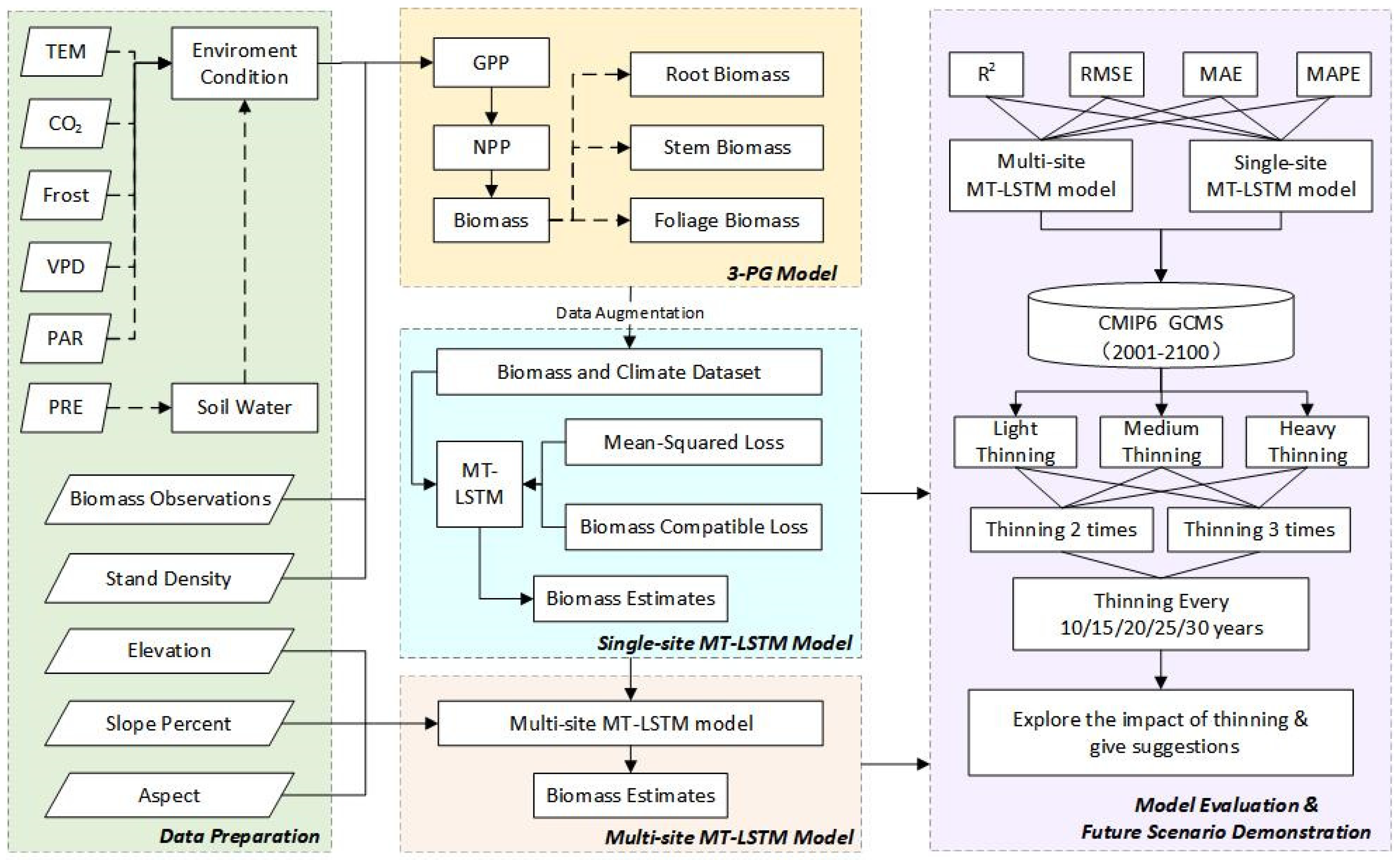
Figure 1. The research framework of this study. In the Data Preparation section, TEM, VPD, PAR, PRE represent temperature, saturated water vapor pressure difference, photosynthetically active radiation, and precipitation, respectively. In the 3-PG Model section, GPP and NPP represent gross primary productivity and net primary productivity. In the Model Evaluation & Future Scenario Demonstration section, R2, RMSE, MAE, MAPE, and CMIP6 GCMS represent R-square, root mean squared error, mean absolute error, mean absolute percentage error, and global climate models in the Coupled Model Intercomparison Project (Phase 6), respectively.
Forests 14 01482 g001
Figure 2. Thinning regimes and time. The horizontal axis represents the year. The vertical axis represents different thinning regimes. 10Y, 15Y, 20Y, 25Y, and 30Y represent the intervals of 10, 15, 20, 25, and 30 years with respect to forest stand thinning, respectively. L, M, H represent light (10%), moderate (20%), and heavy (30%) thinning intensity, respectively, which are distinguished by different colors in the figure; 2T/3T represent simulated thinning two times and three times within the set thinning period.
Forests 14 01482 g002
Figure 3. Taking the Solling site as an example, (a) comparison of the prediction results of the traditional 3-PG model and the staged 3-PG model. Among them, the 3-PG simulation and 3-PG staged simulation are estimated values after optimizing the physiological and ecological parameters of the model using all observation data and stages, respectively. Observation is the value of the observation data. The black dashed line indicates that the stand was thinned in its corresponding year; (b) the changes in the optimal value of the main sensitive parameters—PF20, PRn, and alphaCx—of the 3-PG model at different stages (stand density).
Forests 14 01482 g003
Figure 4. Residual distribution and significance analysis of three models in different sites. (ac) represent the results obtained from training at the Solling site, Hyytiala site, and Bily Kriz site, while (d) represents the results obtained from training on data from all three sites combined. Asterisks refer to the significant differences in the models’ residuals (NS, no significant difference; *, p < 0.05; **, p < 0.01; ***, p < 0.001).
Forests 14 01482 g004
Figure 5. 3PG-MT-LSTM model evaluation results. (ad) represent the results obtained from training at the Solling site, Hyytiala site, Bily Kriz site, and all three sites combined. Different colors represent different evaluation indicators. It should be noted that the unit of RMSE is 10 t.
Forests 14 01482 g005
Figure 6. The future Norway spruce stand’s mean diameter at breast height and biomass trends at the Bily Kriz site. (a,b) show the average diameter at breast height and biomass variation trend of the Norway spruce in 2040, 2060, 2080, and 2100 under several climate scenarios and 18 thinning strategies. Sections (c,d) identify the five most effective thinning techniques, based on the average diameter at breast height and biomass estimations of the forest stand in the year 2100. Where (i) represents the value difference between SSP1-2.6 and SSP5-8.5 scenarios, and (ii) Indicates the difference in values between SSP2-4.5 and SSP5-8.5 scenarios. The presented data display the simulated values of stand diameter at breast height and biomass for various thinning techniques in the years 2040, 2060, 2080, and 2100, arranged in a left-to-right formation.
Forests 14 01482 g006
Table 1. Basic information of biomass data.
SiteLongitude and LatitudeElevation (m)a Forest Age Range (Years)b Forest Biomass Range (t/hm2)c Number of Thinning
Bily Kriz18°19′ E, 49°18′ N87516–3434.49~147.673
Hyytiala24°17′ E, 61°50′ N18534–50128.86~201.781
Solling9°34′ E, 51°45′ N50885–133250.67~372.964
a Forest Age Range refers to the age of the forest stand from the first to the last field survey conducted in the experimental plot. b Forest Biomass Range refers to the maximum and minimum values of forest biomass obtained during the survey and does not represent the biomass of the plot at the minimum (maximum) forest age. c Number of Thinning refers to the number of times the plot was artificially thinned during the entire survey process and does not include density changes caused by natural thinning.
Disclaimer/Publisher’s Note: The statements, opinions and data contained in all publications are solely those of the individual author(s) and contributor(s) and not of MDPI and/or the editor(s). MDPI and/or the editor(s) disclaim responsibility for any injury to people or property resulting from any ideas, methods, instructions or products referred to in the content.