Abstract
The identification of the main factors influencing forest diversity, including both direct and indirect effects, as well as the compatibility of different-level approaches, is a key topic in community ecology and biogeography. The aim of the current study is to assess the contributions of natural and anthropogenic factors to forest diversity in the Moscow region (Russia). This study is based on a quantitative analysis of the linkage between forest diversity and biotopic local factors (LFs) at a lower spatial level, using geobotanical relevés, and external factors (EFs) at an upper spatial level, based on global environmental databases. The classification of 1040 field relevés (including forest-forming tree species, moisture conditions, and soil nutrients) resulted in the identification of eight forest types. A nonmetric multidimensional scaling algorithm, ANOVA post hoc test, hierarchical clustering, and multiple regression analysis were used in data processing. LFs are calculated based on complete species lists using Ellenberg ecological scales. According to a Duncan’s test, LFs provided significant differences between the eight forest types (p < 0.05). At the upper spatial level, the linkage between forest diversity and EFs was most pronounced for climatic factors, soil properties, and topography, including annual mean temperature, soil carbon, clay particle content, and DEM (elevation and slope). The contribution of anthropogenic factors was significantly smaller compared to the natural EFs in the study region.
1. Introduction
The assessment of vegetation diversity is an important objective in botanical and environmental monitoring studies [1,2]. The causes of the current spatial and temporal heterogeneity of vegetation cover are the subject of long-standing discussions due to the uncertainty of the factors determining its diversity. In international practice, there is no contradiction regarding the role of the natural factors of vegetation differentiation (climate variables, topography, geology, hydrology) [3,4], while the significance of anthropogenic factors continues to be debated and refined [5,6,7,8,9]. An improved knowledge of the links between key environmental factors and vegetation cover status is vital in managing ecosystems in the future [10,11,12]. Identifying these links is challenging; the heterogeneity of natural ecosystems, successional dynamics [13], and the interactions between species in communities must be taken into account [14].
New opportunities to identify the macroecological drivers of the spatial heterogeneity of vegetation cover have emerged in the era of readily available remote sensing (RS) and “big data” [15]. It has become necessary to use field survey data to assess typological diversity at high-resolution scales [16]. A common trend in ecological–geographical research methodology is the implementation of quantitative methods for combined field and RS data including global environmental databases (GEDs) [17,18]. The potential of using GEDs is to improve the assessment of the development conditions and current state of forest cover. Diversity of spatial data (WorldClim, ENVIREM, CHELSA, SoilGrids, SRTM, etc.) make it possible to establish the patterns of the spatial and temporal dynamics of forest cover [19] and identify its leading natural and anthropogenic factors [20]. Multiorigin and multidirectional vectors of influence are especially pronounced in age-old development regions. The relevance of local and regional studies of natural communities’ anthropogenic modifications on the basis of GEDs increases in the vicinity of large megacities [21].
For the Moscow region (MR), the largest metropolis in Eastern Europe, the significance of forest cover is extremely important as a source of ecosystem services including the community diversity and species richness of flora and fauna. The combined effect of natural and anthropogenic factors makes the MR enormously complex. In recent decades, the region has experienced intensive urban and road network development and recreational use, which have been accompanied by a strong transformation of forests. At the same time, forests of the MR have been classified as protected. Consequently, a restriction on industrial logging has provided some preservation and the possibility of the spontaneous regeneration of forest cover on former agricultural lands.
Our hypothesis is that macroecological factors (climate, relief, etc.) have a determining influence on the composition and spatial distribution of forests in the region compared to anthropogenic factors. The main aim of this study is to assess the contribution of natural and anthropogenic factors to forest typological diversity in the MR. The objectives of this work are as follows: (1) the classification of field relevés; (2) analysis of the relationship between forest diversity and local factors (LFs) based on Ellenberg ecological scales within the field relevés; (3) analysis of the relationship between forest diversity and external environmental factors (EFs) at the upper spatial level using GEDs; and (4) assessment of the driving factors affecting forest diversity. This study is based on a quantitative analysis of the linkage between forest typological diversity, local factors (LFs) within field relevés, and external environmental factors (EFs) at the upper spatial level using GEDs.
2. Materials and Methods
2.1. Study Area
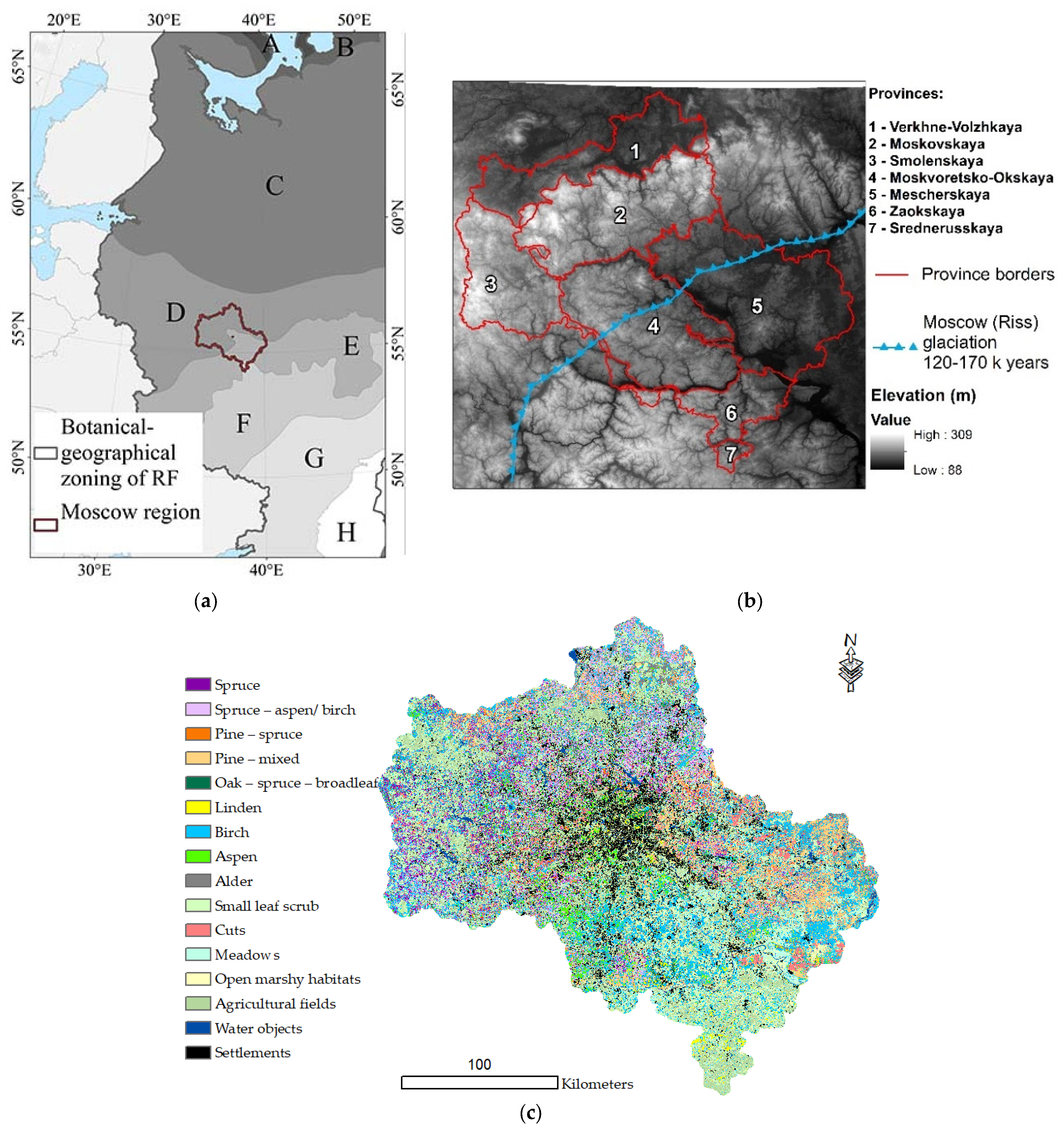
The MR is located in the central part of the East European Plain (Russian)—35°10′–40°15′ E, 54°12′–56°55′ N; its area is 4.7 million ha. This region is characterized by a significant diversity of natural conditions, with several important botanical and geographical boundaries, determined by climatic gradients and the combination of moraine and water–glacial Quaternary deposits. The detailed characteristics of the region are presented in Table A1. The MR is classified as temperate continental according to the map of the climatic regions of Europe [22]. The average annual temperature is 2.7–3.8 °C, and precipitation is 560–640 mm [23]. The topography of the area is generally gentle hilly, with elevations ranging from 90 to 320 m, averaging 174 m, and an average slope of 2.06° (0–30.9°).
The MR is located in the coniferous–broad-leaved (North)/broad-leaved (South–East) forest zones and forest–steppe (far South), where agricultural lands occupy the major part of the area according to the geobotanical map [24,25,26] (Figure 1a, Table A1).
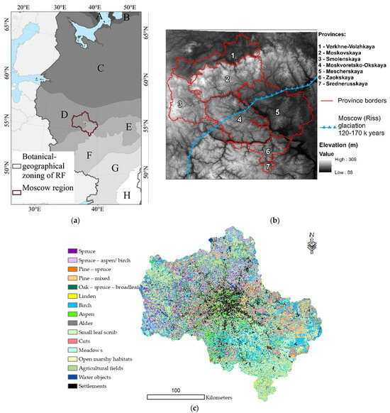
Figure 1.
Study area (a) and vegetation zones [24]: A—tundra; B—forest–tundra; C—coniferous forests; D—coniferous–broad-leaf forests; E—broad-leaf forests; F—forest–steppe; G—steppe; H—semi-desert. DEM and MR provinces (see Table A1) (b) and vegetation map of the MR (c) [25].
The central part of the East European Plain and the territory of the region have a long history of land use. Forests are cut down and plowed, and in some years, the forest area amounted to about a quarter of the total area of the territory. Since the beginning of the 20th century, the forest cover in the MR has nearly doubled due to reforestation efforts. Additionally, as former agricultural lands are converted into fallow lands, natural reforestation is actively underway. Currently, the forest cover in the MR exceeds 50%, with no primary forests remaining [25,27]. Most of the forests are old-growth and second-growth, resembling primary forests in terms of tree and undergrowth composition but differing significantly in stand age structure. As a result, the forest cover in the MR is represented by a successional mosaic of forests with varying composition, age, and origin. Coniferous and mixed forests include a significant proportion of reforested areas [28].
2.2. Study Design
The study is based on the integration of field data and GEDs. This approach has been previously tested to evaluate the typological diversity of the MR forest vegetation [29]. The study was divided into 5 steps:
- Field studies;
- Classification of forest types;
- Estimation of local factors (LFs) and external factors (EFs);
- Linkage between forest types and EFs/LFs;
- Assessment of the driving factors of forest diversity.
The effect of environmental factors was analyzed at two spatial levels: (i) local factors (LFs): biotope properties (plant species composition based on Ellenberg ecological scales) within the locations of field relevés and (ii) external (supracenotic) factors (EFs) on a grid with a spatial resolution of 90–250 m and 1000 m: climatic, morphometric variables, soil properties, and anthropogenic impact. A correlation approach was used to find linkages between LFs/EFs and forest properties, as well as a nonmetric multidimensional scaling algorithm, ANOVA post hoc test, hierarchical clustering, and multiple regression analysis using the STATISTICA 12 software application.
2.3. Classification of Field Data and Assessment of Forest Biodiversity
Typology Classification
The total number of fields relevés is 1140. A complete species composition and vertical structure were recorded. Species coverage is given in percentage. When distinguishing layers, the following designation was adopted: A—tree layer (generative and senile trees) subdivided into two sublayers (A1 and A2) depending on stand structure; B—undergrowth (virginial trees—B1) and shrub layer (virginial and generative shrubs 1–10 m high—B2); C—herbaceous-shrub layer (including immature individuals of trees and shrubs below 1 m); D—moss layer. Mosses were counted only as part of the D layer. The area of the field relevés is 400 m2. We tried to exclude forest communities with active successional processes, so relevés were selected for the period 2009–2022.
It is essential to determine the optimal set of syntaxons (forest types) with a sufficient level of significance appropriate to the spatial scale of the study area when assessing typological diversity. In this regard, the ecological–phytocenotic method was used to classify the relevés [30]. This method shows a good correspondence between typological and mapped units, aligns with Russian forest typology units, maintains a clear hierarchy of units, and considers rare forest community types in contrasting biotopic conditions.
A map of 11 forest formations and 31 association groups was developed in a previous stage of the research [25] (Figure 1c). In earlier studies, the classification was refined to generalize the data while considering the relationship between formation classes and environmental conditions. Additionally, intrazonal communities were identified (pine swamps, small-leaf swamps, and alder forests), which differ from communities in automorphic habitats primarily due to soil conditions. The full species composition of vascular plants and mosses was used in the analysis of community composition.
The validation (clarification of relevés’ affiliation with forest community types) and visualization of the classification were performed using hierarchical clustering with Ward’s minimum variance method in STATISTICA 12 and NMDS ordination in the R statistical programming environment [31].
2.4. LF Estimation Using Field Data
We calculated the LFs for each relevé based on Ellenberg ecological scales [32] using Juice software 7.0 [33], taking into account the cover of each species (weighted by species cover) in each layer of the community.
We obtained a quantitative profile of forest types through their LF values: temperature (T), soil reaction (R), soil moisture (M), soil nitrogen fertility (N), and light (L). Essentially, we are referring to the properties of ecological niches (ENs) specific to the typological units we selected. The use of the EN concept at the superspecies level aligns with Hutchinson’s understanding [34], who defined niche as the set of environmental states within which a species can survive, within a multidimensional space. Thus, the values of habitat condition factors at the relevé points are used as LFs, including for overlaying vectors in the ordination space to estimate environmental gradients.
2.5. EF Estimation Using GEDs
All external spatial variables (EFs) were checked for the normality of their distribution using a chi-square test, considering critical values for a probability level of 0.05 and degrees of freedom. To address collinearity between the original predictors, we excluded some variables from the analysis if their correlation was below 0.75 in absolute value and their significance level was less than 0.05, based on the Pearson correlation coefficient.
2.5.1. Climate Variables
To assess the influence of environmental factors, we analyzed the relationship between the distribution of forest types and bioclimatic variables using the WorldClim database (spatial resolution of 1 km × 1 km) [35]. Out of the full set of 19 bioclimatic variables, 4 that affect forest vegetation composition were selected based on the Pearson correlation coefficient:
- T ann—annual mean temperature (bio01);
- T cold Q—mean temperature of coldest quarter (bio11);
- P ann—annual precipitation (bio12);
- P wet M—precipitation of wettest month (bio13).
2.5.2. Soil Cover Variables
Soil parameters at 10 cm depth were taken from the SoilGrids database (spatial resolution of 250 m) [36]. From the full set of physical and chemical indicators, four were selected as noncorrelated:
- Soil moist—soil water content at 33 kPa (field capacity) at 10 cm depth [37];
- Soil pH—soil pH in H2O at 10 cm depth [38];
- Soil clay—clay content in % (kg/kg)—proportion of clay particles (<0.002 mm) in the fine earth fraction, g/kg [39];
- Soil carb—soil organic carbon content g/kg [39].
2.5.3. Digital Elevation Model Variables
Two morphometric variables—elevation and slope—were extracted from the SRTM 90 m DEM (Digital Elevation Model) dataset [40].
2.5.4. Anthropogenic Variables
The anthropogenic impact luminosity of the Earth’s surface was assessed using the geographical location of the points and remote sensing data on nighttime lights, specifically the VIIRS monthly and annual moonlight-adjusted nighttime lights [41]. Nighttime luminosity is highly correlated with the consumption of primary energy resources at the regional level [42] and indicates several parameters of anthropogenic load, including population density, recreational use, and atmospheric pollution. The following independent variables were used:
- Light ann—night illumination (W·cm−2·sr−1);
- Dist light—distance to objects with illumination over 100 W·cm−2·sr−1;
- Dist center—distance to the center of Moscow;
- Dir center—azimuth from Moscow (south was taken as 0 degrees).
2.6. Relationship between LFs and EFs
The values of each factor (both LFs and EFs) were compared for the 8 forest types. This allowed us to identify the significant differences between each pair of forest types for each factor using an ANOVA followed by a post hoc Duncan’s test. The software STATISTICA 12 was used for this analysis.
The nonmetric multidimensional scaling (NMDS) ordination of relevés (complete species lists with percentages for each relevé) was performed using square root transformation and Wisconsin double standardization with Bray–Curtis distance in the R 4.2.2 statistical programming environment to analyze the distribution of forest types in the multidimensional space of environmental conditions [31]. The NMDS ordination algorithm is well-suited for obtaining accurate results in large datasets with strong noise (random variation) [43] and is well-established in the analysis of plant communities [44].
LFs allow for a precise evaluation of forest types. By comparing the direction of factors with the ordination axes in ecological space, we can identify the leading factors influencing forest composition diversity. To evaluate the relationship between LFs and EFs, we performed the ordination of geobotanical relevés with the overlay of passive LF and EF vectors on the NMDS ordination space. The direction and length of LF and EF vectors reveal their interrelationships as well as their correlation with the primary environmental factors (NMDS1 and NMDS2).
2.7. Driving Factors of Forest Diversity
A multiple regression analysis was performed to identify the relationship between biotopic-level forest cover variability factors (LFs), expressed through species scores using Ellenberg ecological scales, and external remote sensing variables (EFs) at the upper spatial level.
3. Results
3.1. Results of Classification
Eight forest types were identified based on the dominant tree species and varying habitat conditions: 1—Spruce forests (Sp), formed by Picea abies (459 relevés); 2—Pine forests (P)—Pinus sylvestris (210 relevés); 3—Pine swamp forests (Pp)—Pinus sylvestris (46 relevés); 4—Broad-leaf forests (Bl)—Tilia cordata, Quercus robur, occasionally with Acer platanoides (136 relevés); 5—Small-leaf forests (Sl)—Betula pendula, B. pubescens, Populus tremula (188 relevés); 6—Small-leaf swamp forests (Slp)—B. pendula, B. pubescens (26 relevés); 7—Gray alder forests (GAl)—Alnus incana (24 relevés); 8—Black alder forests (BAl)—Alnus glutinosa (51 relevés). Each forest type is represented by communities with different combinations of common dominant species in the tree layer. Syntaxa are identified based on the predominant ecological and morphological plant groups in the subordinate layers, which depend on habitat moisture and nutrients (Table 1). Consequently, mesophytic groups, as well as eutrophic grass–marsh and oligotrophic shrub–sphagnum communities, are distinguished within the vegetation of the subordinate layers.

Table 1.
Classification of forest types.
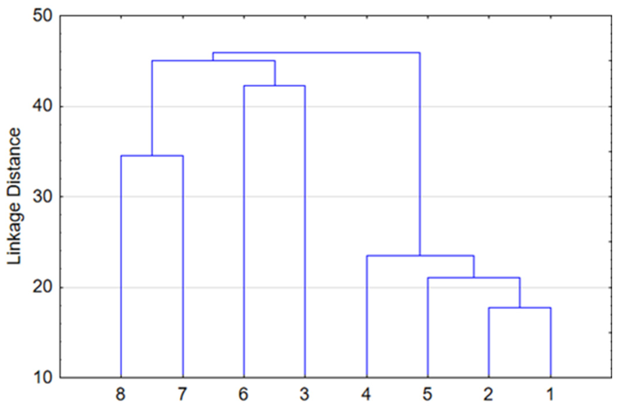
Hierarchical clustering was performed to illustrate the similarity of forest types in terms of floristic composition. The mean percentage of each species within each of the eight forest types was calculated. Based on these data, the Ward method and Euclidean distance squared were applied using STATISTICA 12. Forest types in the lower topography with increased moisturization are well-separated at the upper level (Figure 2). This includes eutrophic grass–marsh communities such as gray alder and black alder forests (#7,8), as well as oligotrophic shrub–sphagnum communities such as pine and small-leaf forests (#3,6). Another group is characterized by zonal spruce and pine forests (#1,2), as well as mesophytic broad-leaf and small-leaf communities (#4,5) found in automorphic positions. At the lower level, species composition homogeneity is naturally observed in coniferous and deciduous forests in automorphic positions.
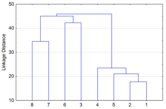
Figure 2.
Hierarchy cluster analysis of forest structure.
3.2. Differences of Forest Types by LFs
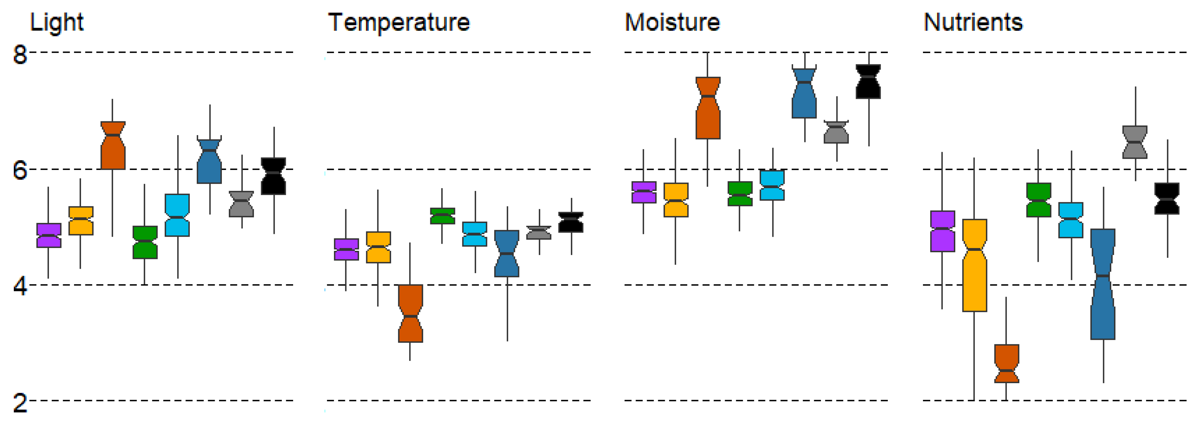
The distribution of identified forest types according to LF differences is shown in Figure 3. Different forest types are well differentiated by light (L). Spruce forests (#1) and broad-leaf forests (#4) are associated with a low illumination in the understory, while sparse pine swamp forests (#3) and small-leaf swamp forests (#6) are associated with a high illumination under the canopy. This differentiation is well explained by the shade tolerance of the tree species and the heliophilic nature of the shrub and ground-layer plants in these communities (Figure 3).
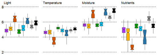
Figure 3.
Boxplots of LF variation in forest types with mean values: median, hinges: 1st and 3rd quartile; whisker: largest value no further than 1.5 interquartile ranges; notch: 95% confidence interval. Forest types: 1—spruce, 2—pine, 3—pine swamp, 4—broad-leaf, 5—small-leaf, 6—small-leaf swamp, 7—gray alder, 8—black alder.
Coniferous and broad-leaf forests generally correspond to natural patterns. In particular, coniferous forests, typical for the northwestern sector of the MR (Figure 1) with colder mean annual temperatures, are well distinguished by the temperature (T). On the contrary, broad-leaf forests are in the range of high values, which is also well-explained based on their zonal position in the southeastern sector of the region. The small range of values in broad-leaf forests (oak and linden) indicates a strict preference for a rather narrow range of temperature regime. The wide range of mean error values in small-leaf swamp forests (#6) indicates a high ecological plasticity in terms of temperature regime. The intrazonal status of the latter confirms this statement (Figure 3).
The soil moisture (M) variable discriminates forest types into two supratypes quite accurately. Three forest types—pine swamp and small-leaf forests (#3,6) and black alder forests (#8)—prefer humid conditions. Forest types #1, 2, 4, and5 are less dependent on soil moisture (Figure 3).
The lowest soil reaction (R) is in pine swamp forests (#3), and the average is found in spruce and pine forest types (#1,2), as well as small-leaf and black alder forests (#5,8). The high values of soil reaction (with the highest pH values) correspond to the broad-leaf and gray alder forests (#4,7). The distribution of forest types according to the soil reaction factor correlates well with soil nutrients (N) (r = 0.87) (Figure 3).
According to the Duncan’s test, most pairs of forest types differ significantly (p < 0.05) in all LF parameters. The exceptions are as follows: (1) small-leaf forests (#5) do not differ from pine forests (#2) and gray alder forests (#7) with respect to light (L), gray alder forests (#7) and black alder forests (#8) do not differ in temperature (T), black alder forests (#8) do not differ in soil reaction (R), and spruce forests (#1) do not differ in soil nitrogen (N); (2) spruce forests (#1) do not differ from pine forests (#2) in temperature (T), broad-leaf forests (#4) in light (L), and black alder forests (#8) in soil nitrogen (N); (3) Pine swamp forests (#3) do not differ from small-leaf swamp forests (#6) in soil reaction (R) and soil moisture (M), broad-leaf forests (#4) do not differ from small-leaf swamp forests (#6) and pine swamp forests (#3) in soil moisture (M).
3.3. Differences in Forest Types by EFs
3.3.1. Climatic Variables
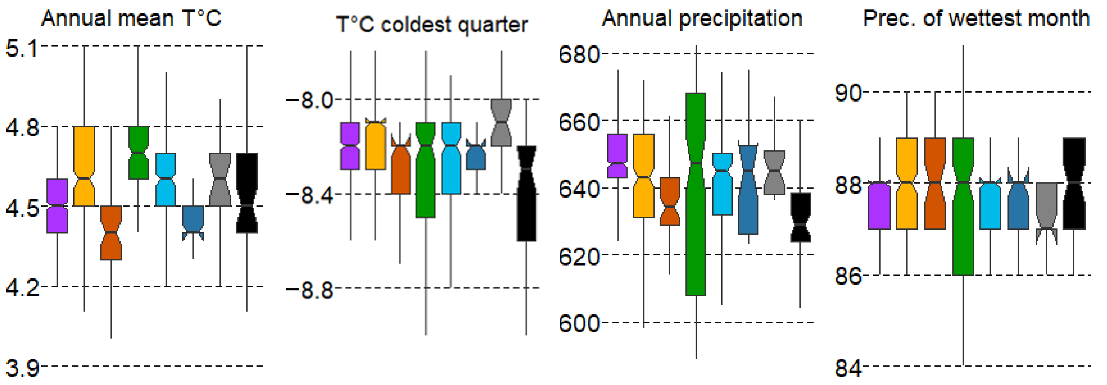
The gradient of variation in the mean values of the climatic variables is rather small, with the error variation spread indicating the presence of a wide range of individual forest types under different conditions. The most contrasting forest types along the gradient of mean annual temperature (T ann) are spruce forests (#1), as well as pine swamp and small-leaf swamp forests (#3,6), distributed in the range of lower temperatures, while broad-leaf communities (#4) are confined to higher T ann values (Figure 4).
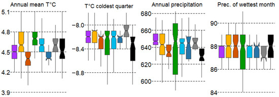
Figure 4.
Boxplots of climatic variable variation in forest types with mean values: median, hinges: 1st and 3rd quartile; whisker: largest value no further than 1.5 interquartile ranges; notch: 95% confidence interval. Forest types: 1—spruce, 2—pine, 3—pine swamp, 4—broad-leaf, 5—small-leaf, 6—small-leaf swamp, 7—gray alder, 8—black alder.
The differences in the mean values of the variable mean annual temperature (T ann) for most forest types are significant according to the Duncan’s test, with the exception that pine forests (#2) do not differ from small-leaf forests (#5) and alder forests (#7,8). Spruce forests (#1) also do not differ from pine swamp forests (#3) and small-leaf swamp forests (#6). This may suggest that many spruce forests are plantations and may not align with their ecological optimum regarding climatic factors. The high values of the temperature of the coldest quarter of the year (T cold Q) are typical for gray alder forests (#7), while low values are characteristic of black alder forests (#8). The other forest types do not differ significantly from each other (Figure 4). Mean annual precipitation (P ann) shows the widest range in broad-leaf and small-leaf communities (#4,6), with significant differences most pronounced in type #4. Gray alder communities (#7) also significantly differ from other types in terms of precipitation in the wettest month (P sub wet M) (Figure 4).
The gradient of variation in the mean values of the climatic variables is relatively small, with error variation indicating a wide range of conditions under which individual forest types occur. The most contrasting forest types along the gradient of mean annual temperature (T ann) are spruce forests (#1), as well as pine swamp forests (#3) and small-leaf swamp forests (#6), which are distributed within the lower temperature range. In contrast, broad-leaf communities (#4) are confined to higher T ann values (Figure 4).
3.3.2. Soil Variables
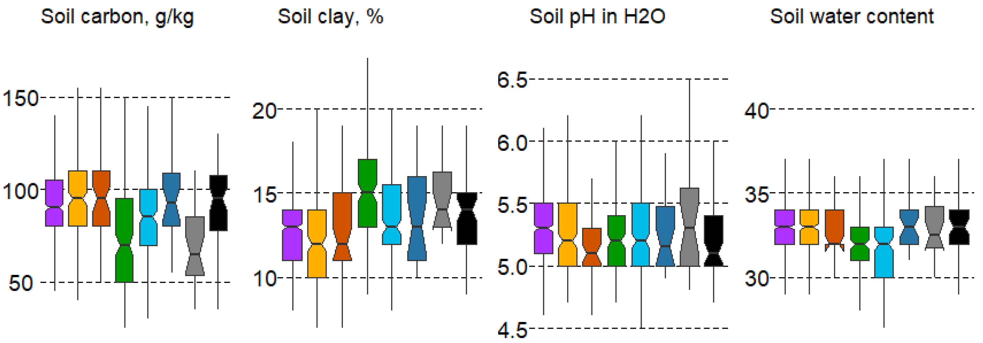
The analysis of the linkage between forest types and soil variables revealed major differences in soil clay content and weaker differences in soil pH, according to the Duncan’s test. Despite the complexity and heterogeneity of soil composition, some regularities in the distribution of forest types by soil variables in the 10 cm soil layer were identified (Figure 5).
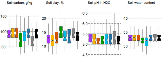
Figure 5.
Boxplots of soil variable variation in forest types with mean values: median, hinges: 1st and 3rd quartile; whisker: largest value no further than 1.5 interquartile ranges; notch: 95% confidence interval. Forest types: 1—spruce, 2—pine, 3—pine swamp, 4—broad-leaf, 5—small-leaf, 6—small-leaf swamp, 7—gray alder, 8—black alder.
Soil carbon content is significantly lower in broad-leaf (#4) and gray alder forests (#7). Soil clay content is highest in habitats #4 and7. The minimum content is in spruce and pine forests (#1,3), as well as broad-leaf and gray alder forests (#7), which significantly differ. In terms of soil water content, broad-leaf (#4) and small-leaf forests (#5) differ significantly (minimal compared to most formations). In terms of soil moisture pH, significant differences are observed for gray alder forests (#7), whose pH value is slightly acidic (Figure 5).
3.3.3. Terrain Variables
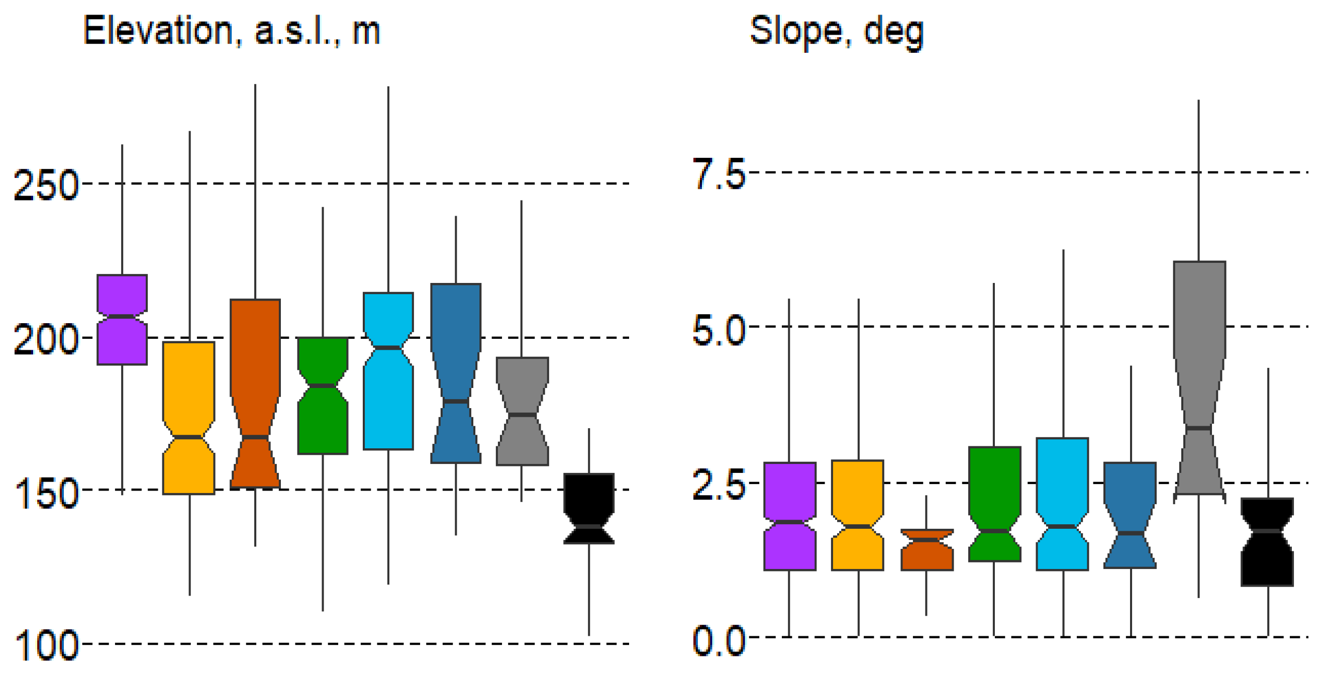
Despite the relatively flat terrain of the study area, differences in altitude and slope were significant for forest types (according to the Duncan’s test) and were especially evident in the boxplots for the altitude variable (Figure 6).

Figure 6.
Boxplots of terrain variable variation in forest types with mean values: median, hinges: 1st and 3rd quartile; whisker: largest value no further than 1.5 interquartile ranges; notch: 95% confidence interval. Forest types: 1—spruce, 2—pine, 3—pine swamp, 4—broad-leaf, 5—small-leaf, 6—small-leaf swamp, 7—gray alder, 8—black alder.
In terms of elevation, spruce forests (#1) are significantly higher than all other forest types, while black alder communities (#8) are typically found in low-relief areas. Regarding slope, gray alder forests (#7) show the most noticeable differences, as they are often located along the slopes of brooks and rivers.
3.3.4. Anthropogenic Variations
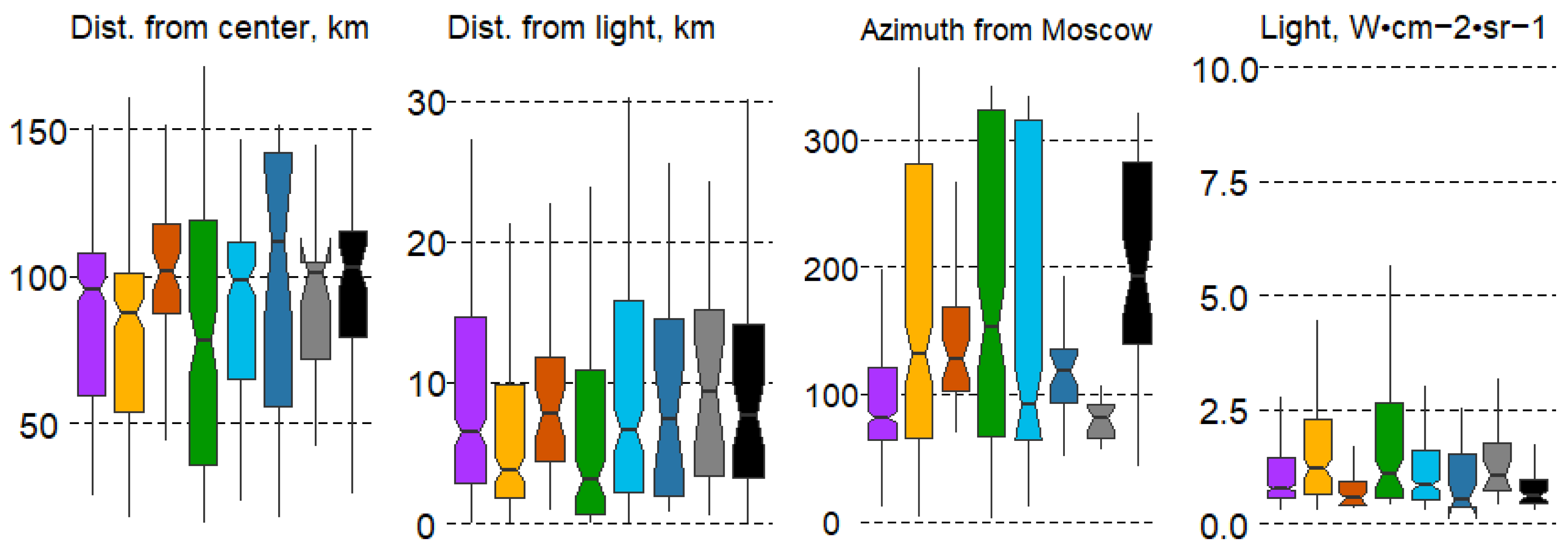
Significant differences in the distance to the center of Moscow were observed only in some forest types, specifically pine and broad-leaf forests (#2,4). Intrazonal communities showed the least significant differences, including pine and small-leaf swamp forests (#3,6) and black alder communities (#8). Broad-leaf (#4) and small-leaf swamp forests (#6) exhibited the greatest range of variation (Figure 7).
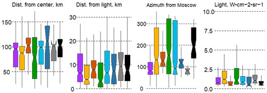
Figure 7.
Boxplots of anthropogenic impact variation in forest types with mean values: median, hinges: 1st and 3rd quartile; whisker: largest value no further than 1.5 interquartile ranges; notch: 95% confidence interval. Forest types: 1—spruce, 2—pine, 3—pine swamp, 4—broad-leaf, 5—small-leaf, 6—small-leaf swamp, 7—gray alder, 8—black alder.
The distance from large settlements does not significantly affect the spatial distribution of forest types. In contrast, the direction from the center of Moscow has a major impact on forest type variation. Differences are significant in almost all forest types. Spruce forests (#1) are confined to the western part of the region, pine and small-leaf swamp forests (#3,6) are typical in the northwestern and northern sectors, gray alder forests (#7) are found strictly in the west, and black alder forests (#8) are typical for the eastern part of the MR. The remaining forest types have a wider distribution across the MR. Nighttime lights (Light ann) significantly differ only for broad-leaf forests (#4), which are more frequently located closer to large cities and often form artificial forest parks (Figure 7).
3.4. Assessment of the Driving Factors of Forest Biodiversity
Now we need to determine which driving factors most significantly influence forest diversity and whether our assumption that climate variables play a greater role among external factors (EFs) is correct. To address this, we first apply the nonmetric multidimensional scaling (NMDS) algorithm for ordination.
We represented forest types through quantitative LF values by relating species to biotopic factors (T, R, M, N, and L) based on Ellenberg scales. Using NMDS ordination, we analyzed the location of relevés in a system of abstract axes with overlapping passive LF vectors. The distinguished forest types are quite clearly distributed in the ordination space (Figure 8a). The NMDS1 axis is associated with changes in soil nutrients (N) and soil reaction (R) (changing from rich broad-leaf forests to poor pine communities and oligotrophic bogs with acidic soil reaction), and the NMDS2 axis is associated with soil moisture (M) (from spruce and pine forests to black and gray alder forests) and lightness (L). All factors are related significantly to the distribution of relevés in the ordination space, but the highest squared correlation coefficient is observed with R (r2 = 0.83), N (r2 = 0.69), and L (r2 = 0.64), less with T (r2 = 0.52) and M (r2 = 0.51). Thus, we can quantitatively characterize eight forest types by the properties of their inherent ecological niches.
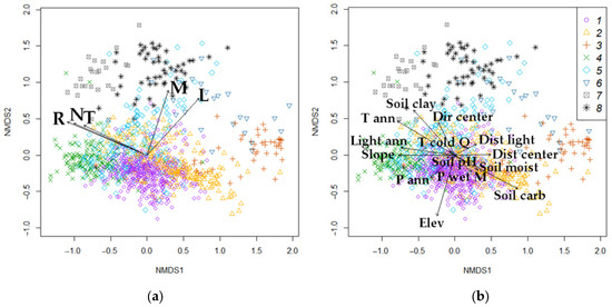
Figure 8.
NMDS ordination: (a)—by LFs (T—temperature, R—soil reaction, M—soil moisture, N—soil nitrogen fertility, and L—light); (b)—by EFs. Forest types: 1—spruce, 2—pine, 3—pine swamp, 4—broad-leaf, 5—small-leaf, 6—small-leaf swamp, 7—gray alder, 8—black alder.
Similarly, the relationship between EFs and the composition of forest types is visualized in the ordination space by overlapping the passive vectors of external factors (Figure 8b). The correlation of these factors with the two axes is also quite high, as in the case of LFs. All climatic parameters, anthropogenic impact (except Dir center), soil carbon content, and slope are (more than 0.70) correlated with the NMDS1 axis (change in T, R, and N) the most. NMDS2 (change in M) has the closest relationship with elevation and soil clay content. The relationship with soil moisture pH is not significant (Pr(>r) = 0.93). Thus, a significant relationship is observed with almost all EFs except two (T cold Q and Soil pH), which can be explained by the heterogeneity of the soil cover (Table 2).
Table 2.
Correlation of the distribution of relevés with ordination axes and squared correlation coefficients with LFs and EFs.
We compare the ordination plots with LFs and EFs and estimate the direction and length of the vectors (factors) with environmental significance (Figure 8a,b). We selected from EFs the variables having r2 > 0.3 (Figure 8b). The leading EFs are mean annual temperature, slope, soil carbon, and clay particle content. Most coincidences of vector directions and lengths along the NMDS1 axis occur in the pairing of temperature characteristics (T–T ann) and soil richness (N–Soil clay). On the NMDS2 axis, to a lesser extent, the coincidence occurs in the pairs M–P ann and M–P wet M.
From the analysis above, it is evident that the linkage between forest types and local factors (LFs) is stronger than with external factors (EFs). Forest types exhibit more significant differentiation based on LF variables (as shown by the Duncan’s test). Additionally, the correlation between LF vectors and ordination axes is higher, with squared correlation coefficients (r2) being significantly greater for LFs than for EFs. In contrast, EFs show high variability in their influence on forest types.
A multiple regression analysis was performed to identify the influence of the driving factors on the variability in forest types. The set of LFs characterizing the properties of the ecological niche of certain forest types was consistently evaluated in relation to the whole complex of external natural and anthropogenic factors (EFs). The analysis revealed a significant relationship between nearly all LFs and the climatic variables, as well as terrain features, especially elevation. Soil variables, such as the proportion of clay particles and carbon content, showed weaker associations. Among the anthropogenic factors, the distance from Moscow had the most notable impact: it is positively related to moisture content (M), light conditions (L), and temperature (T). Additionally, the direction from the center is positively associated with temperature (T). Other factors showed much weaker correlations with LFs (Table 3). Overall, the determination coefficients (R2) were significant but relatively low in most cases.
Table 3.
Multiple regression analysis of the relationship between LFs and EFs.
4. Discussion
Our study confirms that the composition and functioning of natural systems are predominantly influenced by natural factors, including regional and local climate, topography, tree species composition, and local flora [45,46,47,48]. However, the combined impact of major natural and anthropogenic factors, particularly across different spatial scales, has not been thoroughly explored in the literature. Given the importance of understanding how forest cover relates to key environmental factors, we aimed to provide a comprehensive analysis of both natural and anthropogenic influences.
Climatic variables are the most significant among EF. Bioclimatic variables explain ecological and physiological processes that determine the distribution of plants which is confirmed by a number of studies [49,50]. The most pronounced factor of spatial distribution of the major forest types is mean annual temperature (T ann). Broad-leaf communities have the largest range of mean annual precipitation (P ann). These results demonstrate natural patterns: the MR is located in the ecotone area, where we observe the transition of coniferous–broad-leaf to broad-leaf forest zone with a difference in mean annual temperature in the latitudinal direction of about 1 °C on average and the sum of annual precipitation of about 730 mm [51].
Warming and moisturizing effect of Moscow indirectly impacts forest composition of MR [23]. The abovementioned patterns are confirmed by recent map of forest typology [25,30].
Despite a long history of environmental management, the forests of MR have retained the essential features of native broad-leaf–coniferous forests. These features include a diverse mix of tree species, a multilayered community structure, and rich typological and species diversity [28,45]. We investigated the differences in forest typology by analyzing local factors (LFs) at geobotanical relevé points and external factors (EFs) at a broader, supracentric level. This approach allowed us to evaluate how various forest types relate to these factors across different spatial scales. Our analysis consistently revealed significant differences among forest types in relation to both natural and anthropogenic factors.
Previous studies in the central part of the Russian Plain revealed the optimal habitats of spruce forests (with Picea abies) on the leveled parts and gentle slopes of the moraine hills of watershed plateaus with podzolic loamy soils, as well as on the ridge hills of fluvioglacial plains with weakly podzolic sandy loam soils [45]. Most spruce forests originate as a short-derivative stage of native spruce forests on clearcuts as a result of both spontaneous succession and the process of spruce silviculture [52,53,54]. Obviously, the artificial origin of a large part of spruce forests in the MR shifts the native properties of the ecological niche [28]. Nevertheless, spruce forests (#1) prefer low light, reduced soil moisture, and low values of temperature, soil reaction, and soil nutrients (Figure 3). Spruce forests are significantly confined to elevated terrain and watersheds (Figure 6) with lower mean annual temperatures (T ann) (Figure 4), which corresponds to their predominance in the forest cover of the northern part of the MR [25]. Spruce communities are also found in the southern part of the MR along river valleys [55] as a silviculture, including old, largely decayed trees [56].
Pine forests (with Pinus sylvestris) (#2) occupy mainly fluvioglacial upland watersheds, and to a lesser extent—well drained depressions and surrounding upland and transitional bogs. These communities may originate after human impact—in silviculture or on burnings that occur quite regularly in these landscapes [57]. Among LFs, there is a significant difference between spruce and pine forests in nutrition. Similarly, among EFs, pine forests are not separated significantly from small-leaf (#5) and alder forests (#7,8) by T ann, which means a eurytopic habitat preference. Most of the pine forests have almost no pine undergrowth; instead, the spruce is presented in the second tree layer. Spruce gradually becomes part of the canopy and provides diverse-age undergrowth. In other cases, a subnemoral composition of pine forests with an undergrowth of hazel and broad-leaf species takes place.
Pine swamp forests (#3) are often found in runoff hollows, watershed depressions, and moraine–fluvioglacial landscapes. The distribution of oligotrophic pine swamp forests differs from pine on well-drained substrates (#2) by the adaptation of ground-layer species to the best conditions of light (L), moisture (M), and soil reaction (pH), as well as low temperature (T) and soil richness (N) (Figure 3). Oligotrophic pine swamp forests have lower temperatures among the EFs (Figure 4). A floristic core with a large number of typical species additionally indicates the maturity of communities and a strict confinement to oligotrophic habitats [58]. Numerous studies based on instrumental measurements [59,60] confirm this pattern of pine swamp communities.
Broad-leaf forests (with Tilia cordata and Quercus robur) grow on the most fertile soils [61], so they often are cut for agricultural land. In this regard, they are found in small fragments, increasing in presence in the southeast of the MR. Broad-leaf forests occupy the highest soil clay level and higher mean annual temperatures (T ann). They prefer soils with a neutral reaction and increased nutrition (Figure 3).
Small-leaf forests (with Betula pendula, B. pubescens, Populus tremula) (#5) dominate in the MR mainly due to the growth of young stands on clearcuts, and in recent decades with regenerative succession on abandoned agricultural lands. Most of the birch and aspen forest communities are secondary. They grow in a wide range of environmental conditions; this determines the diversity of small-leaf forests [62,63]. Well-drained small-leaf forests with birch on automorphic positions in the landscape (#5) have a greater number of insignificant differences in the pairs with other community types with respect to biotopic environmental factors (LFs) according to the Duncan’s test.
Small-leaf swamp forests (#6) are derivative communities that replace coniferous forests with longhorn and sphagnum [64,65], as well as during the overgrowth of transitional bogs after fires, which rarely occur in the MR. They occupy small areas in hollows and depressions with a high groundwater table. They are light-demanding (L) and characterized by increased moisture values and poor soil nutrition (N) (Figure 3). Notably, the limiting factor for overwatered small-leaf forests is the precipitation of the wettest month (P wet M).
Gray alder (Alnus incana) and black alder (A. glutinosa) communities with nitrophilic flora (#7,8) are mainly referred to as native forests. Among the LFs, alder forests prefer minimum values for soil moisture (M) and soil reaction (pH) but the highest values for soil richness (N) (Figure 3). Alder eutrophic grass–marsh forests are found throughout the MR. They occupy small areas on the slopes of the floodplain terraces of small rivers and streams, in lake hollows, and in depressions with traces of former watercourses. Native gray alder forests stretch in narrow strips along the valleys of rivers and temporary watercourses, while derived ones are associated with the restoration of cut forests in habitats with a close groundwater table. Terrain variables are particularly good at distinguishing between gray alder forests, located mainly on slopes, and black alder forests (in depressions). According to the climatic variables, alder forests are characterized by a low temperature of the coldest quarter of the year (T cold Q) (Figure 4).
The analysis of the differences between forest types in terms of the variables characterizing anthropogenic impact showed a significant difference with only one indicator—the direction from the center of Moscow. In this case, it is rather a coupled relationship between this indicator and the climatic variables, which reflects the latitudinal distribution of coniferous and mixed forests to the northwest and broad-leaf forests to the southeast, which is consistent with our MR vegetation map [25,65] and, in general, with the botanical and geographic zoning of the territory [24,26]. To test the indirect influence of the anthropogenic factor on the composition of communities, its correlation with the climatic indicator T ann was evaluated using the Dist center variable for the territory of the southern sector. The correlation coefficient was significant, r = −0.46, indicating a synergistic effect of both factors, in which the role of the climatic variable clearly prevails.
In general, there is a lower accuracy of EF variables to estimate forest diversity compared to LFs. In our case, this may be explained by the difference in the spatial resolution of variables, as EFs at upper level have a 90, 250, and 1000 m resolution, while LFs have a 30–60 m resolution. In addition, the quality of the relationship with external predictors is complicated by the peculiarities of the region’s forest cover, which is highly fragmented (especially stand patterns) due to a long history of economic development and a large area of coniferous crops.
5. Conclusions
The composition and spatial distribution of forest types are shaped by a combination of environmental factors. Through the analysis of species composition, we assessed the local biotopic characteristics (LFs) of forest types and evaluated the significance of key external variables (EFs) in shaping forest diversity around the megacity of Moscow, Russia. At the local level, the most significant factors influencing forest types are soil acidity, nutrient levels, and light conditions. On a broader spatial scale, climatic factors played a crucial role in forest cover variability, with average annual temperature and precipitation being the most significant. Topography, including elevation and slope steepness, also had a notable impact on forest composition. Among the soil variables, carbon and clay content are the most influential in determining forest variability, though they are only weakly correlated with LFs. Anthropogenic factors, such as the proximity to populated areas and the distance from Moscow, are less significant in comparison to natural factors. The stronger correlation between LFs and community composition compared to EFs can be attributed to the finer spatial resolution of local factors. Despite a long history of resource use in the area, the forests continue to exhibit the primary characteristics of native broad-leaf–coniferous forests, including a diverse stand composition, multilayered community structure, and rich species diversity.
Author Contributions
Conceptualization, methodology, funding acquisition, writing—original draft, T.C.; data curation, writing—review and editing, N.B.; visualization, investigation, validation, software, I.K.; resources, A.N. All authors have read and agreed to the published version of the manuscript.
Funding
The core of this study was conducted under the Russian Science Foundation (RSF) project (№ 24-17-00120) regarding data processing and analysis. Field data collection was supported by the state research task (FMWS-2024-0007 No. 1021051703468-8) of the Institute of Geography RAS.
Data Availability Statement
Data are available upon request.
Acknowledgments
The authors thank the many colleagues who participated in the collection of the primary material, among whom the proportion in relevés was E.G. Suslova, E.V. Tikhonova, O.A. Pesterova, N.G. Kadetov, O.V. Morozova, M.A. Arkhipova, and S.Yu. Popov.
Conflicts of Interest
The authors declare no conflicts of interest.
Appendix A
Table A1.
General properties of the physiographic provinces of the Moscow region: values in the table are means ± SD [28].
Table A1.
General properties of the physiographic provinces of the Moscow region: values in the table are means ± SD [28].
| Provinces | |||||||
|---|---|---|---|---|---|---|---|
| Verkhnevolzhskaya | Moskovskaya | Smolenskaya | Moskvoretsko-Okskaya | Mescherskaya | Zaokskaya | Srednerusskaya | |
| #1 | #2 | #3 | #4 | #5 | #6 | #7 | |
| Number of glaciations | 4 | 3 | 3 | 2–3 | 2–3 | 2 | 2 |
| Climate | |||||||
| Tavg jan (°) | −9.65 ± 0.69 | −9.16 ± 0.6 | −8.94 ± 0.57 | −8.27 ± 0.29 | −8.78 ± 0.52 | −8.85 ± 0.22 | −8.63 ± 0.09 |
| Tavg july (°) | 17.49 ± 0.21 | 17.47 ± 0.37 | 17.25 ± 0.28 | 18.10 ± 0.42 | 18.79 ± 0.32 | 18.52 ± 0.27 | 18.50 ± 0.1 |
| Annual precipitation (mm) | 637 ± 9.96 | 652 ± 9.62 | 636 ± 9.81 | 621 ± 21.5 | 614 ± 27.47 | 574 ± 9.46 | 558 ± 3.88 |
| Precipitation of warmest month (mm) | 86.2 ± 2.03 | 87.6 ± 1.64 | 84.6 ± 0.78 | 84.6 ± 1.03 | 86.9 ± 2.53 | 82.3 ± 1.31 | 79.0 ± 0.65 |
| Relief | |||||||
| Elevation (m) | 146.7 ± 18.6 | 206.8 ± 29.47 | 213.1 ± 30.92 | 174.4 ± 25.63 | 133.5 ± 16.80 | 168.6 ± 29.86 | 176.4 ± 23.46 |
| Slope (°) | 3.54 ± 2.74 | 5.18 ± 3.81 | 4.85 ± 3.73 | 4.49 ± 3.5 | 3.74 ± 2.88 | 4.58 ± 3.59 | 3.75 ± 2.89 |
| Surface Deposits, Soils, and Vegetation | |||||||
| Deposits | Outwash, moraine–fluvioglacial, shale loam and sands, underlain by limestones or clays | Moraine, moraine–fluvioglacial loam and sands | Moraine loam, fluvioglacial and limno–fluvioglacial loams and sands | Moraine and moraine–fluvioglacial loams and sands | Fluvioglacial, ancient alluvial sands and loams | Shale loess-type loams on moraine and fluvioglacial sands | Shale and moraine, fluvioglacial loams on rock outcrops |
| Soil | Sod–podzolic, gleyic soils | Sod–podzolic, gleyic, wetland soils | Sod–podzolic soils | Sod–podzolic, Light gray forest soils | Sod-podzolic, Podzolic gleyic, Wetland soils | Gray forest, light gray forest soils | Gray forest soils |
| Forests | Birch–pine, spruce–aspen/birch | Broad-leaved–spruce, spruce–aspen/birch | Broad-leaved–spruce, spruce–aspen/birch | Aspen/birch | Spruce—oak—pine, Birch-pine | Aspen/birch, Aspen/birch–broad-leaved | Oak |
References
- Chytrý, M. Vegetation of the Czech Republic: Diversity, Ecology, History and Dynamics. Preslia 2012, 84, 427–504. [Google Scholar]
- Patel, N.N.; Angiuli, E.; Gamba, P.; Gaughan, A.; Lisini, G.; Stevens, F.R.; Tatem, A.J.; Trianni, G. Multitemporal Settlement and Population Mapping from Landsat Using Google Earth Engine. Int. J. Appl. Earth Obs. Geoinf. 2015, 35, 199–208. [Google Scholar] [CrossRef]
- Bailey, R.G. Identifying Ecoregion Boundaries. Environ. Manag. 2004, 34, S14–S26. [Google Scholar] [CrossRef] [PubMed]
- Carvalho, M.C.; Gomide, L.R.; Santos, R.M.d.; Scolforo, J.R.S.; Carvalho, L.M.T.d.; Mello, J.M. Modeling Ecological Niche of Tree Species in Brazilian Tropical Area. CERNE 2017, 23, 229–240. [Google Scholar] [CrossRef]
- Dramstad, W.; Sogge, C. Agricultural Impacts on Landscapes: Developing Indicators for Policy Analysis. In Proceedings of the NIJOS/OECD Expert Meeting on Agricultural Landscape Indicators, Oslo, Norway, 7–9 October 2002; NIJOS-Rapport. Norwegian Institute for Soil and Forest Mapping: Akershus, Norway, 2003. [Google Scholar]
- Mücher, C.A.; Klijn, J.A.; Wascher, D.M.; Schaminée, J.H. A New European Landscape Classification (LANMAP): A Transparent, Flexible and User-Oriented Methodology to Distinguish Landscapes. Ecol. Indic. 2010, 10, 87–103. [Google Scholar] [CrossRef]
- Tishkov, A.A. Actual Biogeography as a Methodological Basis for Biodiversity Conservation. Quest. Geogr. 2012, 134, 15–57. [Google Scholar]
- Van Eetvelde, V.; Antrop, M. Landscape Character beyond Landscape Typology: Methodological Issues in Trans-Regional Integration in Belgium. In Proceedings of the 18th International Annual ECLAS Conference: Landscape assessment, from theory to Practice: Applications in Planning and Design, Belgrade, Serbia, 10–14 October 2007; University of Belgrade: Belgrade, Serbia, 2007; pp. 229–239. [Google Scholar]
- Winkler, K.; Fuchs, R.; Rounsevell, M.; Herold, M. Global Land Use Changes Are Four Times Greater than Previously Estimated. Nat. Commun. 2021, 12, 2501. [Google Scholar] [CrossRef]
- Balmford, A.; Bond, W. Trends in the State of Nature and Their Implications for Human Well-Being. Ecol. Lett. 2005, 8, 1218–1234. [Google Scholar] [CrossRef]
- Fassnacht, F.E. About the Link between Biodiversity and Spectral Variation. Appl. Veg. Sci. 2022, 25, e12643. [Google Scholar] [CrossRef]
- Loreau, M.; Hector, A. Partitioning Selection and Complementarity in Biodiversity Experiments. Nature 2001, 412, 72–76. [Google Scholar] [CrossRef]
- Kiseleva, V.; Stonozhenko, L.; Korotkov, S. The dynamics of forest species composition in the eastern Moscow region. Folia For. Pol. 2020, 62, 53–67. [Google Scholar] [CrossRef]
- Ammer, C.; Fichtner, A.; Fischer, A.; Gossner, M.M.; Meyer, P.; Seidl, R.; Thomas, F.M.; Annighöfer, P.; Kreyling, J.; Ohse, B.; et al. Key Ecological Research Questions for Central European Forests. Basic Appl. Ecol. 2018, 32, 3–25. [Google Scholar] [CrossRef]
- Hijmans, R.J.; Cameron, S.E.; Parra, J.L.; Jones, P.G.; Jarvis, A. Very High Resolution Interpolated Climate Surfaces for Global Land Areas. Int. J. Climatol. 2005, 25, 1965–1978. [Google Scholar] [CrossRef]
- Zhang, X.; Liu, L.; Chen, X.; Xie, S.; Gao, Y. Fine Land-Cover Mapping in China Using Landsat Datacube and an Operational SPECLib-Based Approach. Remote Sens. 2019, 11, 1056. [Google Scholar] [CrossRef]
- Döpper, V.; Panda, S.; Waigl, C.; Braun, M.; Feilhauer, H. Using Floristic Gradient Mapping to Assess Seasonal Thaw Depth in Interior Alaska. Appl. Veg. Sci. 2021, 24, e12561. [Google Scholar] [CrossRef]
- Rocchini, D.; Lenoir, J.R.M.H. Remote Sensing at the Interface between Ecology and Climate Sciences. Meteorol. Appl. 2021, 28, e2022. [Google Scholar] [CrossRef]
- Pshegusov, R.K.; Tembotova, F.A.; Sablirova, Y.M. The Main Regularities of the Spatial Localization of Various Types of the Coniferous and Coniferous-Deciduous Forests of the North Macroslope of Western Caucasus by Earth Remote Sensing Materials. For. Sci. Issues 2019, 2, 1–11. [Google Scholar] [CrossRef]
- Akinyemi, F.; Tlhalerwa, L.; Eze, P. Land Degradation Assessment in an African Dryland Context Based on the Composite Land Degradation Index and Mapping Method. Geocarto Int. 2019, 36, 1838–1854. [Google Scholar] [CrossRef]
- Potere, D.; Schneider, A.; Angel, S.; Civco, D.L. Mapping Urban Areas on a Global Scale: Which of the Eight Maps Now Available Is More Accurate? Int. J. Remote Sens. 2009, 30, 6531–6558. [Google Scholar] [CrossRef]
- Rivas-Martínez, S.; Penas, A.; Díaz, T. Biogeographic Map of Europe; Cartographic Service University of León: León, Spain, 2004. [Google Scholar]
- Litvinenko, L.N.; Kalinina, A.A. Raspredelenie Osadkov Na Territorii Moskovskoj Oblasti Pri Nalichii i Otsutstvii Krupnogo Antropogennogo Obrazovanija (Distribution of Precipitation on the Territory of the Moscow Region in the Presence and Absence of a Large Anthropogenic Formation). Ecol. Urban. Areas 2018, 2, 66–71. [Google Scholar] [CrossRef]
- Kurnaev, S.F. Lesorastitel’noe Rajonirovanie SSSR (Forest Zoning of the USSR); Nauka: Moscow, Russia, 1973. [Google Scholar]
- Kotlov, I.; Chernenkova, T. Modeling of Forest Communities’ Spatial Structure at the Regional Level through Remote Sensing and Field Sampling: Constraints and Solutions. Forests 2020, 11, 1088. [Google Scholar] [CrossRef]
- Gribova, S.A.; Isachenko, T.I.; Lavrenko, E.M. Vegetation of European Part of the USSR; Nauka Leningradskoe otd-nie: Leningrad, Russia, 1980. [Google Scholar]
- Abaturov, A.V. Iz istorii lesov Podmoskov’ja (From the history of the forests of the Moscow region). In Dinamika Hvojnyh Lesov Podmoskov’ja (Dynamic of Coniferous Forests of Moscow Region); Nauka: Moscow, Russia, 2000; pp. 22–32. ISBN 5-02-004435-0. [Google Scholar]
- Chernenkova, T.V.; Kotlov, I.P.; Belyaeva, N.G.; Suslova, E.G.; Morozova, O.V.; Pesterova, O.; Arkhipova, M.V. Role of Silviculture in the Formation of Norway Spruce Forests along the Southern Edge of Their Range in the Central Russian Plain. Forests 2020, 11, 778. [Google Scholar] [CrossRef]
- Chernenkova, T.; Kotlov, I.; Belyaeva, N.; Suslova, E. Spatiotemporal Modeling of Coniferous Forests Dynamics along the Southern Edge of Their Range in the Central Russian Plain. Remote Sens. 2021, 13, 1886. [Google Scholar] [CrossRef]
- Chernenkova, T.V.; Morozova, O.V. Classification and Mapping of Coenotic Diversity of Forests. Contemp. Probl. Ecol. 2017, 10, 738–747. [Google Scholar] [CrossRef]
- R Core Team (2020)—European Environment Agency. Available online: https://www.eea.europa.eu/data-and-maps/indicators/oxygen-consuming-substances-in-rivers/r-development-core-team-2006 (accessed on 19 April 2024).
- Ellenberg, H.; Weber, H.E.; Düll, R.; Wirth, V.; Werner, W.; Paulissen, D. Zeigerwerte von Pflanzen in Mitteleuropa. Scr. Geobot. 1991, 18, 248. [Google Scholar]
- Tichý, L. JUICE, Software for Vegetation Classification. J. Veg. Sci. 2002, 13, 451–453. [Google Scholar] [CrossRef]
- Hutchinson, G.E. Concluding Remarks. Cold Spring Harb. Symp. Quant. Biol. 1957, 22, 415–427. [Google Scholar] [CrossRef]
- Fick, S.E.; Hijmans, R.J. WorldClim 2: New 1-Km Spatial Resolution Climate Surfaces for Global Land Areas. Int. J. Climatol. 2017, 37, 4302–4315. [Google Scholar] [CrossRef]
- Batjes, N.H.; Ribeiro, E.; van Oostrum, A. Standardised Soil Profile Data to Support Global Mapping and Modelling (WoSIS Snapshot 2019). Earth Syst. Sci. Data 2020, 12, 299–320. [Google Scholar] [CrossRef]
- Hengl, T.; Gupta, S. Soil Water Content (Volumetric %) for 33kPa and 1500 kPa Suctions Predicted at 6 Standard Depths (0, 10, 30, 60, 100 and 200 Cm) at 250 m Resolution. Zenodo 2019. [Google Scholar] [CrossRef]
- Hengl, T. Soil pH in H2O at 6 Standard Depths (0, 10, 30, 60, 100 and 200 Cm) at 250 m Resolution. Zenodo 2018. [Google Scholar] [CrossRef]
- Hengl, T.; Wheeler, I. Soil Organic Carbon Content in x 5 g/Kg at 6 Standard Depths (0, 10, 30, 60, 100 and 200 Cm) at 250 m Resolution. Zenodo 2018. [Google Scholar] [CrossRef]
- CGIAR-CSI 2017; SRTM 90m Digital Elevation Database. CGIAR Platform for Big Data in Agriculture: Palmira, Colombia.
- Wang, Z.; Shrestha, R.; Yao, T.; Kalb, V. Black Marble User Guide (Version 1.2). Available online: https://ladsweb.modaps.eosdis.nasa.gov/missions-and-measurements/viirs/VIIRS_Black_Marble_UG_v1.2_April_2021.pdf (accessed on 4 March 2022).
- Tronin, A.A.; Gornyy, V.I.; Kritsuk, S.G.; Latypov, I.S. Nighttime lights as a quantitative indicator of anthropogenic load on ecosystems. Curr. Probl. Remote Sens. Earth Space 2014, 11, 237–244. [Google Scholar]
- Minchin, P.R. An Evaluation of the Relative Robustness of Techniques for Ecological Ordination. In Theory and Models in Vegetation Science, Proceedings of the Symposium, Uppsala, Sweden, 8–13 July 1985; Prentice, I.C., van der Maarel, E., Eds.; Springer: Dordrecht, The Netherlands, 1987; pp. 89–107. ISBN 978-94-009-4061-1. [Google Scholar]
- Saccone, P.; Pyykkonen, T.; Eskelinen, A.; Virtanen, R. Environmental Perturbation, Grazing Pressure and Soil Wetness Jointly Drive Mountain Tundra toward Divergent Alternative States. J. Ecol. 2014, 102, 1661–1672. [Google Scholar] [CrossRef]
- Rysin, L.P.; Savel’eva, L.I. Elovye Lesa Rossii (Spruce Forests of Russia); Nauka: Moscow, Russia, 2002; ISBN 5-02-006501-3. [Google Scholar]
- Sang, W.; Bai, F. Vascular Diversity Patterns of Forest Ecosystem before and after a 43-Year Interval under Changing Climate Conditions in the Changbaishan Nature Reserve, Northeastern China. In Forest Ecology; Van Der Valk, A.G., Ed.; Springer: Dordrecht, The Netherlands, 2008; pp. 115–130. ISBN 978-90-481-2794-8. [Google Scholar]
- Cornwell, W.K.; Grubb, P.J. Regional and Local Patterns in Plant Species Richness with Respect to Resource Availability. Oikos 2003, 100, 417–428. [Google Scholar] [CrossRef]
- Zhang, P.; Chen, D.; Linderholm, H.W.; Zhang, Q. How Similar Are Annual and Summer Temperature Variability in Central Sweden? Adv. Clim. Change Res. 2015, 6, 159–170. [Google Scholar] [CrossRef]
- Pshegusov, R.H.; Chadaeva, V.A. Ecological Niche Modeling of Galinsoga Ruiz et Pav. Species in the Native and Caucasian Part of the Invasive Ranges. Russ. J. Biol. Invasions 2022, 13, 245–258. [Google Scholar] [CrossRef]
- Title, P.O.; Bemmels, J.B. ENVIREM: An Expanded Set of Bioclimatic and Topographic Variables Increases Flexibility and Improves Performance of Ecological Niche Modeling. Ecography 2018, 41, 291–307. [Google Scholar] [CrossRef]
- Annenskaya, G.N.; Zhuchkova, V.K.; Kalinina, V.R.; Mamai, I.I.; Nizovtsev, V.A.; Khrustaleva, M.A.; Tseselchuk, Y.N. Landscapes of the Moscow Region and Their Current State; SGU: Smolensk, Russia, 1997. [Google Scholar]
- Nitsenko, A.A. On the Study of the Ecological Structure of the Vegetation Cover. Bot. Z. 1969, 54, 1002–1014. [Google Scholar]
- Ogureeva, G.N.; Miklyaeva, I.M.; Suslova, E.G.; Shvergunova, L.V. (Eds.) Vegetation of Moscow Region (Rastitel’nost’ Moskovskoj Oblasti); EKOR: Moscow, Russia, 1996. [Google Scholar]
- Tømmerås, B. Skogens Naturlige Dynamikk. Elementer Og Prosesser i Naturlig Skogutvikling. DN-Rapp. 1994, 5, 1–47. [Google Scholar]
- Rysin, L.P. Lesa Yuzhnogo Podmoskov’ya (Forests of Southern Part of Moscow Region); Nauka: Moscow, Russia, 1985. [Google Scholar]
- Szydlarski, M.; Modrzyński, J.; Stopiński, M.; Majewski, M.; Maras, K. Comparing Natural Regeneration of Norway Spruce Picea abies (L.) Karst in the Kaszuby Lake District and in the Other Regions of Northern Poland (Porównanie Naturalnego Odnowienia Świerka Pospolitego Picea abies (L.) Karst. na Pojezierzu Kaszubskim i w Innych Regionach Północnej Polski); Instytut Badawczy Leśnictwa (Forest Research Institute): Sękocin Stary, Poland, 2018. [Google Scholar] [CrossRef]
- Suslova, E.G. Forests of Moscow Region. Ecosyst. Ecol. Dyn. 2019, 3, 119–190. [Google Scholar]
- Chernenkova, T.V.; Suslova, E.G.; Morozova, O.V.; Belyaeva, N.G.; Kotlov, I.P. Biodiversity of forests in the Moscow region. Ecosyst. Ecol. Dyn. 2020, 4, 60–144. [Google Scholar] [CrossRef]
- Frolova, G.; Frolov, P.V.; Shanin, V.N.; Ivanova, N. Analysis of Factors Affecting the Regeneration of Major Forest-Forming Species in the Pine Forests of the Southern Moscow Region. For. Sci. Issues 2019, 2, 1–27. [Google Scholar] [CrossRef]
- Wyka, T.; Oleksyn, J.; Zytkowiak, R.; Karolewski, P.; Jagodziński, A.; Reich, P. Responses of Leaf Structure and Photosynthetic Properties to Intra-Canopy Light Gradients: A Common Garden Test with Four Broadleaf Deciduous Angiosperm and Seven Evergreen Conifer Tree Species. Oecologia 2012, 170, 11–24. [Google Scholar] [CrossRef] [PubMed]
- Kurnaev, S.F. Osnovnye Tipy Lesa Srednej Chasti Russkoj Ravniny (Main Forest Types of Russian Plain Middle Part); Nauka: Moscow, Russia, 1968. [Google Scholar]
- Abaturov, Y.D.; Zvorykina, K.V.; Ilyushenko, A.F. Tipy Berezovyh Lesov Central’noj Chasti Juzhnoj Tajgi (Types of Birch Forests of the Central Part of the Southern Taiga); Nauka: Moscow, Russia, 1982. [Google Scholar]
- Vasilevich, V.I. Upland birch forests in North-West of European Russia. Bot. Z. 1996, 81, 1–13. [Google Scholar]
- Nitsenko, A.A. Typology of Small-Leaved Forests in the European Part of the USSR; Leningrad University Publishing House: Leningrad, Russia, 1972. [Google Scholar]
- Kotlov, I.; Chernenkova, T.; Belyaeva, N. Urban Forests of Moscow: Typological Diversity, Succession Status, and Fragmentation Assessment. Landsc. Ecol. 2023, 38, 3767–3789. [Google Scholar] [CrossRef]

Disclaimer/Publisher’s Note: The statements, opinions and data contained in all publications are solely those of the individual author(s) and contributor(s) and not of MDPI and/or the editor(s). MDPI and/or the editor(s) disclaim responsibility for any injury to people or property resulting from any ideas, methods, instructions or products referred to in the content. |
© 2024 by the authors. Licensee MDPI, Basel, Switzerland. This article is an open access article distributed under the terms and conditions of the Creative Commons Attribution (CC BY) license (https://creativecommons.org/licenses/by/4.0/).