


A Preliminary System of Equations for Predicting Merchantable Whole-Tree Volume for the Decurrent Non-Native Quercus rubra L. Grown in Navarra (Northern Spain)

 ,
,  ,
,  and
and
Abstract
1. Introduction
2. Materials and Methods
2.1. Data
2.2. Taper Equation
2.3. Merchantable Whole-Tree Volume
2.4. Model Fitting
3. Results
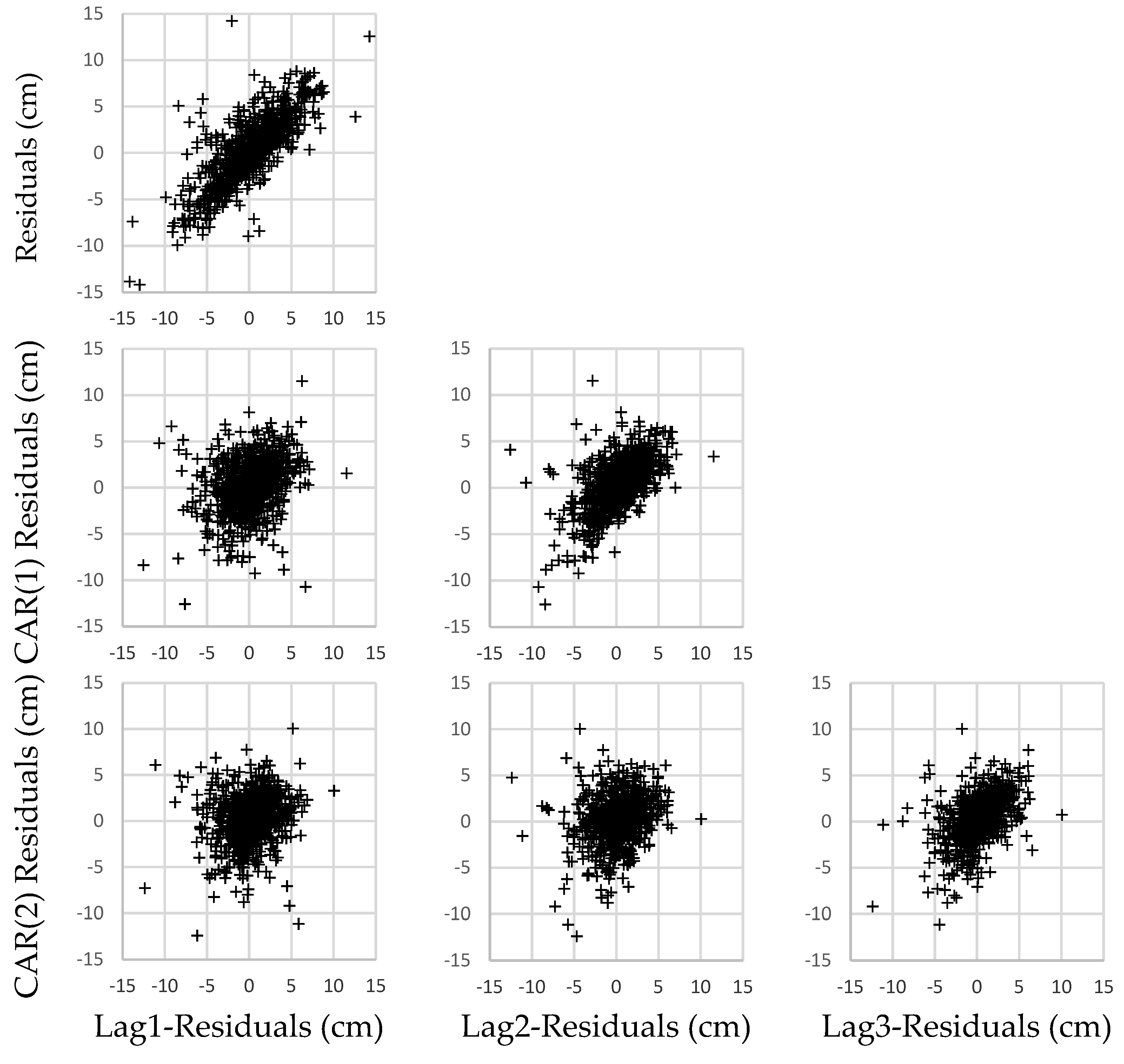
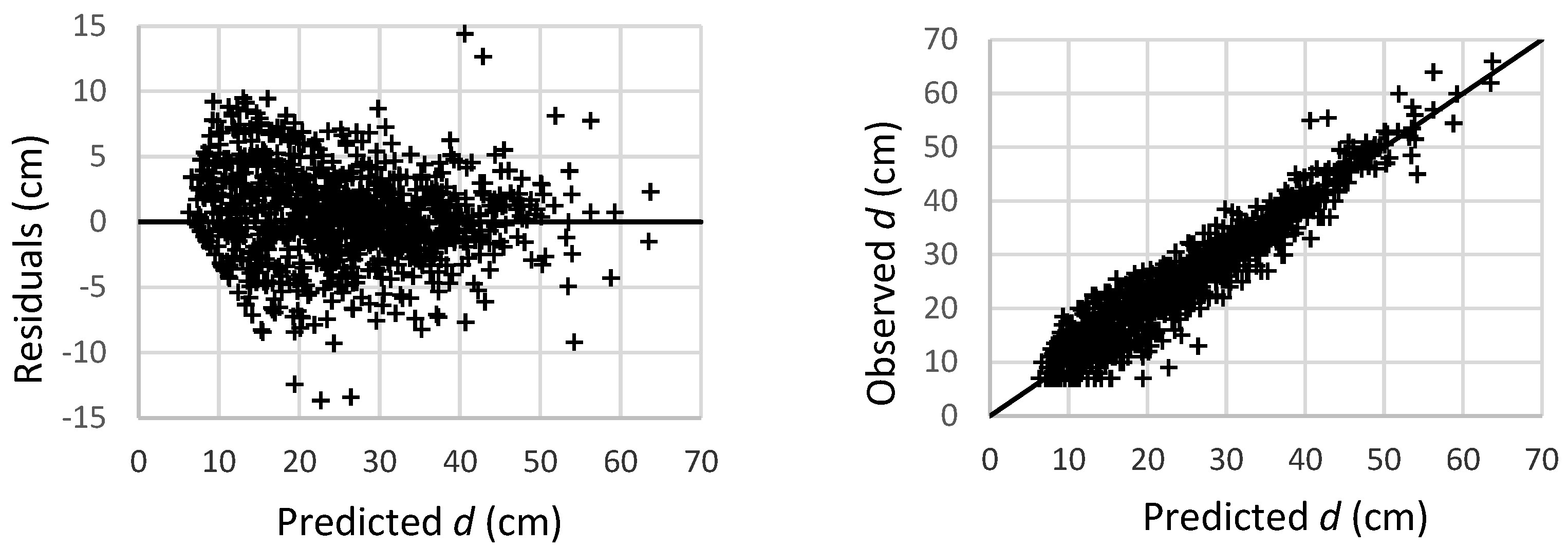
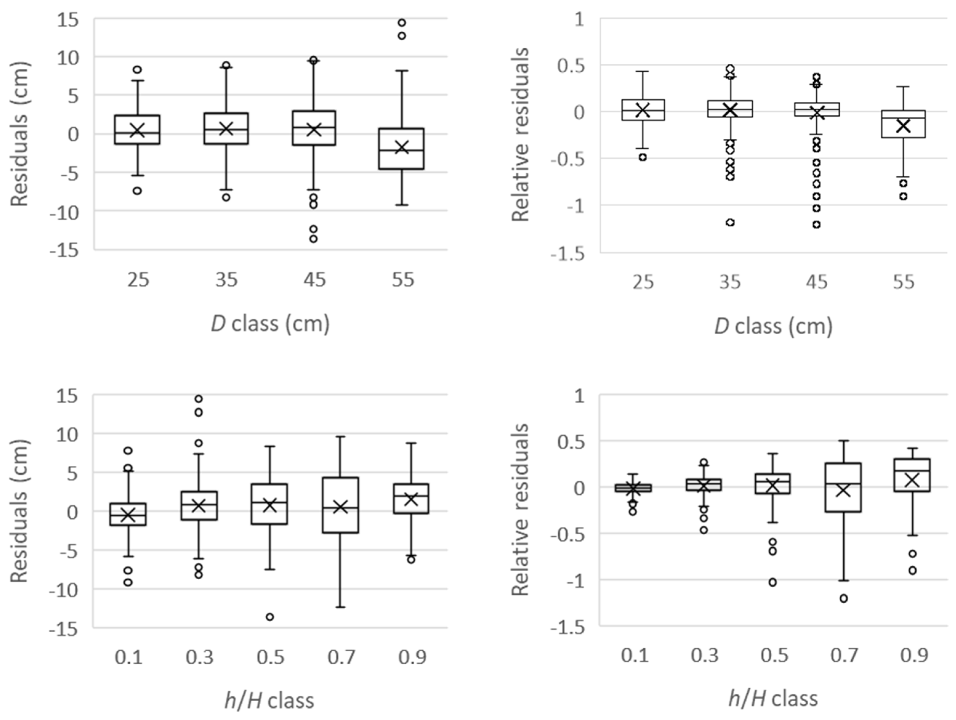
3.1. Taper Equation
3.2. Merchantable Whole-Tree Volume
3.3. System of Equations
4. Discussion
5. Conclusions
Author Contributions
Funding
Data Availability Statement
Acknowledgments
Conflicts of Interest
References
- Clutter, J.L.; Fortson, J.C.; Pienaar, L.V.; Brister, G.H.; Bailey, R.L. Timber Management: A Quantitative Approach; Krieger Publishing Company: New York, NY, USA, 1983. [Google Scholar]
- Avery, T.E.; Burkhart, H.E. Forest Measurements, 5th ed.; McGraw-Hill: New York, NY, USA, 2002. [Google Scholar]
- Assmann, E. The Principles of Forest Yield Study; Pergamon Press: Oxford, UK, 1970. [Google Scholar]
- Burkhart, H.E.; Tomé, M. Modeling Forest Trees and Stands; Springer: New York, NY, USA, 2012. [Google Scholar]
- MacFarlane, D.W.; Weiskittel, A.R. A new method for capturing stem taper variation for trees of diverse morphological types. Can. J. For. Res. 2016, 46, 804–815. [Google Scholar] [CrossRef]
- Adu-Bredu, S.; Bi, A.F.T.; Bouillet, J.-P.; Me, M.K.; Kyei, S.Y.; Saint-Andre, L. An explicit stem profile model for forked and un-forked teak (Tectona grandis) trees in West Africa. For. Ecol. Manag. 2008, 255, 2189–2203. [Google Scholar] [CrossRef]
- MacFarlane, D.W. Allometric scaling of large branch volume in hardwood trees in Michigan, USA: Implications for above-ground forest carbon stock inventories. For. Sci. 2011, 57, 451–459. [Google Scholar] [CrossRef]
- Ver Planck, N.R.; MacFarlane, D.W. Modelling vertical allocation of tree stem and branch volume for hardwoods. Forestry 2014, 87, 459–469. [Google Scholar] [CrossRef]
- Corral-Rivas, J.J.; Vega-Nieva, D.J.; Rodríguez-Soalleiro, R.; López-Sánchez, C.A.; Wehenkel, C.; Vargas-Larreta, B.; Álvarez-González, J.G.; Ruiz-González, A.D. Compatible system for predicting total and merchantable stem volume over and under bark, branch volume and whole-tree volume of pine species. Forests 2017, 8, 417. [Google Scholar] [CrossRef]
- Pemán García, J.; Cosculluela Giménez, J.; Gómez Fernández, J.A. Quercus rubra L. In Producción y Manejo de Semillas y Plantas Forestales; Pemán García, J., Navarro, R., Nicolás, J.L., Prada, M.A., Serrada, R., Eds.; Organismo Autónomo Parques Nacionales, Tomo II: Madrid, Spain, 2013; pp. 292–304. [Google Scholar]
- MITECO. Spanish National Forest Inventory. Available online: https://www.miteco.gob.es/es/biodiversidad/temas/inventarios-nacionales/inventario-forestal-nacional.html (accessed on 7 November 2023).
- Bi, H. Trigonometric variable-form taper equations for Australian eucalyptus. For. Sci. 2000, 46, 397–409. [Google Scholar]
- Max, T.A.; Burkhart, H.E. Segmented polynomial regression applied to taper equations. For. Sci. 1976, 22, 283–289. [Google Scholar]
- Biging, G. Taper equations for second-growth mixed conifers of Nothern California. For. Sci. 1984, 30, 1103–1117. [Google Scholar]
- Daquitaine, R.; Saint-Andre, L.; Leban, J.M. Product Properties Prediction—Improved Utilisation in the Forestry-Wood Chain Applied on Spruce Sawnwood: Modelling Stem Properties Distribution; FAIR CT 96-1915—Final Report Subtask A2.1.: Nancy, France, 1999. [Google Scholar]
- Fang, Z.; Borders, B.E.; Bailey, R.L. Compatible volume-taper models for loblolly and slash pine based on a system with segmented-stem form factors. For. Sci. 2000, 46, 1–12. [Google Scholar] [CrossRef]
- Sharma, M.; Zhang, S.Y. Variable-exponent taper equations for jack pine, black spruce, and balsam fir in eastern Canada. For. Ecol. Manag. 2004, 198, 39–53. [Google Scholar] [CrossRef]
- Kozak, A. My last words on taper functions. For. Chron. 2004, 80, 507–515. [Google Scholar] [CrossRef]
- Hartley, H.O. The modified Gauss-Newton method for the fitting of nonlinear regression functions by least squares. Technometrics 1961, 3, 269–280. [Google Scholar] [CrossRef]
- Draper, N.R.; Smith, H. Applied Regression Analysis, 3rd ed.; Wiley: New York, NY, USA, 1998. [Google Scholar]
- McTague, J.P.; Weiskittel, A. Evolution, history, and use of stem taper equations: A review of their development, application, and implementation. Can. J. For. Res. 2021, 51, 210–235. [Google Scholar] [CrossRef]
- Myers, R.H. Classical and Modern Regression with Applications, 2nd ed.; Duxbury Press: Belmont, CA, USA, 1990. [Google Scholar]
- Ryan, T.P. Modern Regression Methods; John Wiley & Sons: New York, NY, USA, 1997. [Google Scholar]
- Zimmerman, D.L.; Núñez-Antón, V. Parametric modeling of growth curve data: An overview (with discussion). Test 2001, 10, 1–73. [Google Scholar] [CrossRef]
- SAS Institute Inc. SAS/ETS® 9.2 User’s Guide; SAS Institute Inc.: Cary, NC, USA, 2008. [Google Scholar]
- SAS Institute Inc. SAS/STAT® 9.2 User’s Guide, 2nd ed.; SAS Institute Inc.: Cary, NC, USA, 2009. [Google Scholar]
- West, P.W.; Ratkowsky, D.A.; Davis, A.W. Problems of hypothesis testing of regressions with multiple measurements from individual sampling units. For. Ecol. Manag. 1984, 7, 207–224. [Google Scholar] [CrossRef]
- Parresol, B.R.; Vissage, J.S. White Pine Site Index for the Southern Forest Survey; USDA, Forest Service, Southern Research Station, Research Paper SRS-10; USDA: Asheville, NC, USA, 1998. [Google Scholar]
- Kitikidou, K.; Chatzilazarou, G. Estimating the sample size for fitting taper equations. J. For. Sci. 2008, 54, 176–182. [Google Scholar] [CrossRef]
- Gevorkiantz, S.R.; Olsen, L.P. Composite Volume Tables for Timber and Their Application in the Lake States; USDA Technical Bulletin No. 1104; USDA: Washington, DC, USA, 1955. [Google Scholar]
- Neilsen, W.A.; Gerrand, A.M. Growth and branching habit of Eucalyptus nitens at different spacing and the effect on final crop selection. For. Ecol. Manag. 1999, 123, 217–229. [Google Scholar] [CrossRef]
- Kerr, G.; Boswell, R.C. The influence of spring frosts, ash bud moth (Prays fraxinella) and site on forking of young ash (Fraxinus excelsior) in southern Britain. Forestry 2001, 74, 29–40. [Google Scholar] [CrossRef]
- Gomat, H.Y.; Deleporte, P.; Moukini, R.; Mialounguila, G.; Ognouabi, N.; Saya, A.R.; Vigneron, P.; Saint André, L. What factors influence the stem taper of Eucalyptus: Growth, environmental conditions, or genetics? Ann. For. Sci. 2011, 68, 109–120. [Google Scholar] [CrossRef]
- Montagu, K.D.; Duttmer, K.; Barton, C.V.M.; Cowie, A.L. Developing general allometric relationships for regional estimates of carbon sequestration and example using Eucalyptus pilularis from seven contrasting sites. For. Ecol. Manag. 2005, 204, 113–127. [Google Scholar] [CrossRef]
- Bi, H.; Long, Y.; Turner, J.; Lei, Y.; Snowdon, P.; Li, Y.; Harper, R.; Zerihun, A.; Ximenes, F. Additive prediction of above-ground biomass for P. radiata (D. Don) plantations. For. Ecol. Manag. 2010, 12, 2301–2314. [Google Scholar] [CrossRef]
- Le Moguédec, G.; Dhôte, J.F. Fagacées: A tree-centered growth and yield model for sessile oak (Quercus petraea L.) and common beech (Fagus sylvatica L.). Ann. For. Sci. 2012, 69, 257–269. [Google Scholar] [CrossRef]
- Mäkelä, A.; Valentine, H.T. Crown ratio influences allometric scaling in trees. Ecology 2006, 87, 2967–2972. [Google Scholar] [CrossRef]
- Özçelik, R.; Bal, C. Effects of adding crown variables in stem taper and volume predictions for black pine. Turk. J. Agric. For. 2013, 37, 231–242. [Google Scholar] [CrossRef]
- Sanquetta, M.N.I.; McTague, J.P.; Scolforo, H.F.; Behling, A.; Sanquetta, C.R.; Schmidt, L.N. What factors should be accounted for when developing a generalized taper function for black wattle trees? Can. J. For. Res. 2020, 50, 1113–1123. [Google Scholar] [CrossRef]
- Taskhiri, M.S.; Hafezi, M.H.; Harle, R.; Williams, D.; Kundu, T.; Turner, P. Ultrasonic and thermal testing to non-destructively identify internal defects in plantation eucalypts. Comput. Electron. Agric. 2020, 173, 105396. [Google Scholar] [CrossRef]
- MacFarlane, D.W. Predicting branch to bole volume scaling relationships from varying centroids of tree bole volume. Can. J. For. Res. 2010, 40, 2278–2289. [Google Scholar] [CrossRef]
- Gómez-García, E.; Diéguez-Aranda, U.; Cunha, M.; Rodríguez-Soalleiro, R. Comparison of harvest-related removal of aboveground biomass, carbon and nutrients in pedunculate oak stands and in fast-growing tree stands in NW Spain. For. Ecol. Manag. 2016, 365, 119–127. [Google Scholar] [CrossRef]
- Rytter, L. Nutrient content in stems of hybrid aspen as affected by tree age and tree size, and nutrient removal with harvest. Biomass Bioenergy 2002, 23, 13–25. [Google Scholar] [CrossRef]
- Segura, M.; Kanninen, M. Allometric models for tree volume and total aboveground biomass in a tropical humid forest in Costa Rica. Biotropica 2005, 37, 2–8. [Google Scholar] [CrossRef]
- Lambert, M.-C.; Ung, C.-H.; Raulier, F. Canadian national tree aboveground biomass equations. Can. J. For. Res. 2005, 35, 1996–2018. [Google Scholar] [CrossRef]
- Jenkins, J.C.; Chojnacky, D.C.; Heath, L.S.; Birdsey, R.A. National-scale biomass estimators for United States tree species. For. Sci. 2003, 49, 12–35. [Google Scholar] [CrossRef]
- Nicholls, D.; Monserud, R.A.; Dykstra, D.P. International bioenergy synthesis—Lessons learned and opportunities for the western United States. For. Ecol. Manag. 2009, 257, 1647–1655. [Google Scholar] [CrossRef]
- Gómez-García, E.; Biging, G.; García-Villabrille, J.D.; Crecente-Campo, F.; Castedo-Dorado, F.; Rojo-Alboreca, A. Cumulative continuous predictions for bole and aboveground woody biomass in Eucalyptus globulus plantations in northwestern Spain. Biomass Bioenergy 2015, 77, 155–164. [Google Scholar] [CrossRef]


| Denotation | Description |
|---|---|
| D | diameter at breast height (cm), measured at 1.3 m above the ground |
| H | total tree height (m) |
| hm | merchantable height (m) |
| d | diameter (cm) at a given height h |
| h | height (m) above ground to diameter d |
| dmin | minimum top diameter (cm), in this study dmin = 7 cm |
| dt | total stem top diameter (cm) |
| dwt | whole-tree top diameter (branches included) (cm) |
| Vt | merchantable whole-tree volume (branches included) (m3) |
| Vs | stem volume (m3) for excurrent form until H |
| vs | stem volume (m3) until h |
| Vb | merchantable branch volume (m3) |
| Variable | Mean | Minimum | Maximum | Std. Dev. |
|---|---|---|---|---|
| Sections | 14.5 | 6.0 | 27.0 | 4.99 |
| D | 37.5 | 25.0 | 58.5 | 8.20 |
| H | 24.5 | 17.5 | 31.4 | 2.86 |
| dt | 11.0 | 7.0 | 34.0 | 6.29 |
| Variable | Mean | Minimum | Maximum | Std. Dev. |
|---|---|---|---|---|
| Vt | 1.61 | 0.60 | 3.57 | 0.70 |
| D | 40.2 | 27.0 | 58.5 | 7.71 |
| H | 24.8 | 20.2 | 31.4 | 3.01 |
| dwt | 8.5 | 7.0 | 10.5 | 0.76 |
| Parameter | Estimate | Approx. Std. Error | t Value | Approx. p-Value |
|---|---|---|---|---|
| p1 | 0.06225 | 0.00609 | 10.22 | <0.0001 |
| p2 | 0.7590 | 0.0166 | 45.68 | <0.0001 |
| b1 | 0.00001172 | 8.475 × 10⁻⁷ | 13.83 | <0.0001 |
| b2 | 0.00002820 | 4.258 × 10⁻⁷ | 66.24 | <0.0001 |
| b3 | 0.00005116 | 8.637 × 10⁻⁶ | 5.92 | <0.0001 |
| a0 | 0.00007717 | 0.000024 | 3.27 | 0.0011 |
| a1 | 1.815 | 0.0508 | 35.77 | <0.0001 |
| a2 | 0.9259 | 0.0934 | 9.91 | <0.0001 |
| ρ1 | 0.7435 | 0.0251 | 29.60 | <0.0001 |
| ρ2 | 0.7357 | 0.0205 | 35.97 | <0.0001 |
| Parameter | Estimate | Approx. Std. Error | t Value | Approx. p-Value |
|---|---|---|---|---|
| t0 | 0.1520 | 0.0355 | 4.29 | 0.00016 |
| t1 | 0.04258 | 0.00352 | 12.11 | <0.0001 |
| t2 | 0.02363 | 0.00892 | 2.65 | 0.0126 |
Disclaimer/Publisher’s Note: The statements, opinions and data contained in all publications are solely those of the individual author(s) and contributor(s) and not of MDPI and/or the editor(s). MDPI and/or the editor(s) disclaim responsibility for any injury to people or property resulting from any ideas, methods, instructions or products referred to in the content. |
© 2024 by the authors. Licensee MDPI, Basel, Switzerland. This article is an open access article distributed under the terms and conditions of the Creative Commons Attribution (CC BY) license (https://creativecommons.org/licenses/by/4.0/).
Share and Cite
Gómez-García, E.; Alonso Ponce, R.; Pérez-Rodríguez, F.; Molina Terrén, C. A Preliminary System of Equations for Predicting Merchantable Whole-Tree Volume for the Decurrent Non-Native Quercus rubra L. Grown in Navarra (Northern Spain). Forests 2024, 15, 1698. https://doi.org/10.3390/f15101698
Gómez-García E, Alonso Ponce R, Pérez-Rodríguez F, Molina Terrén C. A Preliminary System of Equations for Predicting Merchantable Whole-Tree Volume for the Decurrent Non-Native Quercus rubra L. Grown in Navarra (Northern Spain). Forests. 2024; 15(10):1698. https://doi.org/10.3390/f15101698
Chicago/Turabian StyleGómez-García, Esteban, Rafael Alonso Ponce, Fernando Pérez-Rodríguez, and Cristobal Molina Terrén. 2024. "A Preliminary System of Equations for Predicting Merchantable Whole-Tree Volume for the Decurrent Non-Native Quercus rubra L. Grown in Navarra (Northern Spain)" Forests 15, no. 10: 1698. https://doi.org/10.3390/f15101698
APA StyleGómez-García, E., Alonso Ponce, R., Pérez-Rodríguez, F., & Molina Terrén, C. (2024). A Preliminary System of Equations for Predicting Merchantable Whole-Tree Volume for the Decurrent Non-Native Quercus rubra L. Grown in Navarra (Northern Spain). Forests, 15(10), 1698. https://doi.org/10.3390/f15101698