Study on Nondestructive Detection Imaging Method of Log Knot Based on Judging the Shortest Path of Stress Wave Propagation

Abstract

This paper presents an iterative stress wave log beam imaging algorithm based on external shape to predict the size, shape, and position of internal features in logs. The algorithm’s accuracy is analyzed to establish a theoretical and scientific basis for the prediction and evaluation of internal knots in standing trees. Six sample logs with natural knots were selected for study, and cross-sectional stress wave propagation tests were conducted using FAKOPP to collect data. Using the shortest propagation path method, the algorithm iteratively produced fault images of the log cross-sections. While the algorithm can roughly predict the location of internal features, discrepancies between predicted and actual shapes and sizes result in relative errors ranging from 15.66% to 52.08%. Except for sample log 6, the relative error for other logs is mostly within 31%, with logs 1, 2, and 5 showing errors under 20%. However, the imaging accuracy and effectiveness need improvement. Further experimental studies and algorithm enhancements are necessary to improve fault imaging and prediction accuracy, particularly in terms of shape and size precision.

1. Introduction

Wood, the oldest renewable natural resource in human history, has been efficiently utilized to maximize economic and social benefits, capturing the focus of global forestry research. According to the 2019 Ninth National Forest Resources Inventory, while the natural forest area decreased by nearly 2%, the artificial forest area saw an increase of nearly 2%, ranking first globally [1]. Additionally, resource inventory data indicate improvements in both the area and quality of forest resources in many regions, with a positive development trend [2]. However, due to long-term over-logging and poor management, the available stock has sharply declined, and the quality of plantations remains inadequate to meet the growing demand for wood across various industries. Therefore, enhancing wood utilization and minimizing resource waste is crucial for protecting existing forests. The application of nondestructive wood testing technology is a key strategy in achieving these goals [3].

Knots are key factors affecting the quality and yield of wood. Once considered defects, they are now recognized for providing important information about a tree’s growth state and wood quality. Physically, knots exhibit unique characteristics, such as variations in density, dry shrinkage and wet swelling, acoustic properties, and environmental adaptability [4,5]. Yong et al. studied Chinese fir (Cunninghamia lanceolata) and found that the average ring width of the branches was 69% smaller than that of the trunk, while the air-dry density was 70% higher. The density also varies within different parts of the knot itself [6]. Wang et al. examined the knots of loblolly pine (Pinus taeda) and discovered that the density is higher in the upper part of the knot compared to the lower part, affecting stress wave propagation times [7].

In recent years, scholars worldwide have extensively researched the diverse properties of wood knots. Hein studied beech (Fagus longipetiolata Seem) to examine knot characteristics and predict changes under various conditions [8]. Newton et al. found that the tree planting density significantly affects the knot diameter and longevity [9]. Bjorklund et al. discovered that the tree diameter influences the knot size in Scots pine (Pinus sylvestris var. Mongolica) [10]. Duchateau et al. explored black spruce (Picea mariana) using tree and shoot-level variables to construct a model of internal morphological variation based on the Weibull function, providing insights into trunk property variations [11]. Makinen et al. investigated European red pine (Pinus sylvestris), studying the knot angle and ring number, and developed a growth process model [12]. Jia et al. created a model on ring loss based on knot analysis data [13]. Chen et al. researched larch (Larix gmelinii), finding that the knot relative diameter significantly affects sound and loose knot lengths by constructing linear and nonlinear mixed models [14]. Another study on catalpa tree (Catalpa bungei) established a multivariate linear model, revealing the correlation between the knot distribution and the growth height [15]. Jia et al. examined Korean pine (Pinus koraiensis) and found that pruning influences the knot size [16]. Zhang et al. analyzed larch (Larix gmelinii) plantations and discovered that measurable growth rings are proportional to the seedling life and height, with ring loss occurring from growth cessation to death [17]. Hao et al. used trunk analysis on Gu (Erythrophleum fordii) to study knot formation and distribution, finding the slope direction to be more influential than the geographical orientation [18].

Stress wave nondestructive testing technology is a crucial method for assessing wood properties. It involves inducing stress waves through impact and analyzing the changes in the wave speed to evaluate the wood. Compared to other nondestructive techniques, stress wave detection offers advantages such as long propagation distances, ample energy, strong resistance to interference, and portable, easy-to-use equipment suitable for various environments. International scholars, such as Gilbert, used the Picus3 stress wave detector in Panama’s rainforest, integrating stress wave technology with digital imaging [19]. Luis et al. utilized the Arbotom instrument to obtain tomographic images of wood samples, identifying relationships between the sensor count, defect area size, and other factors [20]. Ladislav’s research on spruce (Picea asperata) demonstrated that stress wave technology effectively detects internal defects [21]. Maurer et al. suggested a correction method to mitigate the impact of anisotropy on the stress wave speed, enhancing tomographic accuracy [22]. Divos et al. found that imaging accuracy in wood tomography is significantly influenced by key factors. Increasing the sensor numbers improves the clarity, and frequency selection is crucial, as different frequencies yield different imaging results. Although the linear back-projection method provides good imaging, it struggles with identifying small cracks and defects [23].

Significant research on defect reconstruction has been conducted in China. Liu et al. applied the Landweber iterative algorithm and the algebraic reconstruction technique (ART) to study Korean pine with defects and Mongolian oak (Quercus mongolica) with holes, finding that the Landweber algorithm yielded superior results [24]. Yan et al. explored stress wave walk-time imaging technology, integrating direct ray tracing and image reconstruction algorithms (ART, SIRT) for logs, and developed a corresponding program [25]. Liu et al. proposed an improved ray tracing algorithm based on linear walking time interpolation (LTI), enhancing the accuracy and reducing the runtime compared to traditional LTI [26]. Cai et al. examined the shortest path ray tracing method’s principles and implementation for image reconstruction [27]. Wu et al. utilized a cell back projection method to reconstruct wood with defects, studying stress wave propagation radially and longitudinally and the impact of water content on imaging. The results indicated that the water content significantly affects the imaging quality [28].

In summary, most of the current research focuses on nondestructive techniques for detecting holes and decay within wood, with the majority of methods for inspecting wood knots relying on machine vision or digital image analysis. However, studies on the nondestructive examination of internal knots of log or standing trees are relatively scarce. This paper predicts the size, shape, and position of knots within logs and determines the shortest path of stress wave propagation. The results of this paper can lay a theoretical foundation and provide a scientific basis for the nondestructive detection and evaluation of knots in standing trees.

2. Materials and Methods

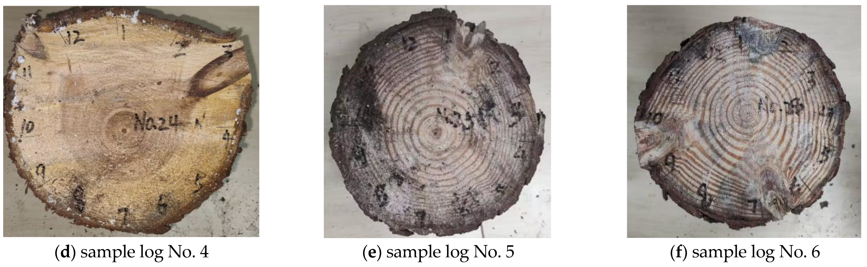
2.1. Testing Materials

Six logs, comprising four fir logs and two pine logs with natural knots, were sourced from the Xinxin Jinshun wood processing mill in Fujian province for this study. Each log was 200 cm in length, with a diameter at breast height (DBH) of approximately 28 cm. To facilitate the measurements, log samples with prominent and visible natural features were selected. A 60 cm section was cut from each log, and from this section, a log disc with a height of 30 cm was obtained. Each disc was then numbered for identification. The processing steps for the log samples used in this study are illustrated in Figure 1.

The cross sections of the natural knot side for the six test log samples are shown in Figure 2. Among these, sample logs No. 2, No. 3, and No. 5 have only one knot, sample logs No. 1 and No. 4 have two knots, and only test log No. 6 has three knots. The basic information regarding the tree species and cross-sections of the six sample logs used in this study is summarized in

Table 1. Basic information of log sample.

Sample log/No.	Diameter/cm	Number of Knots	Sample Log Shape	Species
1	28	2	Deviated from the positive circle	fir
2	26	1	Close to the round	fir
3	21	1	Close to the round	fir
4	23	2	Deviated from the positive circle	fir
5	20	1	Deviated from the positive circle	pine
6	23	3	Deviated from the positive circle	pine

.

2.2. Test Method

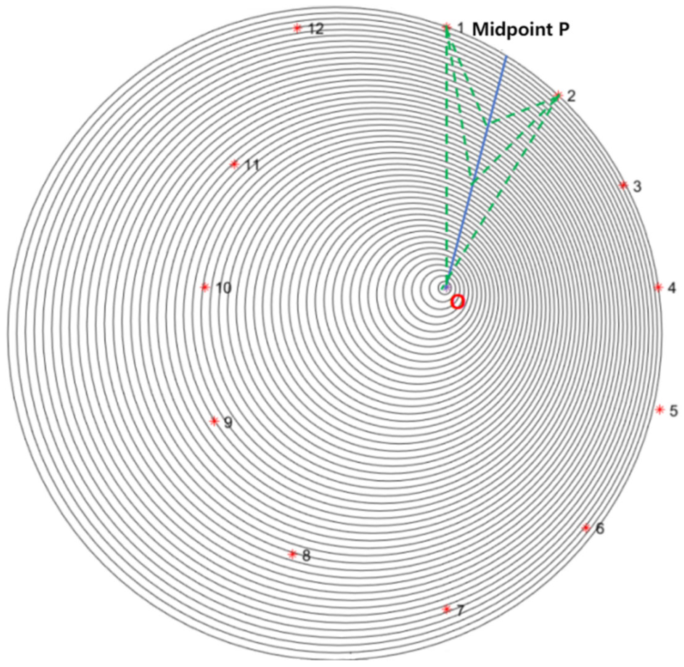
2.2.1. Measurement Method of Stress Wave in Cross Section of Test Log

A stress wave is a form of stress and strain interference propagation. In deformable solid media, mechanical disturbances manifest themselves as changes in the particle velocity and corresponding changes in the stress and strain states. The change in the state of stress and strain propagates in the form of a wave, which is known as a stress wave. The velocity of a stress wave is calculated as follows.

$$c=\sqrt{{\displaystyle \frac{E}{\rho }}}$$

(1)

where c is the stress wave propagation velocity, E is the dynamic elastic modulus of the material, and ρ is the density of the material.

The propagation speed of stress waves varies among different mesons, for example, the propagation speed in the air is about 340 m/s. The propagation speed in water is about 1480 m/s. The propagation speed in metals depends on the type and density of the metal, ranging from 5000 to 8000 m/s.

A Fakopp microsecond timer (produced by Fakopp in Sopron, Hungary), as shown on the right side of Figure 3, was used to measure the stress wave propagation within logs in this paper. First, a center point was identified on the cross-section of the sample log, and then 12 measurement points were determined along the outer circle of the sample log disk and sequentially marked, that is, a test measurement point was arranged every 30 degrees (as shown in Figure 3).

The transmitting and receiving ends of the microsecond meter were inserted into measurement points 1 and 2 on the log’s cross-section, respectively (as shown in Figure 3). The transmitting end was tapped three times consecutively, and the stable repeated value was recorded as the stress wave propagation time between measurement points 1 and 2. Subsequently, while keeping the transmitting end fixed, the receiving end was sequentially inserted into measurement points 3 through 12, repeating the measurement process to determine the stress wave propagation time between each pair of points from 2 to 12.

After completing the measurements for all the paths from measurement point 1, the transmitting sensor was moved to measurement point 2, and the process was repeated for measurement points 3 through 12. This procedure was continued until stress wave propagation times were recorded for all the combinations, resulting in a total of 66 data points (12 × 11/2) for each log. This entire measurement process was repeated for the cross-sections of six test logs to obtain comprehensive stress wave propagation time data.

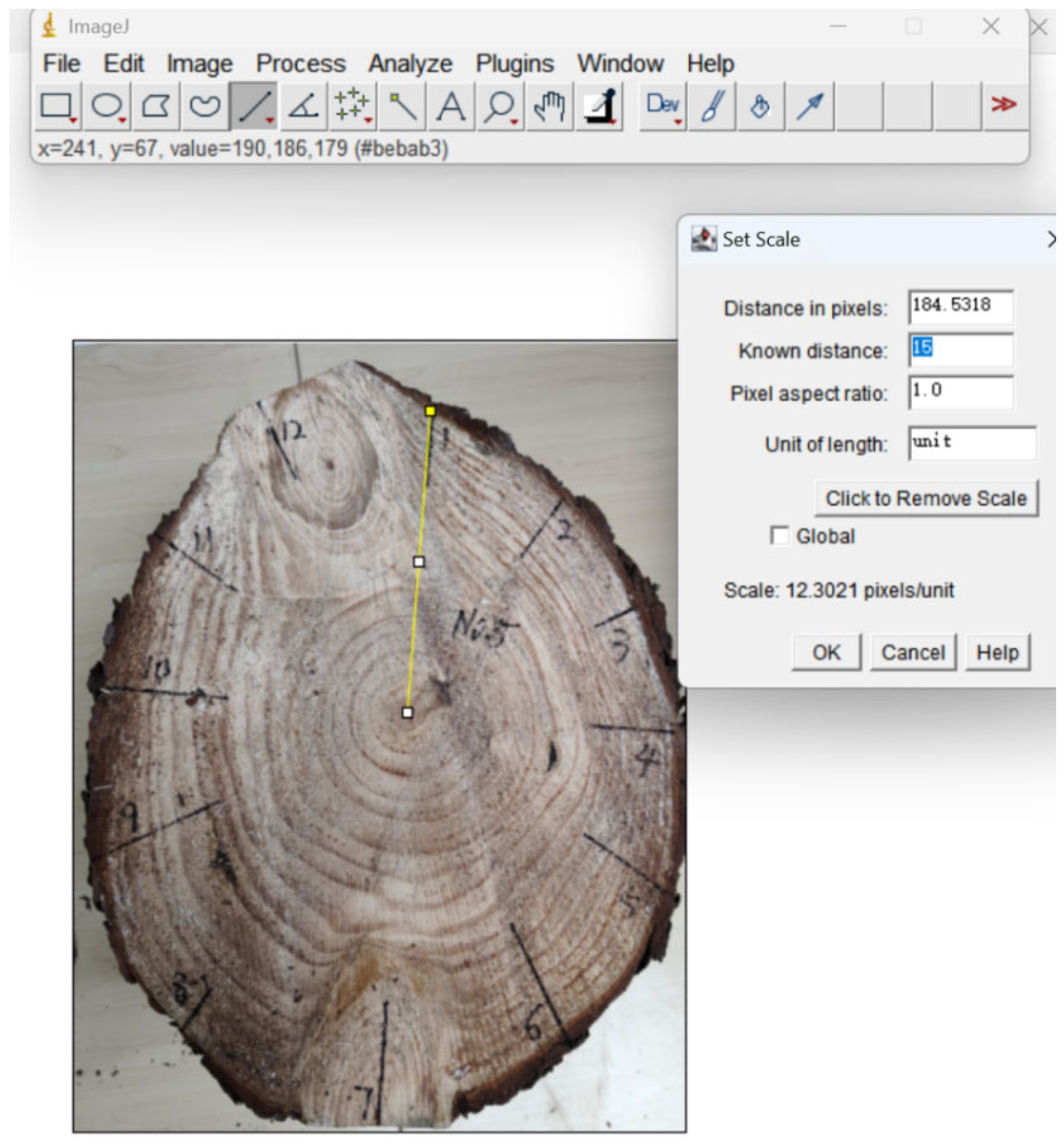
2.2.2. Calculation Method of Actual Area of Log Cross Section and Section

The cross-sectional area and knot area of the sample logs were estimated using image processing software v1.48. First, the radius, R, of each log’s cross-section was measured (as shown in Figure 4). Photographs were then taken of the cross-sections of the six sample logs. These images were imported into the image processing software, where the radius of each cross-section was marked using the ruler tool, and the measurement scale was set. The actual radius length of the log was then input into the software (as shown in Figure 4). The software calculated the cross-sectional area and the knot area based on the measured proportions.

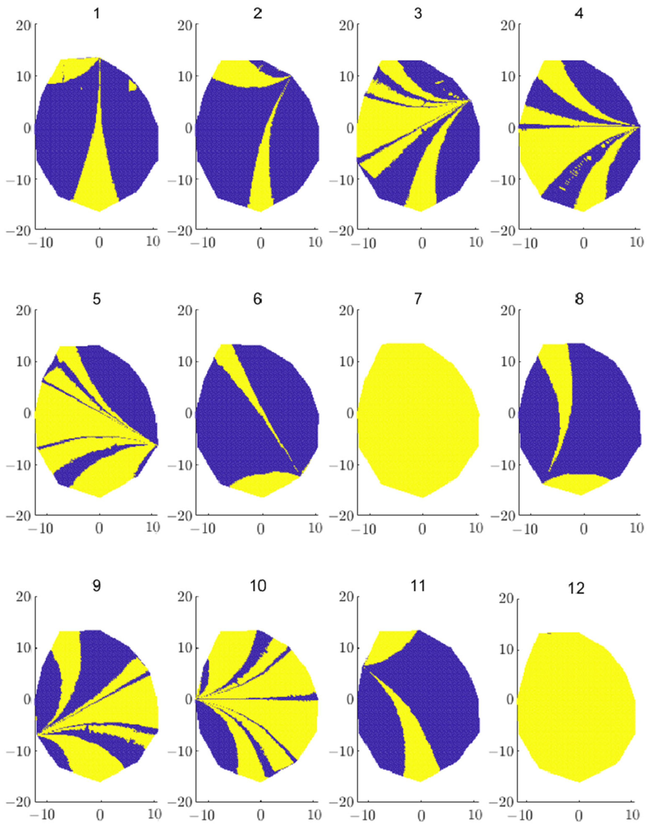
2.3. Algorithm Steps

(a)

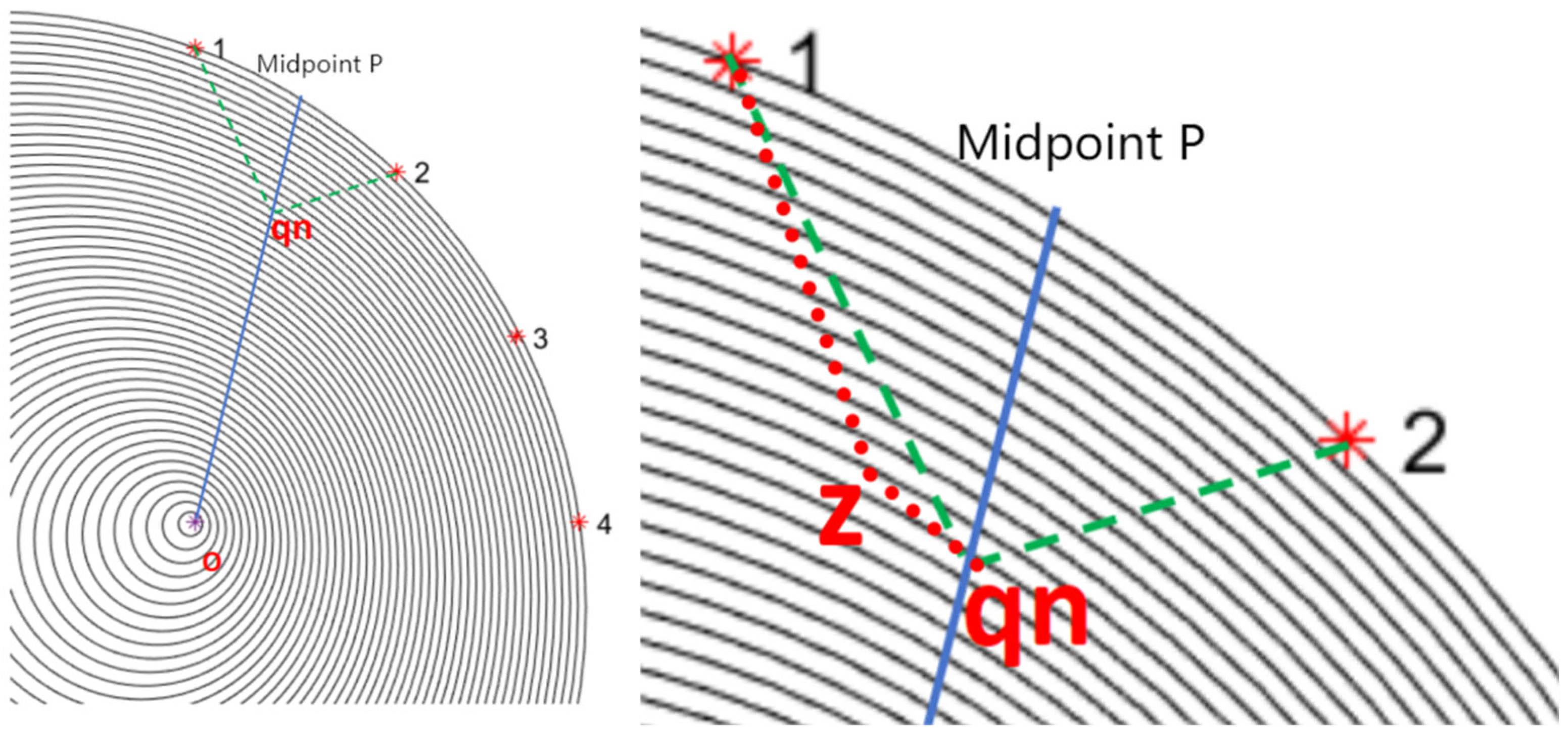
Method to eliminate the influence of the stress wave propagation time based on the external shape

It was found that the appearance and shape of the log cross-section significantly affect the propagation speed of stress waves, and the propagation path of the stress wave within the log cross-section is not necessarily a straight line. According to wave fluctuation theory, the propagation speed of stress waves in different media is influenced by the medium’s density and elastic modulus. In logs, the density varies between the pith, heartwood, and sapwood. Therefore, this study suggests that the shortest path for stress wave propagation between two points is not a straight line but a curve.

Under the ideal assumption of a circular log cross-section, the closer the propagation path is to a 90-degree angle relative to the log’s center, the faster the stress wave travels. Additionally, the closer the path is to the wood’s center, the higher the propagation speed. Since the exact internal stress wave speed distribution within the wood cannot be precisely determined, the study approximates this distribution by drawing a circle that passes through two points and their midpoint. By estimating the stress wave speed at each layer of the log, the shortest propagation time path across the log’s cross-section can be determined.

(b)

Find methods for the shortest propagation path under this model

In this study, an iterative method is employed to determine the shortest stress wave propagation path within the log cross-section. Initially, the fastest stress wave in the log is used, and a stress wave velocity curve is preset for each ring layer inside the cross-section (as shown in Figure 5).

The shortest propagation path is then calculated between the measurement points (as illustrated in Figure 6). The midpoint, OP, between these two points and the log’s centerline, are identified, and a connection is made between points 1 and 2. The stress wave propagation time along this line is then calculated to determine the shortest propagation time under these conditions (as shown in Figure 7).

The formula for calculating the shortest propagation time of the two-point-to-midline OP is as follows:

$${\mathrm{T}}_{\min 1}=\min \left[\left({\mathrm{L}}_{{\mathrm{p}}_{\mathrm{i}}{,\mathrm{q}}_{\mathrm{n}}}{+\mathrm{L}}_{{\mathrm{p}}_{\mathrm{j}}{,\mathrm{q}}_{\mathrm{n}}}\right)/\left({\displaystyle \sum _{\mathrm{x}=1}^{\mathrm{n}-1}{\mathrm{V}}_{\mathrm{x}}}\right)/\left(\mathrm{n}-1\right)\right]$$

(2)

where T_min1 is the shortest transmission time in the two-line segment case. p_i is one of the 12 measuring points in the wood periphery, and i is not equal to j. n is the number of circles through which the segment q_n is the intersection of the OP segment and any layer,${\mathrm{L}}_{{\mathrm{p}}_{\mathrm{j}},{\mathrm{q}}_{\mathrm{n}}}$ is the distance between two points, and V_x is the stress wave propagation speed in the x circle.

After determining the position of q_n, further determination of the propagation path of the stress wave is needed. Look for the shortest propagation time path from z to q_n and z to p_i at some point on the outward layer, and then determine the point z on the outward layer as the starting point. Next, find such points on each layer, and finally form the approximate path of the fastest stress wave propagation (as shown in Figure 8 and Figure 9).

The formula for optimizing the position of the propagation path in each layer is:

$${\mathrm{T}}_{\min 2}=\min \left[{\mathrm{L}}_{{\mathrm{p}}_{\mathrm{i}},\mathrm{z}}/\left({\displaystyle \sum _{\mathrm{x}=1}^{\mathrm{n}-2}{\mathrm{V}}_{\mathrm{x}}}\right){+\mathrm{L}}_{{\mathrm{z},\mathrm{q}}_{\mathrm{n}}}{/\mathrm{V}}_{\mathrm{n}-1}\right]$$

(3)

where T_min2 is the shortest transmission time in this case. p_i is one of the 12 points in the wood periphery, n is the number of circles through which the segment passes, ${\mathrm{L}}_{{\mathrm{p}}_{\mathrm{i}},\mathrm{z}}$, ${\mathrm{L}}_{\mathrm{z},{\mathrm{q}}_{\mathrm{n}}}$ is the distance between two points, and V_x is the stress wave propagation speed in the x circle.

Using the preset stress wave velocity curve does not accurately reflect the stress wave velocity distribution within the log’s cross-section, so the curve must be adjusted iteratively.

Since the transmission path near the log’s periphery is the shortest, it is less affected by uncertainties than longer transmission paths. The algorithm begins with the outer wave velocity and iteratively updates the wave velocity curve. Paths that pass through a similar number of layers are selected, and their propagation times are compared with experimental data. If the propagation time near the outer layer closely matches the experimental data, the stress wave velocity curve for that section is determined. If the times do not match, the wave speed is adjusted (either increased or decreased). If multiple adjustments fail to meet the requirements, the path with the largest discrepancy from the experimental data is eliminated. The remaining data are then used to further adjust the wave velocity curve until the algorithm’s calculated time aligns with the data. Once the stress wave velocity for this section is determined, the velocity curve for other parts of the log is adjusted accordingly until the process is complete (as shown in Figure 10). Finally, the percentage difference between the algorithm’s calculated propagation time and the experimental data is analyzed (as shown in

Table 2. The percentage difference between the propagation time obtained by the algorithm and the experimental data time.

	1	2	3	4	5	6	7	8	9	10	11	12
1	0	0.48	7.63	4.89	2.66	1.02	−17.68	−5.38	−1.66	−8.85	−8.53	−20.08
2	0	0	3.04	−0.88	3.39	3.07	−12.84	1.98	3.38	−0.20	−1.83	−19.17
3	0	0	0	5.10	5.54	3.93	−13.90	−1.15	4.07	−260.35	1.17	−15.19
4	0	0	0	0	3.13	−0.17	−17.18	−3.99	−199.46	3.13	0.86	−15.76
5	0	0	0	0	0	−5.17	−22.95	−6.89	0.41	−392.81	4.42	−13.66
6	0	0	0	0	0	0	−23.33	−8.61	−7.04	−3.91	−2.64	−11.77
7	0	0	0	0	0	0	0	−19.58	−16.27	−14.30	−15.16	−34.96
8	0	0	0	0	0	0	0	0	−3.31	−3.51	1.80	−13.42
9	0	0	0	0	0	0	0	0	0	−3.16	−1.24	−14.75
10	0	0	0	0	0	0	0	0	0	0	−3.42	−19.08
11	0	0	0	0	0	0	0	0	0	0	0	−39.03
12	0	0	0	0	0	0	0	0	0	0	0	0

). If the error exceeds 10%, it is determined that a knot is present in the propagation path (as shown in Figure 11).

(c)

Log cross-section tomographic imaging method based on the shortest path method

After obtaining the appropriate stress wave velocity curve, the curve for the remaining sections between each measurement point is completed through interpolation. Next, the direction of the knot is determined from each measurement point (as shown in Figure 12). In Figure 12, the yellow part represents the direction of the knot, starting from each point, and the blue part represents the direction from each point, where there is no knot. By superimposing the defect images from all 12 measurement points, a composite defect image is created. Areas with greater overlap in the image indicate a higher likelihood of the presence of a knot.

3. Results and Discussion

3.1. Results and Analysis of Stress Wave Tomography of Cross Section of Sample Logs

Using an iterative stress wave wood imaging algorithm based on the log’s appearance and the shortest propagation path method, the imaging results are presented in Figure 13, Figure 14 and Figure 15. To effectively visualize the tomography, a three-color scheme is applied to represent the measurement results of the sample log’s cross-section. In this scheme, areas closer to yellow indicate regions where the stress wave propagation velocity deviates significantly from the norm, while areas closer to blue indicate regions where the propagation speed closely aligns with the expected wave velocity. The green areas represent an intermediate state, where the stress wave propagation speed is between the extremes. In summary, blue indicates healthy areas of the cross-section, green represents regions with potential defects or deviations in the stress wave velocity, and yellow highlights areas where knots are likely located.

(a)

Single-knot sample log

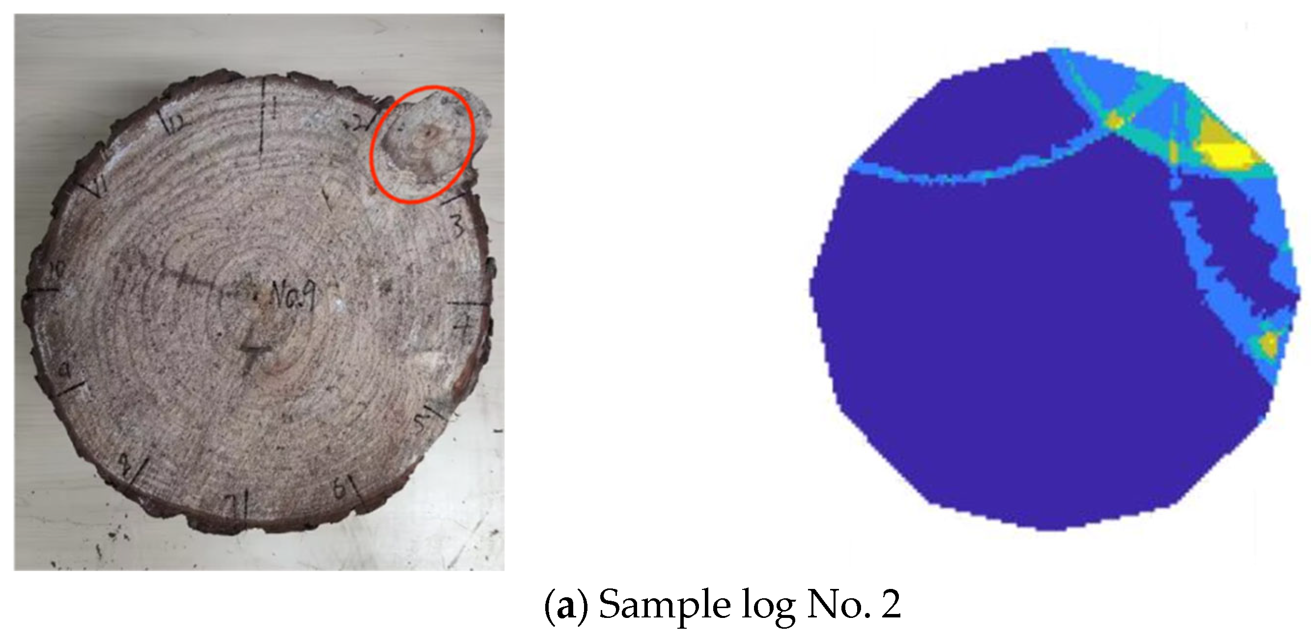
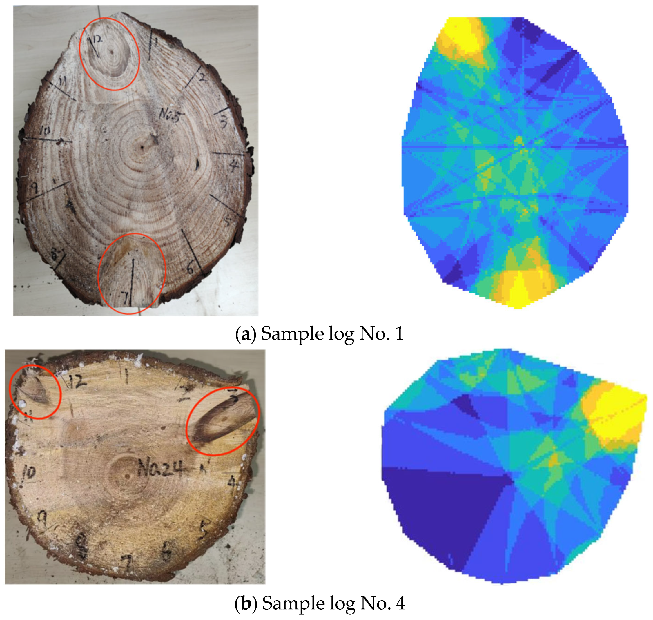
The imaging results for the single-knot sample logs (No. 2, No. 3, and No. 5) are shown in Figure 13. For sample log No. 2, the actual knot is located in the upper right of the cross-section, specifically between measurement points 2 and 3. The imaging results show an obvious yellow area between these points, which corresponds well with the actual knot position. For sample log No. 3, the actual knot is on the right side of the cross-section, between measurement points 2 and 4. The imaging algorithm predicts the knot’s location roughly between measurement points 2 and 3, and this prediction is fairly accurate. In the case of sample log No. 5, the actual knot is located above the cross-section, between measurement points 1 and 2. The imaging algorithm identifies two areas with an abnormally high stress wave velocity on the cross-section: one between measurement points 12 and 2, which aligns well with the actual knot position, and another between measurement points 10 and 12. However, there is no knot in this second area, suggesting that the abnormal yellow region may be due to system errors, data point anomalies, or the absence of log bark in this measurement area. Additionally, Figure 13 shows that the shape and size of the knots determined by the tomography algorithm differ somewhat from the actual knot sizes in sample logs No. 2, No. 3, and No. 5.

Therefore, for the single-knot sample log, the tomographic imaging algorithm proposed in this paper can roughly predict the location of the knot within the log’s cross-section. However, it cannot accurately predict the shape and size of the knot, and there are noticeable differences compared to the actual knot. Additionally, it should be noted that the imaging algorithm may sometimes predict a single-knot log as having two knots, which requires further analysis and judgment.

(b)

Double-knot sample log

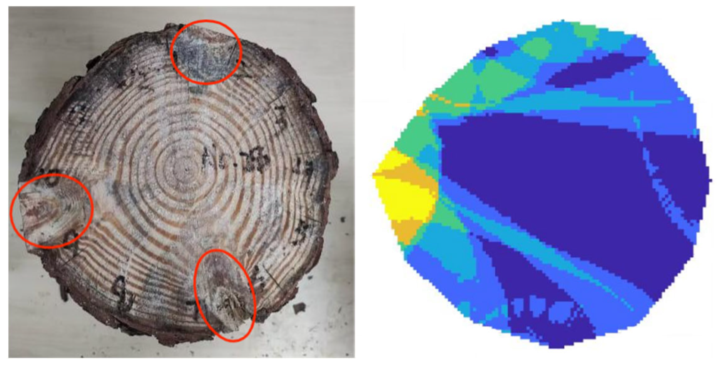
The imaging results for the double-knot sample logs (i.e., logs No. 1 and No. 4) are shown in Figure 14. For sample log 1, the actual knots are located near measurement points 12 and 7, and the imaging algorithm accurately predicts these locations, with the yellow areas corresponding to these points. For sample log 4, the two actual knots are located in the upper left and upper right of the cross-section, specifically between measurement points 11 and 12, and between measurement points 2 and 4. The imaging algorithm, however, identifies only one area with significant stress wave velocity anomalies, located between measurement points 2 and 4. This prediction matches the actual location of the right-side knot, but the algorithm fails to predict the knot in the upper left corner of the cross-section, as no significant yellow area or wave speed anomaly is detected in that region. Additionally, Figure 14 shows that, for the double-knot sample logs, the shape and size of the knots predicted by the tomographic imaging algorithm still differ from the actual knots, consistent with the observations for the single-knot sample logs.

Therefore, for the double-section sample log, the approximate location of the log can still be roughly predicted through the cross-section, but the shape and size of the knot cannot be very accurately predicted, and there are some differences between the shape and size of the actual knot. At the same time, it should also be noted that the imaging algorithm may judge the double-knot log as a single-knot log, that is, the actual knot log may be missed in the log, and further analysis and judgment are needed.

(c)

Three-knot sample logs

The imaging results for the three-section sample logs (No. 6) are illustrated in Figure 15. For this sample log, the three actual sections are situated between points 1 and 2, 6 and 7, and 9 and 10. Notably, the cross-section reveals a single prominent yellow area between measuring points 9 and 10, which corresponds to the actual location of one of the sections. Additionally, for the knots between measurement points 1 and 2 and between points 6 and 7, the imaging algorithm identifies these regions. However, due to the subtle nature of the abnormal fluctuations, their presence cannot be conclusively determined by fault imaging alone. Figure 15 also indicates discrepancies in the shape and size of the knots detected by the algorithm compared to their actual dimensions.

Therefore, while the tomographic imaging algorithm can approximate the locations of some knots in the three-section sample log, it cannot accurately predict the complete position of all the knots in the cross-section. The algorithm’s predictions of knot shapes and sizes are also imprecise, with noticeable differences from the actual knots. For sample logs with three or more knots, it is crucial to scrutinize areas of abnormal wave velocity identified by the imaging algorithm, as these may indicate knot locations, and verify the presence of multiple knots within the log.

3.2. Analysis of Prediction Results of Sample

Although the tomographic imaging results of the sample log (e.g., Figure 13, Figure 14 and Figure 15) demonstrate the predictive capability of the shortest propagation path algorithm in determining the position, shape, and size of knots, the accuracy and precision of the proposed algorithm in relation to the relative error between the measured areas of the six sample logs still need to be evaluated.

Table 3. Sample knot detection results.

Number of Sample	Actual Measured Cross-Sectional Area/cm2	Actual Measured Knot Area/cm2	The Area Calculated by the Algorithm/cm2	Relative Error/%
1	639.945	72.326	60.479	16.38
2	590.761	22.202	18.199	18.29
3	328.242	15.520	11.711	24.54
4	441.630	36.669	25.342	30.88
5	332.706	14.142	16.357	15.66
6	400.037	37.801	18.111	52.08

presents the measured knot areas for sample logs No. 1 through No. 6, along with the calculated knot areas and corresponding error calculations. From Table 3, the smallest relative error (Dt) between the predicted knot area and the actual knot area for sample log No. 1 is 15.66%, while the largest relative error is 52.06% for sample log 6. The relative error (Dt) for the knot areas calculated by the algorithm ranges from 15.66% to 52.08%. Table 3 also reveals that with the exception of sample log 6, the relative errors for the other sample logs are generally within 31%. Notably, sample logs No. 1, No. 2, and No. 5 exhibit relative errors of less than 20%, indicating that the proposed algorithm can reliably predict the knot area size in the sample logs. Additionally, when considering the imaging results shown in Figure 13, Figure 14 and Figure 15, the algorithm’s predicted knot areas are generally smaller than the measured areas. This discrepancy is likely due to some missed or misjudged cases. Despite this, the algorithm accurately predicts the knot positions. The smaller predicted knot areas may result from the algorithm not accounting for areas near the log’s internal knots or from the difficulty in distinguishing between stress wave velocities in areas with and without knots.

Additionally, when analyzing the cross-sectional appearance of each sample log, sample logs No. 2, No. 3, and No. 5 exhibit a shape close to a perfect circle, with only one knot visible on the cross-section. Among these, the tomography algorithm performed best on sample log No. 2 (see Figure 13a), showing minimal interference in the imaging results. The algorithm effectively identified a small knot in the lower right corner of the cross-section, represented by a minor, distinct yellow area. For sample log No. 3, the knot area predicted by the imaging algorithm is smaller than the actual knot area. This discrepancy arises because the stress wave propagation path for log No. 3 between measurement point 4 bypasses the knot’s location on the cross-section, so the stress wave velocity is unaffected. As a result, the algorithm cannot detect the knot along the path between measurement points 2 and 4, leading to an underestimation of the knot area in the final imaging. Lastly, for sample log No. 5, despite the relative error of the knot area being less than 20%, the imaging results contain interfering color blocks (see Figure 13c). This issue may be attributed to bark detachment at measurement point 3, which likely affected the imaging accuracy.

For sample logs No. 1, No. 4, and No. 6, the cross-sectional wood shapes deviate from a perfect circle, with sample logs No. 1 and No. 4 each containing two knots, and sample log No. 6 containing three knots. Sample log No. 1 shows a good fault imaging effect, accurately predicting the area, shape, and position of the knots. In contrast, for sample log No. 4, the relative error of the knot area reaches 30.88%. This discrepancy may be due to some measurement points being located in the wood, which introduces deviations in the propagation path and results in errors in the final prediction. For sample log No. 6, the imaging algorithm successfully predicts the position and shape of only one knot, while the other two knots are only visible in the propagation path but not predicted accurately. This limitation results in a relative error of over 50% for the knot area. The presence of multiple knots in the section may have caused gaps in the data, preventing the algorithm from detecting all the knots accurately and leading to imaging errors.

In summary, the proposed algorithm demonstrates good performance in predicting faults within logs with cross-sectional shapes close to a circle. However, its accuracy diminishes for logs with significant deviations from a circular shape and small faults. Further experimental research and algorithm improvements are needed to enhance fault imaging and prediction accuracy for these cases.

4. Conclusions

This paper proposes an algorithm for stress wave log knot fault imaging based on log shape appearance. The algorithm involves designing the stress wave velocity distribution for log faults, finding the fastest stress wave propagation path and using data comparison and iterative methods to determine the optimal stress wave velocity distribution. Finally, tomographic imaging results are obtained through image superposition. The conclusions are as follows:

(1)

The tomographic imaging algorithm proposed can roughly predict the knot locations in logs with one, two, or three knots. However, it is less accurate in predicting the shape and size of the knots, with some discrepancies between the predicted and actual dimensions. Additionally, the algorithm might misidentify a single-knot log as having two knots or a double-knot log as having one knot, potentially missing actual knots. For logs with three or more knots, the algorithm relies on single log data without artificial data screening, which may lead to the incomplete detection of knots due to a lack of normal propagation time data. Therefore, it is important to verify the presence of multiple knots inside the log.

(2)

The relative error between the knot area calculated by the algorithm and the measured knot area ranges from 15.66% to 52.08%. Except for sample log No. 6, the relative errors for the other sample logs are generally within 31%, with sample logs No. 1, No. 2, and No. 5 showing relative errors of less than 20%. Although there are some discrepancies, the algorithm provides a rough estimate of the knot area. Further improvements are needed to enhance the prediction accuracy of the knot area.

(3)

The algorithm performs well for logs with cross-sectional shapes close to an ideal circle and can provide accurate tomographic imaging and prediction. However, it struggles with logs that have significant deviations from a circular shape or very small faults. The imaging effect and prediction accuracy decrease under these conditions. Further experimental research and algorithm refinement are necessary to improve fault imaging and prediction accuracy for such cases. There are few studies on the detection algorithm of stress wave wood NDT. This paper provides an algorithm for detecting detection, which provides a little basis for subsequent algorithm research.

References

1. Cui, H.O.; Liu, M. Study on resource dynamics in the ninth Forest Resources Inventory in China. West. For. Sci. 2020, 49, 90–95. [Google Scholar]
2. Yu, C. The Current situation and management suggestions of forest quality in China. For. Econ. China 2020, 6, 91–94. [Google Scholar] [CrossRef]
3. Broda, M.; Mazela, B.; Królikowska-Pataraja, K.; Hill, C.A. The use of FT-IR and computed tomography non-destructive technique for water logged wood characterisation. Wood Res. 2015, 60, 707–722. [Google Scholar]
4. Wang, X.C. Study on Adhesive Shear Properties of Carbonized Bamboo/Larch Gum. Master’s Thesis, Central South University of Forestry and Technology, Changsha, China, 2021. [Google Scholar] [CrossRef]
5. FUJIMORI, T. Dynamics of crown structure and stem growth based on knot analysis of a hinoki cypress. For. Ecol. Manag. 1993, 56, 57–68. [Google Scholar] [CrossRef]
6. Yong, C.Z.; Li, Y.L. Physical and mechanical properties and utilization of Chinese wood. Guizhou For. Sci. Technol. 1991, 19, 69–70. [Google Scholar]
7. Wang, Y.R.; Zhao, R.J.; Jiang, Z.H.; Xu, Z.Y. Density analysis of the trunk, knots and branches of loblolly pine. For. Prod. Ind. 2016, 43, 14–17. [Google Scholar]
8. Hein, S. Knot attributes and occlusion of naturally pruned branches of Fagus sylvatica. For. Ecol. Manag. 2008, 256, 2046–2057. [Google Scholar] [CrossRef]
9. Newton, M.; Lachenbruch, B.; Robbins, J.M.; Cole, E.C. Branch diameter and longevity linked to plantation spacing and rectangularity in young Douglas-fir. For. Ecol. Manag. 2012, 26, 75–82. [Google Scholar] [CrossRef]
10. Björklund, L.; Moberg, L. Modelling the inter-tree variation of knot properties for Pinus sylvestris in Sweden. Stud. For. Suec. 1999, 14, 376–384. [Google Scholar]
11. Duchateau, E.; Longuetaud, F.; Mothe, F.; Ung, C.; Auty, D.; Achim, A. Modelling knot morphology as a function of external tree and branch attributes. Can. J. For. Res. 2012, 43, 266–277. [Google Scholar] [CrossRef]
12. Mäkinen, H.; Ojansuu, R.; Sairanen, P.; Yli-Kojola, H. Predicting branch characteristics of Norway spruce (Picea abies (L.) Karst.) from simple stand and tree measurements. Forestry 2003, 76, 525–536. [Google Scholar]
13. Jia, W.W.; Feng, W.J.; Li, F.R. Study on the number of lost rings in changbai larch plantation based on the node seed dissection data. J. Beijing For. Univ. 2020, 42, 87–98. [Google Scholar]
14. Chen, D.S.; Li, F.R.; Sun, X.M.; Jia, W.W. Headnut size prediction model of the larch plantation based on a linear mixed model. For. Sci. 2011, 47, 121–128. [Google Scholar]
15. Guan, Z.Z.; Lu, Q.F.; He, S.Y.; Qiu, Q.; Ma, W.J. Spatial distribution characteristics of the trunk nodes and their area prediction model. J. Cent. South Univ. For. Technol. 2021, 41, 20–28. [Google Scholar]
16. Jia, W.W.; Cui, C.; Li, F.R. Artificial Korean pine knot attributes based on a mixed effect model. J. Appl. Ecol. 2018, 29, 33–43. [Google Scholar]
17. Zhang, Z.C.; Li, F.R.; Chen, D.S. Study on the number of rings at different growth stages in larch plantation. Plant Res. 2010, 30, 320–324. [Google Scholar]
18. Hao, J.; Meng, M.J.; Huang, D.W.; Wei, J.L.; Li, Z.G.; Tang, J.X.; Xu, D.P. Distribution characteristics and prediction model of grid plantation. J. Nanjing For. Univ. (Nat. Sci. Ed.) 2017, 41, 100–104. [Google Scholar]
19. Gilbert, G.S.; Ballesteros, J.O.; Barrios-Rodriguez, C.A.; Bonadies, E.F.; Cedeño-Sánchez, M.L.; Fossatti-Caballero, N.J.; Trejos-Rodríguez, M.M.; Pérez-Suñiga, J.M.; Holub-Young, K.S.; Henn, L.A.W.; et al. Use of sonic tomography to detect and quantify wood decay in living tress. Appl. Plant Sci. 2016, 4, 60–72. [Google Scholar] [CrossRef]
20. Espinosa, L.; Arciniegas, A.; Cortes, Y.; Prieto, F.; Brancheriau, L. Automatic segmentation of acoustic tomography images for the measurement of wood decay. Wood Sci. Technol. 2017, 51, 69–84. [Google Scholar] [CrossRef]
21. Ladislav, R.; Martin, H. The type and degree of decay in spruce wood analyzed by the ultrasonic method in three anatomical direction. BioResources 2011, 6, 4953–4968. [Google Scholar]
22. Maurer, H.; Schubert, S.I.; Bächle, F.; Clauss, S.; Gsell, D.; Dual, J.; Niemz, P. A simple anisotropy correction procedure for acoustic wood tomography. Holzforschung 2006, 60, 567–573. [Google Scholar] [CrossRef]
23. Divos, F.; Divos, P. Resolution of stress wave based acoustic tomography. In Proceedings of the 14th International Symposium on Nondestructive Testing of Wood, Eberswalde, Germany, 2–4 May 2005; pp. 309–314. [Google Scholar]
24. Liu, J.X.; Gao, J.Q.; Li, C. Wood-defect image reconstruction using the LandWeber algorithm. J. Northeast For. Univ. 2019, 47, 125–128. [Google Scholar]
25. Yan, Z. Preliminary Study Based on 2D Image Reconstruction of Internal Defects; Northeast Forestry University: Harbin, China, 2007. [Google Scholar]
26. Liu, L.J.; Xie, Z.H.; Yang, C. Ray tracing algorithm based on boundary linear walk interpolation. J. South China Univ. Technol. (Nat. Sci. Ed.) 2014, 42, 23–28+35. [Google Scholar]
27. Cai, Y.L. Based on Shortest Path Ray Tracing; Northeast Forestry University: Harbin, China, 2015. [Google Scholar]
28. Wu, T. Study of Wood Defect Fault Reconstruction Based on Cell Back Projection; Northeast Forestry University: Harbin, China, 2016. [Google Scholar]
Figure 1. Schematic diagram of processing raw wood samples for experimental measurement.
Forests 15 01748 g001
Figure 2. Cross-section images of sample log.
Forests 15 01748 g002aForests 15 01748 g002b
Figure 3. Schematic diagram of operation method and experimental equipment.
Forests 15 01748 g003
Figure 4. Software operation method.
Forests 15 01748 g004
Figure 5. Preset wave velocity curve.
Forests 15 01748 g005
Figure 6. Sample 1.
Forests 15 01748 g006
Figure 7. Algorithm Process 1.
Forests 15 01748 g007
Figure 8. Algorithm Process 2.
Forests 15 01748 g008
Figure 9. Stress wave propagation path.
Forests 15 01748 g009
Figure 10. Adjusted stress wave velocity curve.
Forests 15 01748 g010
Figure 11. The stress wave propagation path after adjustment, with the red path indicating the presence of knots.
Forests 15 01748 g011
Figure 12. The defect image generated by each measurement point is the direction of the knot from this position: the units for the coordinate axis are centimeters.
Forests 15 01748 g012
Figure 13. Experimental samples No.2, No,3, No.5 and their imaging effects.
Forests 15 01748 g013aForests 15 01748 g013b
Figure 14. Experimental samples No.1, No.4 and their imaging effects.
Forests 15 01748 g014
Figure 15. Experimental sample No. 6 and its imaging effects.
Forests 15 01748 g015