Research on Non-Destructive Testing of Log Knot Resistance Based on Improved Inverse-Distance-Weighted Interpolation Algorithm

Abstract

The objective of this paper is to propose a non-destructive resistance detection imaging algorithm for log knots based on improved inverse-distance-weighted interpolation algorithm, i.e., the eccentric circle-based inverse-distance-weighted (ECIDW) method, to predict the size, shape, and position of internal knots of logs; evaluate its precision and accuracy; and both lay a theoretical foundation and provide a scientific basis for predicting and assessing knots in standing trees. Six sample logs with natural knots were selected for this study. Resistance measurements were performed on the log cross-sections using a digital bridge, and resistance tomography was conducted using the improved ECIDW algorithm, which combines the azimuth search method with the eccentric circle search method. The results indicated that both the conventional inverse-distance-weighted (IDW) algorithm and the ECIDW algorithm accurately predicted the positions of the knots. However, neither algorithm was able to predict the shape of the knots with high precision, leading to some discrepancies between the predicted and actual knot shapes. The relative error ($D{t}_1$) between the knot areas measured by the IDW algorithm and the actual knot areas ranged from 18.97% to 88.34%. The relative error ($D{t}_2$) for the knot areas predicted by the ECIDW algorithm ranged from 1.82% to 74.16%. The average prediction accuracy for the knot areas using the IDW algorithm was 51.58%, compared to 72.90% using the ECIDW algorithm. This indicates that the ECIDW algorithm has higher accuracy in predicting knot areas compared to the conventional IDW algorithm. The ECIDW algorithm proposed in this paper provides a more reasonable and accurate prediction and evaluation of knots inside logs. Compared to the conventional IDW algorithm, the ECIDW algorithm demonstrates greater precision and accuracy in predicting the shape and size of knots. While the resistance method shows significant potential for predicting internal knots in logs and standing trees, further improvements to the algorithm were needed to enhance the imaging effects and the precision and accuracy of knot area and shape predictions.

1. Introduction

Wood is a biomass material that, during its growth, is susceptible to the invasion of harmful organisms, leading to defects such as decay, hollows, and knots. These defects result in a decline in the wood’s mechanical properties and reduced utilization rates [1]. To avoid damaging the wood, non-destructive testing (NDT) technology is employed to quickly and accurately detect these defects. This technology not only provides a scientific basis for standing trees evaluation and forest management but also serves as an important reference for optimizing timber processing. Knots are a common wood defect that affects both the strength and appearance of wood products, and they complicate processing. The size and number of knots are key indicators in determining wood grade during grading tests [2]. Knot detection has evolved from destructive methods and manual visual inspections to advanced non-destructive and automated techniques. As technology advances, knot detection methods continue to improve, enabling the early assessment of knot quantity, size, and distribution within logs. This helps enhance timber production, improve product quality, and increase yield. It also aids in establishing models to describe the patterns of knots more accurately [3]. Currently, most domestic research on the non-destructive testing of log knots focuses on surface detection and localization. There is limited research on the detection of internal knots within logs, making it crucial to further investigate this area.

In the non-destructive testing of internal knots in logs, there are currently very few methods available. One of the most studied and implemented techniques is CT inspection, specifically computerized X-ray tomography. This method works by scanning the target layer by layer using a precise X-ray beam and a highly sensitive detector. The data collected from these scans are processed by a computer to generate high-resolution images of the internal cross-sections, allowing for detailed insights into the condition of the desired parts. When applied to log inspection, the differences in X-ray absorption and transmission rates between knots and normal wood can reveal extensive information about the distribution and structure of knots within the log. This information can be used to derive parameters describing the knots, construct a model of the internal knots, and optimize the logging process accordingly [4,5]. However, this method has several drawbacks, including the presence of radiation, which poses health risks, as well as its high cost. While it is relatively easy to observe and measure external knots using simple equipment, detecting internal knots requires more advanced tools. In addition, some researchers are exploring the possibility of predicting the performance parameters of knots without the need for sophisticated equipment, relying instead on other factors. Thomas developed a series of quantitative models to establish relationships between the external and internal defect characteristics of American boxwood logs. By using visible external features, they aimed to predict internal knot characteristics. The results indicated that for most knots, the prediction error was small and the correlation was strong, particularly for size-related predictions. However, the correlation was weaker for more complex defects such as occasional bulging, clustering, and twisting or distortion [6].

In recent years, non-destructive testing technology has gained widespread application in the wood industry, with the resistance method emerging as a prominent technique due to its portability, ease of operation, and accessibility of relevant instruments and equipment [7]. This method is particularly advantageous in detecting wood defects, offering easier acquisition of defect information compared to other methods. As a result, it has become widely adopted in the field of non-destructive wood testing [8]. The basic principle of electrical resistance tomography (ERT) involves measuring the distribution of resistance across a wood cross-section and visualizing the data obtained. The resulting image displays the resistance levels of different areas within the cross-section at the same height of the tree, allowing for detailed analysis of the wood’s internal structure. Extensive research on resistance tomography has been conducted both domestically and internationally. For instance, Just et al. were the first to apply data measured by geological exploration instruments, combined with corresponding mathematical algorithms, to timber inspection, introducing ERT technology to the field for the first time [9]. Weihs et al. conducted tests on beech trees using the ERT technique, demonstrating its capability to detect discoloration in the heartwood [10]. Similarly, Lin et al. performed resistance tomography imaging on three Asian plants, including Taiwan cedar, analyzing the resistance value patterns. They found that resistance tomography could effectively distinguish between heartwood and sapwood [11]. Bieker et al. [12] studied oak wood, focusing on the radial distribution of conductive material in the wood cross-section. They found that resistance changes were not related to moisture content and density but were influenced by the concentration of potassium and magnesium ions and the pH value at the boundary between sapwood and heartwood [12]. Ayodele used the four-probe method to test wood defects in living Acacia trees and simulated wood defects in a laboratory setting. The study revealed that the resistivity of defective positions in living Acacia trees was approximately four times higher than that of healthy positions [13]. Yue et al. [14] employed resistance tomography, stress wave, and micro-drilling resistance methods to quantitatively detect the degree of decay in living wood. The study concluded that the resistance method is more sensitive to early decay, while the stress wave method is more accurate when the decay is more advanced, and the impedance meter method is the most accurate in detecting different degrees of decay, particularly in severe cases [14]. Shi et al. used the micro-drill resistance method and electrical impedance tomography to quantify decay in red pine, finding that while the impedance meter could accurately measure decay in a one-dimensional direction, the ERT method was more effective in detecting decay in a two-dimensional cross-section [15]. These studies demonstrate the effectiveness of the resistance method in detecting wood decay. Moreover, there is a significant difference in resistance between the knotty and normal parts of the wood, with knots leading to a marked increase in resistance. This highlights the practical value of using the resistance method for detecting knots in wood.

The IDW algorithm was initially applied in meteorological and geological imaging studies. Liu Guangming et al. used the spectral index method and IDW method to analyze and evaluate the three-dimensional spatial variability of soil salinity, which improved the accuracy of regional soil salinity predictions [16]. Wang et al. applied the IDW method to obtain meteorological data in the Yangtze and Yellow River Basins, uncovering relationships between human activities and meteorological conditions [17]. Similarly, Chen et al. [18] analyzed the relationship between air temperature and altitude using both the IDW and Kriging methods. Their results indicated that the IDW model performed slightly better than the Kriging model in low-temperature environments [18]. The IDW algorithm is based on the spatial distribution law of unknown regions, yielding good experimental results. It is widely used in meteorological and geographic imaging due to its fast computation speed, broad applicability, and low storage requirements [19]. However, the standard IDW algorithm does not account for the common location of defects. When applied to resistance tomography imaging of wood knots, the following issues may arise: (1) the attribute values of interpolation points are influenced by all known points within a certain range, increasing the algorithm’s complexity; (2) the attribute values are also dependent on the distances between all known points within that range, without considering that most knots are located at the wood’s edge.

To address these issues, this study proposes an improved IDW interpolation algorithm, the ECIDW method, for resistance tomography imaging of log knots. Multiple sample logs were used for tomography using both the IDW and ECIDW methods, and the imaging results were compared to evaluate the effectiveness of the ECIDW algorithm.

2. Materials and Methods

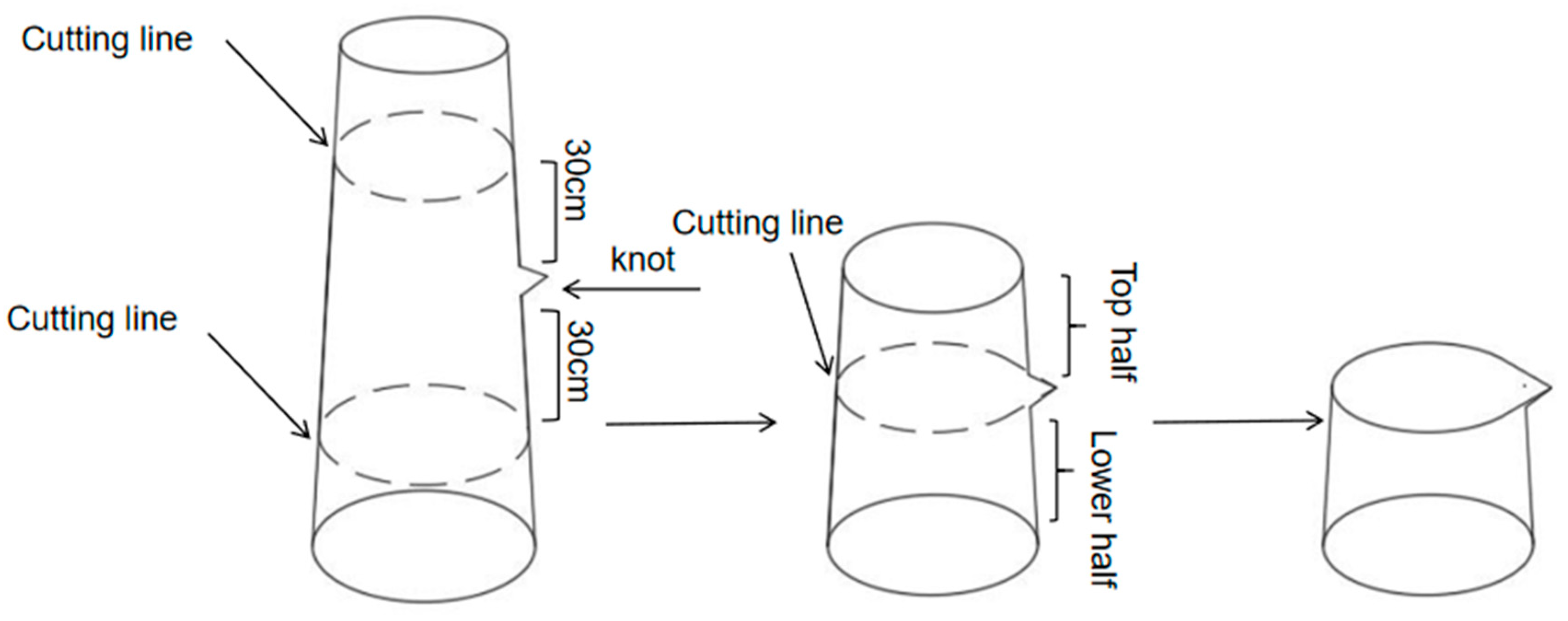
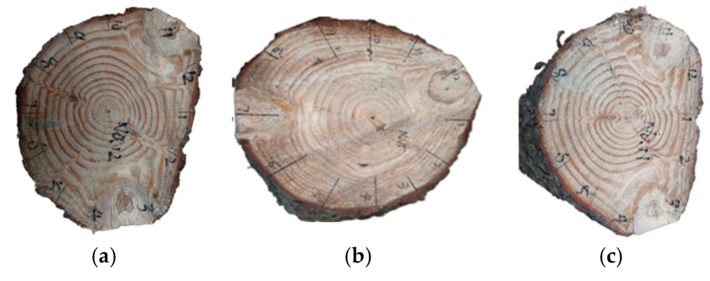
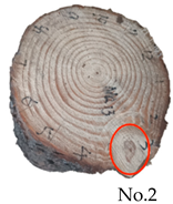
2.1. Test Material

The six test logs with natural knots used in this study were sourced from Fujian Xinxin Jinshun wood processing mill. The logs included five pine (Pinus) logs and one fir (Cunninghamia lanceolata (Lamb.) Hook.). Each log measured 200 cm in length with a diameter at breast height (DBH) of approximately 25 cm. To facilitate test measurements, prominent and large natural knots were selected from the surface of the logs. The selected knots were positioned so that the distance between the top and bottom of each knot was 30 cm. The logs were then cut into segments, each 60 cm in length, with the selected knots centered within these segments. Each 60 cm segment was further sawn into two log discs, each 30 cm in height, with the knots centered on the cutting plane. The lower half of the log disc, measuring 30 cm in height, was uniformly chosen as the test specimen for measurement. Each of these test specimens was labeled and numbered accordingly. A schematic diagram of the processing and preparation of the test measurement log specimens is provided in Figure 1.

The cross-sections of the six test log specimens with natural knots on one side are illustrated in Figure 2 and Figure 3. Among these, specimen logs 1, 2, and 3 are single-knot specimens, while specimen logs 4, 5, and 6 are double-knot specimens. The species of the six specimen logs used in this study, along with the basic information of their cross-sections, are summarized in

Table 1. Basic information of the test log sample.

Specimen Log Number/No.	Specimen Log Species	Specimen Log Radius/cm	Cross-Sectional Area of Specimen Logs/cm2	Specimen Log Knotty Area/cm2
1	pine	10.2	432.24	18.14
2	pine	10.3	419.35	26.49
3	fir	11.8	440.42	7.12
4	pine	10.2	396.73	34.80
5	pine	12.9	613.69	55.59
6	pine	10.4	312.57	29.24

.

The cross-sectional area of the specimen logs and the area of the knots, as listed in Table 1, were estimated using image processing software. The process began by measuring the actual radius R of the cross-sections of the six specimen logs with a straightedge. Next, photographs of the cross-sections were taken. These images were then imported into the image processing software. In the software, the radii of the cross-sections were marked using the ruler tool, which provided the pixel length of each specimen log’s radius (as shown in Figure 4a). The measurement scale was then set by inputting the actual radius length R, obtained from the physical measurements (as shown in Figure 4b). Finally, the software was used to select the cross-sectional area and the knot area of each specimen log, allowing for an estimation of these areas based on the established measurement scale.

2.2. Test Equipment

The resistance of the specimen logs was measured across the cross-section using a Tonghui TH2811D LCR digital bridge (produced by Changzhou Tonghui Electronics Co., Ltd., Changzhou, China). This instrument features a measurement accuracy of 0.2%, a test frequency range of 100 Hz to 10 kHz, and a signal source output impedance of 30 Ω and 100 Ω. In resistance mode, the digital bridge directly measures the resistance of the resistor to be measured. When the resistor to be measured is connected to the bridge circuit, the bridge will automatically generate an AC signal to flow through the resistor, measure the voltage and current of the resistor, and calculate its resistance.

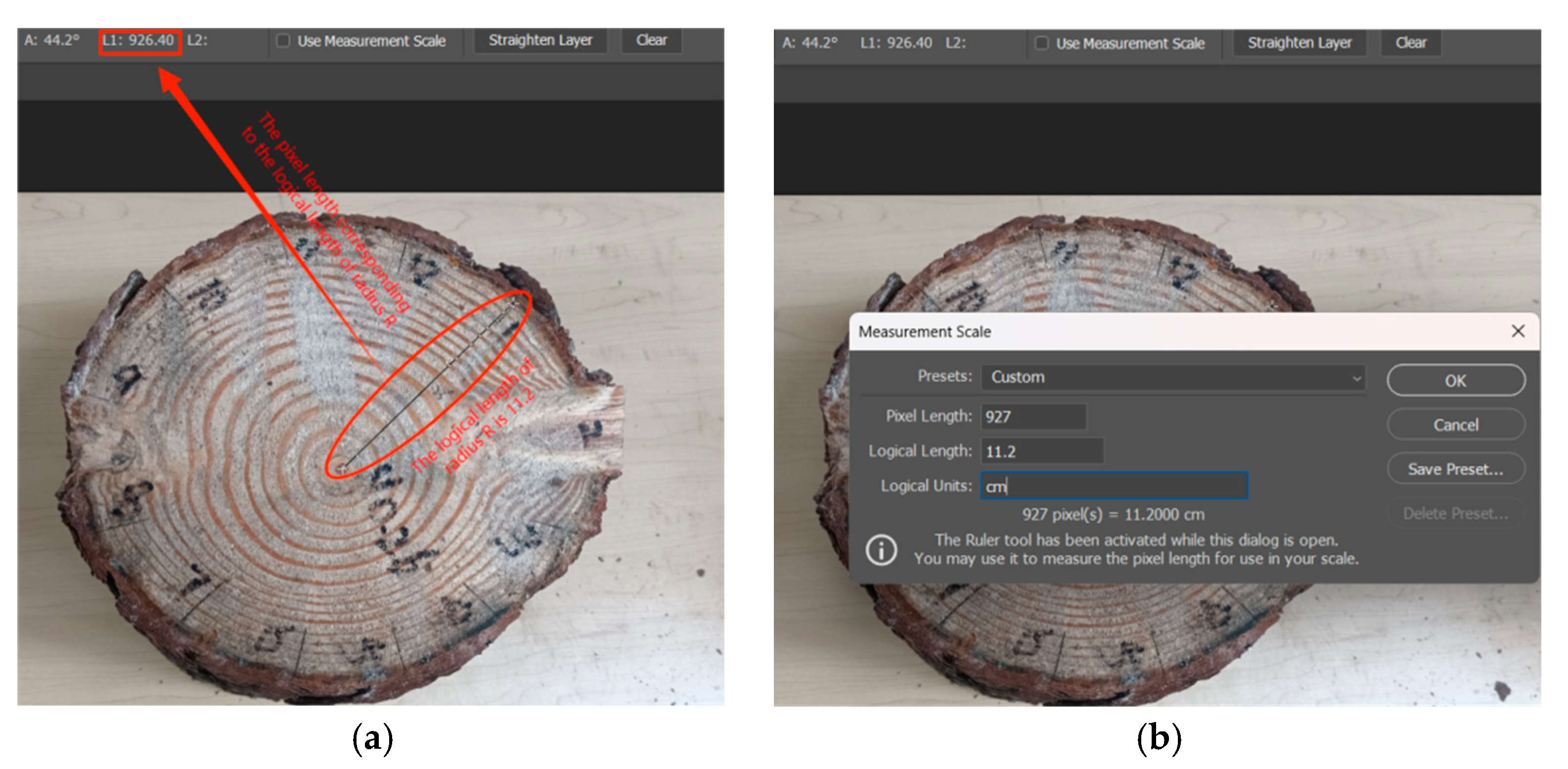
2.3. Test Methods

When measuring wood resistance, given the high resistance values of wood, the electrical impedance of the test object is modeled as a parallel combination of large resistance and small capacitance. The digital bridge is first turned on and allowed to warm up for 15 min. It is then zeroed for both open-circuit and short-circuit conditions. The digital bridge parameters are adjusted to the test resistance value, with the AC signal frequency set to 10 kHz, the signal level set to 1 V, the internal resistance set to 100 Ω, and the range set to automatic. Twelve resistance measurement points are uniformly selected around the circumference of the sample log. These points are marked on the cross-section of the log with a marker pen. Stainless steel nails are then arranged at these 12 measurement points and evenly spaced around the log disc, as shown in Figure 5. The nails are uniformly nailed into the log disc at the 12 designated measurement points.

After arranging the 12 stainless steel nails at the measurement points, the digital bridge electrode clamps are attached to the nails at measurement points 1 and 2 on the cross-section of the specimen log. Measurement is initiated, and the system is allowed to stabilize for approximately 30 s. The resistance value displayed is recorded, and the measurement is repeated three times to account for any systematic errors. The average resistance value is calculated and recorded as the path resistance from measurement point 1 to measurement point 2. This process is repeated for each pair of measurement points, recording the average resistance values for paths from measurement point 1 to all other points up to measurement point 12. The same procedure is followed for paths from measurement point 2 to measurement point 3, and so on, until all paths from measurement point 2 to measurement point 12 and measurement point 2 to measurement point 1 are covered. This results in a total of 12 × 12 resistance data matrices for the log cross-section. The measurements are then sequentially entered into the 12 × 12 resistance matrices. This procedure is repeated for each of the six specimen logs, resulting in complete resistance data sets for all tested cross-sections.

3. Improved Inverse-Distance-Weighted Interpolation Algorithm

3.1. Inverse-Distance-Weighted Interpolation Algorithm

Spatial interpolation is a method used to estimate the attributes of unknown points based on known point attributes. This method calculates the values for unknown points by analyzing the spatial relationships between known and unknown points. One commonly used spatial interpolation method is the IDW interpolation algorithm. The IDW method computes a weighted average of the attributes from known points within a specified distance range, with weights assigned based on the inverse of the distance between the interpolated point and the sample points. The closer a sample point is to the interpolated point, the greater its influence on the interpolated value [20]. Assume that the spatial prediction point is $p_i\left(xi,yi\right)\left(i=1, 2, 3, \cdots , n\right)$, and there are known points in its neighborhood $q_i\left(xi,yi\right)\left(i=1, 2, 3, \cdots , n\right)$, and $Z_{q_i}$ is the attribute value of the known points in the neighborhood. The attribute value of the point to be predicted $Z_{p_i}$ is calculated by the weighted average of the attribute value of the known point $q_i\left(xi,yi\right)$ in the neighborhood of the point to be predicted $Z_{q_i}$, and the size of the weight is related to the distance between the point to be interpolated and the point in the neighborhood, and $d_i$ is an interpolation method that is inversely proportional to the reciprocal of the distance [21], and its basic formula is as follows:

$$Z_{p_i}=\left[{\displaystyle \sum }_{i=1}^n{\displaystyle \frac{Z_{q_i}}{d_i^m}}\right]/{\displaystyle \sum }_{i=1}^n{\displaystyle \frac{1}{d_i^m}}$$

(1)

where $Z_{p_i}$ is the estimated value of the point to be predicted, $Z_{q_i}$ is the attribute value of the first known point in the neighborhood, $d_i$ is the distance between the first known point and the point to be predicted, and $n$ is the number of known points in the neighborhood involved in the interpolation computation. Indeed, $1/d_i^m$ is the weight coefficient, and the greater the $m$, the greater the influence of the known points nearer to the point to be predicted on the results of interpolation.

3.2. Inverse-Distance-Weighted Interpolation Algorithm Based on Eccentric Circle Search Method

This paper improved the IDW algorithm, and the new method was proposed as the ECIDW interpolation algorithm. This enhancement is designed for resistance tomography of log knots, aiming to generate accurate tomography images of the cross-sections of sample logs under test. The ECIDW algorithm introduces an optimization in the screening method used to select known points in the vicinity of predicted points. By combining the azimuthal search method with the distribution characteristics of the knots, the algorithm enhances the screening process. Known points are selected from an eccentric circle centered on the predicted point, allowing for a more precise calculation of the attribute values for the predicted points. This approach improves the accuracy of the tomography images by better aligning with the spatial characteristics and distribution patterns of the knots.

To perform spatial interpolation, the first step is to determine the attribute values of known nodes. For this, a right-angled coordinate system is established based on the cross-section of the sample log, and 12 measurement points are recorded. The resistance values along line segments connecting the two ends of the sample log are denoted as R_m∗n. The intersections of these line segments can be identified as multiple intersection points. As shown in Figure 6, point p is the intersection of line segments 1–8 and 4–12. Point p can have two different values, depending on three possible scenarios: (1) Both line segments 1–8 and 4–12 pass through the knot region, so their intersection point p also lies within the knot region. (2) If only one of the two line segments passes through the knot region, their intersection point p will not be within the knot region. (3) If neither line segment passes through the knot region, their intersection point p will not pass through the knot region either. Thus, only when both resistive segments pass through the knot region is the intersection point p likely to be in the knot region. Since the resistance in the knot region is higher than in the healthy part of the wood, the value of the segment with lower resistance is assigned to point p. Therefore, when there are multiple choices for the resistance value at an intersection point, covering the higher resistance value with the lower one better reflects the actual situation—this is referred to as the “node coverage method”.

By applying this approach to all intersections, they can be treated as known points for spatial interpolation. The resistance values at these intersection points are selected, and using the existing resistance matrix, the method of covering higher resistance values with lower ones is used to predict the resistance value at each intersection. The resistance at these points should theoretically be isotropic, meaning the resistance is an intrinsic property of each point.

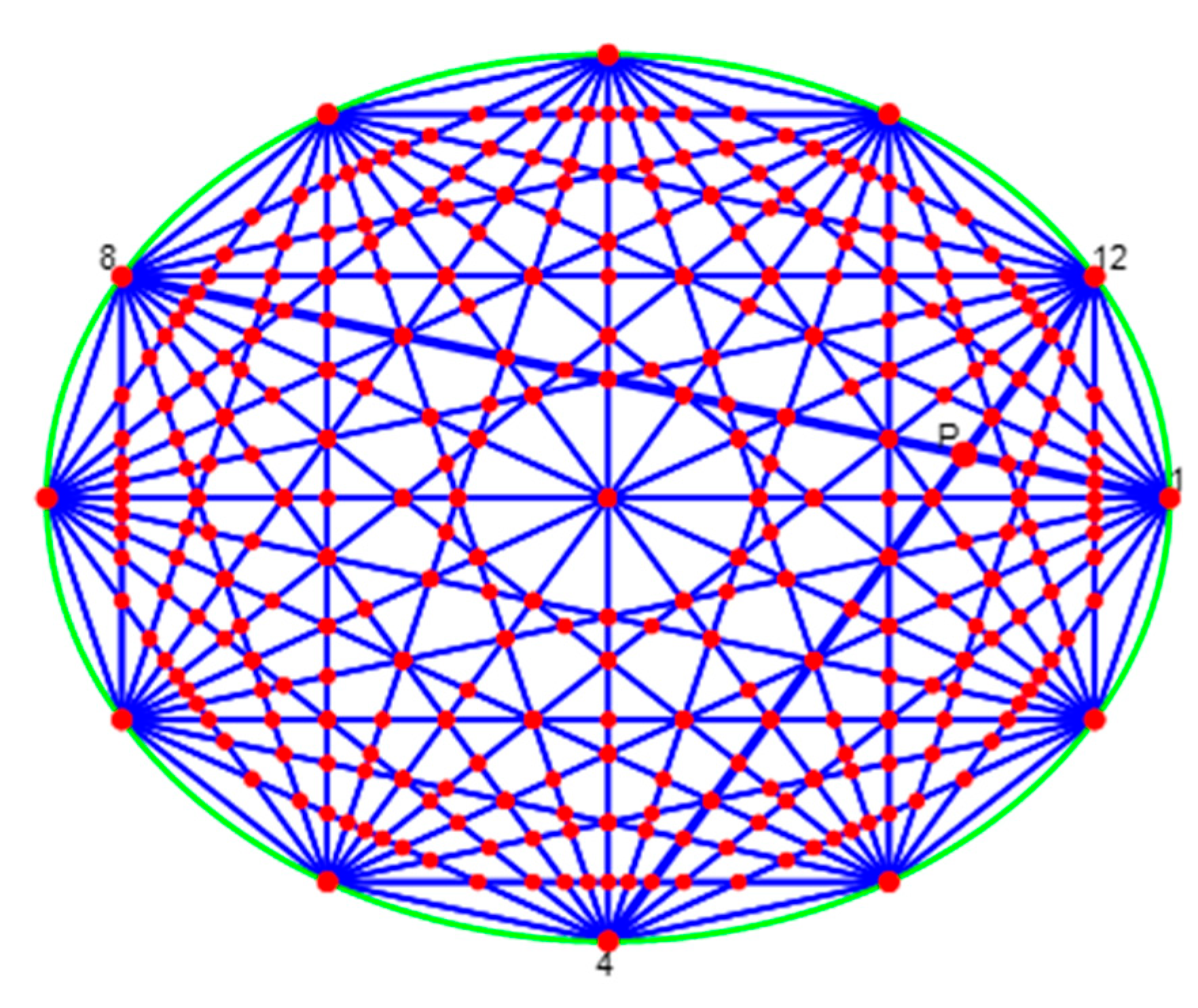
3.2.1. Azimuth Search Method

In traditional IDW algorithms, the attribute value of a predicted point is calculated using only the nearest known points, without considering the orientation of these points relative to the predicted point. This can result in deviations from the true values. To address this, this paper introduces the azimuthal search method to enhance the selection of known points. The orientation search method includes several types, such as quadrilateral, hexagonal, and octagonal quadrant searches. The more refined the orientation, the more reference points are considered. The quadrilateral quadrant search divides the plane into four quadrants based on the horizontal and vertical coordinates of the predicted point. The nearest known sample points in each quadrant are selected. If a quadrant lacks suitable known points, the algorithm uses points from the remaining three quadrants for interpolation. For example, as shown in Figure 7, if there are six known points within the search radius but none in the first quadrant, the known points from the second, third, and fourth quadrants are used for interpolation. The hexagonal and octagonal quadrant searches follow similar principles, with the octagonal method providing the highest level of refinement. Despite its complexity, the octagonal quadrant search yields the most accurate attribute values for the predicted points. Therefore, this paper employs the octagonal quadrant search method.

3.2.2. Eccentric Circle Search Method

Under normal circumstances, the azimuth search method involves drawing a circle centered on the predicted point, dividing it into several quadrants within the search radius, and selecting the nearest known point in each quadrant to calculate the attribute value of the predicted point. However, because knots are typically located near the periphery of the log cross-section, the distribution of known points may be uneven. For example, if a predicted point Q is situated at a knot location, and the known points in its search radius include one P that is not at a knot location but is the closest to Q within its quadrant, the normal azimuth search method may result in inaccuracies. In such cases, the known point P, while being closest, has minimal influence on the predicted point Q. This can cause significant deviations between the obtained and true results. To address this issue, the paper combines the traditional azimuth search method with an azimuth search method based on eccentric circles. An eccentric circle is a circle whose center is not at its geometric center. This combined approach allows for more accurate screening of known points by considering the spatial distribution of knots and selecting the most appropriate search method for different predicted point locations. This method helps to minimize deviations and improve the accuracy of the attribute values calculated for the predicted points.

To estimate the attribute values of points on the cross-section of the sample log, the cross-section is divided into two regions based on the half of the mean radius. Points located within 1/2R from the center are classified as being in the central region, while points located outside 1/2R are in the outer region. For points in the central region, the attribute values are calculated using the normal azimuthal search method to screen known points. For points in the outer region, the eccentric circle-based search method is used for screening. To determine the appropriate method for each estimated point, first, assess whether the point is within half of the average radius of the cross-section. The method for this determination is as follows:

$$f\left(x,y\right)=\left\{\begin{array}{c}1,\mathrm{sqrt}\left(x^2+y^2\right)>R/2\\ 0,\mathrm{sqrt}\left(x^2+y^2\right)\le R/2\end{array}\right.$$

(2)

where $x$ and $y$ are the coordinates of the estimated point, and R is the average radius of the cross-section of log. If the value of $f\left(x,y\right)$ is 1, it means that the estimated point is located in the outer region, and a radial search method based on eccentric circles needs to be used to screen the known points. As shown in Figure 8, point $M\left(x_1,y_1\right)$ is the estimated point, point $N\left(x_2,y_2\right)$ is the geometric center of the eccentric circle centered at point $M$, and the center of the cross-section of the log is point $O$, which is on the line $MN$. Therefore, a search radius r must be selected, with point N as the center, to define an area for filtering known points. As shown in Figure 8, four known points are located within this defined area. The eccentric circle is then divided into multiple quadrants with point M as the center. These four known points are filtered based on their distances relative to point M, and the attribute value of the estimated point is calculated. The farther point M is from the center of the sample log’s cross-section, the greater the deviation of the eccentric circle’s center, and the longer the distance from point M to point N. Since this eccentricity is related to the distance from point M to the center of the log’s cross-section, the eccentricity can be expressed as follows:

$$p=\left(d-R/2\right)/R$$

(3)

where $p$ is the degree of eccentricity, $d$ is the distance between the estimated point $M$ and the center point $O$ of the cross-section of the sample log, and $R$ is the average radius of the cross-section of the sample log.

The determination of eccentricity plays an important role in the calculation accuracy of the interpolation algorithm. The horizontal and vertical coordinates of the geometric center point $N$ of the eccentric circle can be calculated through the eccentricity $p$, and the calculation method is as follows:

$$\left\{\begin{array}{c}{x}_2=x_1+x_1\times p\\ y_2=y_1+y_1\times p\end{array}\right.$$

(4)

In the formula, $x_2$ and $y_2$ are the horizontal and vertical coordinates of $N$ points, respectively; $x_1$ and $y_1$ are the horizontal and vertical coordinates of point $M$; and $p$ is the eccentricity of the eccentric circle. After determining the coordinates of the geometric center N of the eccentric circle, select a search radius and draw a circle with point N as the center to define the area for filtering known points. The plane is divided into multiple quadrants based on the horizontal and vertical coordinates of the estimated point M. In each quadrant, the known sample points closest to the estimated point M are selected. If no known sample points meet the conditions in a particular quadrant, only the known sample points from other quadrants are used as reference points to calculate the attribute value of the estimated point M. The calculation method is as follows:

$$Z_M={\displaystyle \frac{{{\displaystyle \sum }}_{i=1}^n(w_i{Z}_i)}{{{\displaystyle \sum }}_{i=1}^n{w}_i}}$$

(5)

where $Z_M$ represents the attribute value of the estimated point; $n$ represents the number of known points searched; $Z_i$ represents the attribute value of the $i$th known point; and $w_i$ represents the weight of the $i$th known point, that is, the degree of influence of the attribute value $Z_i$ of the $i$th known point on the attribute value $Z_M$ of $M$, which is inversely proportional to the distance between the known point and the estimated point $M$:

$$w_i=k{\displaystyle \frac{1}{d_i^q}}$$

(6)

where $q$ is the power of distance and is a positive real number. $k$ is a real number greater than 0. The value of $q$ will seriously affect the result of spatial interpolation. If the value of $q$ is too small and close to 0, then the attribute value of the predicted point will be close to the average of the attribute values of all known points. If the value of $q$ is too large, the estimated point will approximate the value of the nearest known point. In this case, the nearest distance method can be regarded as a special case of the reverse-distance-weighting method. In the actual application process, the selection criterion of $q$ value is related to the minimum average absolute deviation, which usually was two. By substituting Equation (5), the attribute value of $M$ of the predicted point can be obtained as follows:

$$Z_M={\displaystyle \frac{{\sum }_{i=1}^n\left(\frac{Z_i}{d_i^q}\right)}{{\sum }_{i=1}^n\left(\frac{1}{d_i^q}\right)}}$$

(7)

If the value of f(x,y) in Equation (2) is zero, it indicates that the estimated point is located in the central area, and the standard azimuth search method is used to filter known points. As shown in Figure 9, point M represents the estimated point. With point M as the center, a circle is drawn using a selected search radius to define the area for filtering known points. The search area is divided into multiple quadrants, with point M as the center. In each quadrant, only the known points closest to the estimated point M are selected to calculate its attribute value. If no known sample point meets the conditions in a given quadrant, only the known sample points from other quadrants are used as reference points to compute the attribute value of the estimated point. The attribute value of the estimated point M is then calculated using Equation (7).

3.3. ECIDW Algorithm Imaging Steps

Step 1: Input the collected resistance data.

Step 2: Input the coordinates of 12 measurement positions, calculate the intersection coordinates of the resistance line segments in the wood cross-section, and assign the corresponding resistance value of the intersection as its attribute value.

Step 3: Select 1000 estimated points $Q\left(xi,yi\right)\left(i, 1, 2, 3, \dots , 1000\right)$ evenly distributed in the cross-section of the sample log. Use Equation (2) to determine if the point is in the central or outer region. If the result is 0, proceed to Step 4. If the result is 1, proceed to Step 5.

Step 4: For predicted point $Q\left(xi,yi\right)$ in the central region, calculate the distance between Q and all known points within the search radius. Use the eight-quadrant search method to filter the relevant known points. Apply Equation (7) to calculate the attribute value of Q.

Step 5: For predicted point $Q\left(xi,yi\right)$ in the outer region, determine the geometric center coordinate $P\left(xi,yi\right)$ of the eccentric circle centered at $Q\left(xi,yi\right)$ using Equations (3) and (4). Calculate the distance between Q and all known points within the search radius with P as the center. Screen the known points using the azimuth search method based on the eccentric circle. Use Equation (7) to calculate the attribute value of Q.

Step 6: Assign colors to the estimated points based on their attribute values. Visualize the data in two dimensions.

4. Results and Analyses

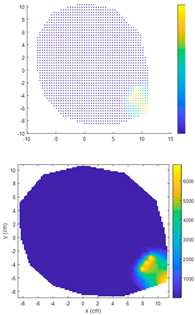
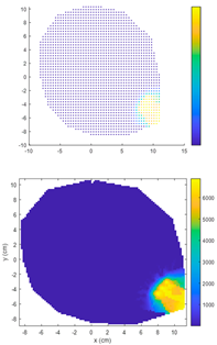
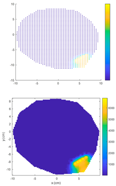
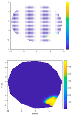
4.1. Comparison of Electrical Resistance Tomography Results Between IDW Algorithm and ECIDW Algorithm

In this paper, conventional IDW and improved ECIDW algorithms are used to compare the imaging results of sample logs with varying sizes, shapes, and numbers of knots. The algorithm imaging results are presented in

Table 2. Resistance tomography results of single-section sample log.

Specimen Log Number	IDW Algorithm	ECIDW Algorithm

and

Table 3. Resistance tomography results of two-node subsample log.

Specimen Log Number	IDW Algorithm	ECIDW Algorithm

. Each table contains two graphs showing the imaging effect for each sample log. The upper graph displays all the nodes generated by the interpolation algorithm, while the lower graph shows the two-dimensional visualization of the nodes. To present the tomographic imaging clearly, a three-color scheme is used to represent the internal conditions of the sample logs. Yellow indicates the highest resistance, green represents the median, and blue signifies the lowest resistance. The color range spans from yellow to blue, with all node resistance values evenly distributed within this spectrum. Therefore, blue represents areas of low resistance and healthy wood; green indicates areas with higher resistance and potential defects; and yellow signifies the highest resistance, corresponding to knots in the wood.

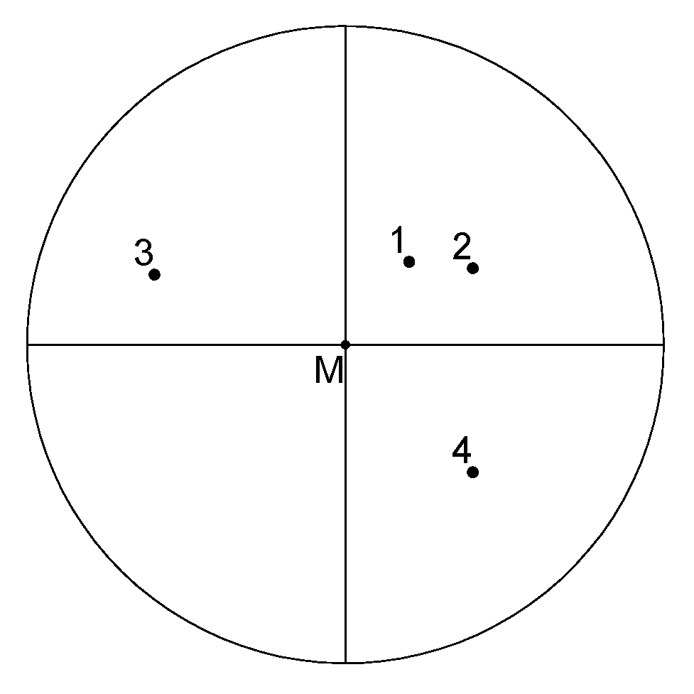
4.1.1. Single-Knot Specimen Logs

Table 2 presents the tomographic imaging results for sample logs with a single knot. The position, size, and shape of the knots vary for each sample log. The results of the two imaging algorithms for sample logs 1, 2, and 3, which have a single knot, are shown in Table 2. Notably, sample logs 1 and 2 are pine, while sample log 3 is fir. For sample logs with a single knot, both the conventional IDW and the improved ECIDW algorithms accurately predict the location of the knot. However, neither algorithm can precisely predict the shape of the knot. There remains a discrepancy between the knot shapes predicted by the algorithms and the actual knot shapes. Differences in the detection of the knot’s shape and area are also observed between the two algorithms. As seen in Table 2, the knot shape and area detected by the ECIDW algorithm align more closely with the actual knot characteristics compared to those detected by the IDW algorithm. For sample log 3, both algorithms successfully detect the approximate location of the knot area, but deviations are evident in the shape and size estimates. In the IDW algorithm’s tomographic image, the identified knot area is very subtle, which significantly differs from the actual knot area. In contrast, the ECIDW algorithm’s tomographic image shows a knot area that more closely matches the actual log than the IDW algorithm’s image, but it still does not fully align with the real knot. This discrepancy occurs because the knot area in sample log 3 is relatively small, leading to fewer known nodes within the knot area. Consequently, the number of interpolated nodes located in the knot area is also small, resulting in a significant difference between the tomographic imaging results and the actual knot characteristics.

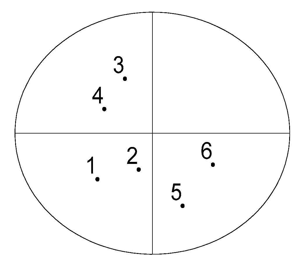
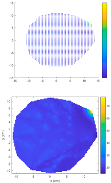
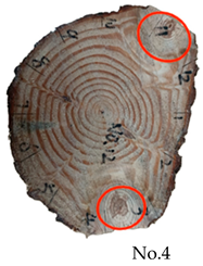
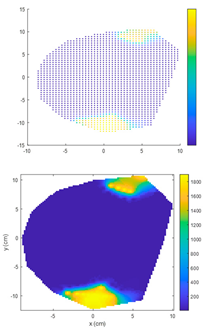
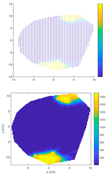
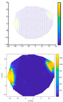
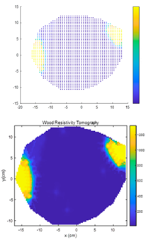
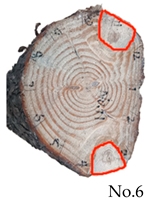
4.1.2. Double-Knot Specimen Logs

Table 3 presents the tomographic imaging results for sample logs with two knots. The location, size, and shape of the knots vary for each sample log. The results of two different imaging algorithms for sample logs 4, 5, and 6, which are all pine logs with two knots, are shown in Table 3. For these logs, both the conventional IDW algorithm and the improved ECIDW algorithm accurately predict the location of the knots, except for sample log 6. However, there are still differences between the two algorithms in predicting the shape and area of the knots. In the case of sample log 6, both algorithms can only predict the knots in the lower area of the log’s cross-section, while the knots in the upper area are not reflected in the imaging results. This discrepancy may be due to inaccurate resistance data collected from the irregular trunk. Although the resistance data collected in the knot area are higher than in the healthy area of the cross-section, they are much lower than the resistance data from the knots in the lower part of the cross-section. As a result, the knot in the upper area appears light blue in the tomographic image—different from the healthy area—but it does not show the yellow typically associated with knots. Similarly, for sample logs 4, 5, and 6, whether using the IDW algorithm or the ECIDW algorithm, the shape of the knots cannot be predicted with high accuracy. The knot shapes obtained by both imaging algorithms differ from the actual knot shapes of the logs, consistent with the results for single-knot logs. Identifying the reasons behind these discrepancies in knot shape and improving the accuracy of shape prediction will be the focus of further research.

4.2. Analysis of the Results of the Prediction of the Size of the Knot Area of the Specimen Logs

To more intuitively compare and analyze the precision and accuracy of the IDW and ECIDW algorithms in predicting the size of knots (i.e., the area of knots), the areas of knots identified in the tomographic images obtained by both algorithms were measured and calculated. This approach allowed for a comparison of the knot areas across six sample logs under both algorithms, as well as the calculation of the relative error between the predicted knot areas and the actual knot areas.

The method used to calculate the knot area in the sample logs via the tomography algorithm involves determining the ratio of the points in the yellow defective region of the tomographic image to the cross-sectional area of the measured sample logs. This ratio is then multiplied by the cross-sectional area to yield the estimated knot area in the tested sample logs. The calculation is performed using the following formula:

$$S_i={\displaystyle \frac{S\times n^{\prime }}{X}} i=1,2$$

(8)

where $S_i$ is the area of the nodal region of the tested sample log calculated by the tomography algorithm, $S$ is the area of the cross-section corresponding to the tested sample log, $n^{\prime }$ is the number of points in the nodal region in the cross-section, and $X$ is the total number of interpolated points.

In addition, based on the measured nodule areas of the specimen logs given in Table 1 and the nodule areas of the specimen logs under the tomography algorithm calculated by Equation (8), the relative error between the nodule areas obtained by the tomography algorithm and the measured nodule areas can be obtained by Equation (9).

$$D_{t_i}={\displaystyle \frac{\left|S^{\prime }-S_i\right|}{S^{\prime }}} i=1,2$$

(9)

In the above equation, $S^{\prime }$ is the knot area of the specimen log obtained by actual measurement, $S_1$ is the knot area of the specimen log obtained using the IDW algorithm, and $S_2$ is the knot area of the specimen log obtained using the ECIDW algorithm. $D_{t_1}$ is the relative error between the knot area of the specimen log obtained by using the IDW algorithm and the actual area of the measured knot, and $D_{t_2}$ is the relative error between the knot area of the specimen logs calculated by the ECIDW algorithm and the real area of the measured knot. The results of the above-related calculations are shown in

Table 4. Test results of sample node defects.

Specimen Log Number/No.	Measured Nodule Area ${\mathit{S}}^{\prime }/\mathbf{c}{\mathbf{m}}^2$	The IDW Algorithm Is Calculated to Obtain the Nodal Area ${\mathit{S}}_1/\mathbf{c}{\mathbf{m}}^2$	The ECIDW Algorithm Is Calculated to Obtain the Nodal Area ${\mathit{S}}_2/\mathbf{c}{\mathbf{m}}^2$	Relative Error of IDW Algorithm ${\mathit{D}}_{{\mathit{t}}_1}/\mathit{\%}$	Relative Error of ECIDW Algorithm ${\mathit{D}}_{{\mathit{t}}_2}/\mathit{\%}$
1	18.14	6.10	15.99	66.37	11.85
2	26.49	17.99	21.34	32.09	19.44
3	7.12	0.83	1.84	88.34	74.16
4	34.80	28.20	33.99	18.97	2.33
5	55.59	43.08	54.58	22.50	1.82
6	29.24	10.91	13.73	62.27	53.04

.

Table 4 presents the measured knot areas, calculated knot areas, and the relative errors for six specimen logs. Compared to the IDW algorithm, the ECIDW algorithm accounts for the fact that most wood knots are located near the periphery of the wood cross-section. It incorporates both the azimuth search method and the eccentric circle search method to filter known points. Using the azimuth search method, the ECIDW algorithm filtered only eight points. The known points are interpolated based on orientation, and the filtered points are more closely related to the interpolation points in terms of attributes. The ECIDW algorithm takes more factors into consideration when filtering known points than the IDW algorithm. When calculating the attribute values of interpolation points, both algorithms assign weights based on the distance from the known points to the interpolation points and perform a weighted average to determine the final attribute values. However, if the distribution of known points is relatively dense, the computational cost of the IDW algorithm, which interpolates based on all points within the search range, will be significantly higher than that of the ECIDW algorithm. According to experimental data and theoretical analysis, the ECIDW algorithm is more accurate than the IDW algorithm in most cases. This improvement in accuracy can significantly reduce errors and material waste in many industrial applications, resulting in substantial overall benefits.

The relative error Dt₁ of the knot areas obtained using the IDW algorithm ranges from 18.97% to 88.34%, with an average relative error of 48.42%. The smallest relative error is 18.97% for specimen log No.4, while the largest is 88.34% for specimen log No.3. For specimen logs 1, 3, and 6, the relative errors exceed 60%, indicating substantial discrepancies between the predicted and actual knot areas. In comparison, the relative error Dt₂ for the ECIDW algorithm ranges from 1.82% to 74.16%, with an average relative error of 28.10%. For specimen log No.1, No.2, No.4, and No.5, the relative errors are within 20%, and for specimen logs 4 and 5, the errors are less than 5%, demonstrating high accuracy. However, for specimen log No.3 and No.6, the relative errors are relatively higher at 74.16% and 53.04%, respectively. Overall, the ECIDW algorithm consistently achieves lower relative errors compared to the IDW algorithm. This indicates that the ECIDW algorithm provides more accurate imaging results, aligning more closely with the actual knot areas in the specimen logs. The IDW algorithm, by contrast, shows larger discrepancies, suggesting its imaging performance is less reliable than that of the ECIDW algorithm.

It should be especially noted here that for specimen log No.3, the relative errors $D_{t_1}$ and $D_{t_2}$ of the nodal area obtained by the IDW algorithm and ECIDW algorithm are 88.34% and 74.16%, respectively, which means that, regardless of which algorithm is used, the relative errors are larger, which may be due to the fact that the nodal area of specimen log No.3 is relatively small, so there are fewer known defective points located in the nodal area and the number of all nodes located on the nodal area obtained through the interpolation of all the nodes located in the node region is also less, resulting in the tomographic imaging results and the actual sample log differences. The use of the ECIDW algorithm for such sample log cross-section imaging will have a large error, and combined with the imaging results from Table 3, the ECIDW algorithm imaging in the node position basically conforms to the actual location of the node, but the size of the area is different from the actual area of the knots, so the accuracy of the two algorithms for imaging such samples is not high. In addition, for specimen log No.6, the relative error $D_{t_2}$ of the ECIDW algorithm is relatively large, 53.04%, which may be caused by the inaccuracy of the collected resistance data due to the irregularity of the tree trunk. The ECIDW algorithm determines the location and approximate area size of the knots below the cross-section, but the judgement of the knots above the area is biased, and the resistance data collected from the knots above the section are higher than from the healthy area of the cross-section, though the resistance data are higher from than the healthy area of the cross-section. The resistance data collected in the area of the node located above the cross-section are higher than from the healthy area of the cross-section, but much smaller than the resistance data in the area of the node below the cross-section. Combined with the imaging results in Table 3, it can be seen that the light blue color is shown on the area of the node above the tomographic image, which is different from that of the healthy area, but it does not show the yellow color as that of the area of the node below the cross-section.

In summary, from the results of resistance imaging and computational analysis of the six specimen logs, it can be seen that the average prediction accuracy of predicting the knot area of specimen logs using the IDW algorithm is only 51.58%, whereas the average detection accuracy of predicting the knot area of specimen logs using the ECIDW algorithm is 72.90%, i.e., the accuracy of predicting the knot area of the ECIDW algorithm, which is improved in this paper, is higher than that of the conventional IDW algorithm. Knots in wood not only affect its appearance but also make processing more challenging. The ECIDW algorithm can accurately identify the exact location of knots and estimate their size and shape more precisely in most cases. This algorithm enhances the accuracy of knot detection, reduces misjudgments, and minimizes wood waste caused by knots. As a result, it improves product quality while lowering costs related to rework and material waste. As the continuous advancement of automation and intelligence in wood processing, the ECIDW algorithm could be further integrated into smart factory systems, helping the industry evolve toward greater efficiency and sustainability. By integrating with Internet of Things (IoT) devices and big data platforms, the ECIDW algorithm can process large volumes of data in real time, support automated decision-making, and improve traditional wood processing methods. However, both the IDW and ECIDW algorithms may lack precision in predicting knot shapes. When dealing with irregular shapes or complex structures, they may fail to capture subtle shape variations, leading to prediction errors. Kriging interpolation, a statistical method that accounts for spatial autocorrelation, can improve prediction accuracy. In the future, it may be beneficial to combine kriging interpolation with the orientation search method and the eccentric circle search method introduced in this paper to enhance knot shape prediction and improve the overall accuracy of the algorithm.

5. Conclusions

In this paper, an improved ECIDW algorithm is proposed for application in the non-destructive detection of log knots using electrical resistance measurements. The algorithm’s performance is assessed through two-dimensional tomographic imaging of internal log knots and compared with the results obtained using the traditional IDW algorithm. The following conclusions are drawn:

(1)

For the sample logs, both the conventional IDW algorithm and the improved ECIDW algorithm can accurately predict the location of the knots, but the shape of the knots cannot be accurately predicted by both of them. At the same time, there is a difference between the knot shapes obtained by the algorithms and the actual knot shapes.

(2)

The relative error $D_{t_1}$ for the knot area measured by the IDW algorithm ranges from 18.97% to 88.34%. In comparison, the relative error $D_{t_2}$ for the knot area measured by the ECIDW algorithm varies from 1.82% to 74.16%. Overall, for the specimen logs, the relative errors of the knot areas calculated using the ECIDW algorithm are consistently smaller than those obtained using the IDW algorithm. This indicates that the knot tomography imaging accuracy of the ECIDW algorithm is superior to that of the IDW algorithm.

(3)

Using the IDW algorithm to predict the knot area of specimen logs yields an average prediction accuracy of only 51.58%. In contrast, the ECIDW algorithm proposed in this paper achieves an average detection accuracy of 72.90%. This demonstrates that the improved ECIDW algorithm provides a significantly higher accuracy in predicting the knot area compared to that of the conventional IDW algorithm.

References

- Zheng, Q.; Zhao, W.; Xu, F.; Liu, Y. Stress wave wood defect tomography based on asymmetric ellipse. J. For. Eng. 2023, 8, 137–143. [Google Scholar]
- Wang, Z.; Fang, Y.; Feng, H.; Du, X.; Xia, K. Methods for detecting and locating knot defects in wood. Prog. Laser Optoelectron. 2018, 55, 317–324. [Google Scholar]
- Huang, S.; Wang, J.; Lu, J.; Lei, Y. Research progress of world knot. For. Prod. Ind. 2011, 38, 3–7. [Google Scholar]
- Oja, J. Evaluation of knot parameters measured automatically in CT-images of Norway spruce (Picea abies (L) Karst). Holzals Roh Und Werkst. 2000, 58, 375–379. [Google Scholar] [CrossRef]
- Nordmark, U. Models of knots and log geometry of young Pinus sylvestris sawlogs extracted from computed tomographic images. Scand. J. For. Res. 2003, 18, 168–175. [Google Scholar] [CrossRef]
- Thomas, R.E. Predicting intemal Yellow-poplar log defect features using surface indicators. Wood Fiber Sci. 2008, 40, 14–22. [Google Scholar]
- Dong, F.; Cui, X. Development of resistance tomography. Chin. J. Sci. Instrum. 2003, 35, 703–705. [Google Scholar]
- Bao, Z.; Wang, L. Research progress on the application of resistance test method in wood decay detection. For. Eng. 2013, 29, 47–51. [Google Scholar]
- Just, A.; Jacbbs, F. Elektrische Widerstandstomographie zur Umersuchung des Gesundheitszustandes von Baumen. Hochaufl6sende Geoelektrik Leipz. Inst. Flit Geophys. Geol. 1998, 1, 2–3. [Google Scholar]
- Weihs, U.; Dubbel, V.; Knunmheuer, F.; Just, A. The electrical resistivity tomography—A promising technique for the detection of colored heart wood on standing beech trees. Forst Holz 1999, 54, 166–170. [Google Scholar]
- Lin, C.J.; Chung, C.H.; Yang, T.H.; Lin, F.C. Detection of electric resistivity tomography and evaluation of the sapwood-heartwood demarcation in three Asia Gymnosperm species. Vestn. Khirurgii Im. I.I.Grek. 2012, 46, 33–37. [Google Scholar] [CrossRef]
- Bicker, D.; Rust, S. Electric resistivity tomography shows radial variation of electrolytes in Quercus robur. Can. J. For. Res. 2010, 40, 1189–1193. [Google Scholar] [CrossRef]
- Adrien, G.; Ostergaard, K.T.; Mothei, L.; Fan, J.; Lockington, D.A. Using electrical resistivity tomography to differentiate sapwood from heartwood: Application to conifers. Tree Physiol. 2013, 45, 187–194. [Google Scholar]
- Yue, X.; Wang, L.; Wang, X.; Rong, B.; Ge, X.; Liu, Z.; Chen, Q. Quantitative detection of decay degree of living wood by three nondestructive testing methods: Resistance tomography and Stress sweep and impedance meter. Chin. J. For. 2017, 53, 138–146. [Google Scholar]
- Shi, X.; Wang, L.; Xu, H.; Xu, Q.; Cao, S.; Xu, M. Quantitative detection of internal decay of red pine based on impedance meter and ERT technology. J. Beijing For. Univ. 2017, 39, 102–111. [Google Scholar]
- Liu, G.; Wu, Y.; Yang, J.; Yu, S. Three-dimensional spatial variation of regional soil salinity based on spectral index. Spectrosc. Spectr. Anal. 2013, 33, 2758–2761. [Google Scholar]
- Wang, Y.; Ding, Y.J.; Ye, B.S.; Liu, F.; Wang, J.; Wang, J. Contributions of climate and human activities to changes in runoff of the Yellow and Yangtze rivers from 1950 to 2008. Sci. China Earth Sci. 2013, 56, 1398–1412. [Google Scholar] [CrossRef]
- Chen, D.; Zou, C.; Wang, S.; Li, H.; Zhang, X. Study on spatial interpolation of the average temperature in the Yili River Valley based on DEM. Spectrosc. Spectr. Anal. 2011, 31, 1925–1929. [Google Scholar]
- Chen, F.; Feng, H.; Du, X.; Fang, Y.; Weng, X. Three-dimensional stress wave imaging method of wood internal defects based on TIDW. Chin. J. Sens. Technol. 2015, 28, 1625–1633. [Google Scholar]
- Duan, Z.-G.; Xiao, H.-S.; Yuan, W.-X. Interpolation method of forest canopy height model based on discrete point cloud data. Sci. Silvae Sin. 2016, 52, 86–94. [Google Scholar]
- Fan, Y.; Yu, X.; Zhang, H.; Song, M. Comparative analysis of Kriging and IDW interpolation of rainfall data: A case study of Lijiang River Basin. J. Hydrol. 2014, 34, 61–66. [Google Scholar]