Sawing Model and Optimization of Single Pass Crosscut Parameters for Pinus kesiya Based on the Transformer Model

Abstract

The optimization of the sawing process for Pinus kesiya Royle ex Gordon, an important timber used in construction and furniture, especially through the adjustment of parameters such as wood moisture content, cutting speed, and feed speed, not only helps reduce energy consumption and noise but also improves surface processing quality, thereby promoting green and environmentally friendly production. Therefore, this study selects the wood moisture content, cutting speed, and feed speed during the Single Pass Crosscut process of Pinus kesiya as the preliminary experimental parameters. Based on the Transformer model, a cutting prediction model for Pinus kesiya is established to predict three cutting performance indicators: cutting power consumption, surface roughness, and cutting noise. Meanwhile, Bayesian optimization was used to search for the optimal parameter combination within the specified cutting process parameter ranges that minimizes the objective function for these cutting performance indicators. Finally, experimental verification based on the optimal parameter combination shows that the average coefficient of determination for the cutting performance indicators is 0.937, the average mean squared error is 0.076, and the average mean absolute error is 0.186, indicating good agreement between the predicted and measured values.

1. Introduction

Pinus kesiya, as a high-quality pine species, is widely used in construction, furniture, and decorative materials due to its straight trunk, excellent wood quality, rapid growth, and attractive grain patterns [1]. However, during processing, the sawing stage is a core step with high energy consumption, and the Single Pass Crosscut is an indispensable part of this process. Therefore, optimizing the Crosscut process parameters for Pinus kesiya is not only an important approach to achieving low-energy, low-noise green production but also a key measure to expand its application fields and improve product quality [2]. Studies have shown that as the moisture content of wood increases, cutting resistance, noise levels, and surface roughness all rise significantly [3,4,5,6]. Although faster feed speeds can improve processing efficiency, they also lead to a significant increase in power consumption when sawing pine wood [7,8]. During high feed speeds, the reduced contact time between the tool and the workpiece results in increased surface roughness, lower surface quality, and higher sawing power consumption [9,10,11]. An appropriate cutting speed can, to some extent, reduce sawing noise while improving the quality of the sawn surface [12,13]. Therefore, exploring the optimal pre-experimental parameters for sawing Pinus kesiya, such as moisture content, feed rate, and cutting speed, is the core issue in optimizing the Crosscut process using circular saws. This approach aims to effectively reduce sawing power consumption and noise while improving the surface roughness of the cut.

In recent years, backpropagation neural network (BP) development has solved the problem of optimizing sawing parameters [14]. For example, Cus and Zuperl used a standard feed-forward neural network with BP learning rules and a radial-based neural network to achieve multi-objective optimization of cutting parameters by considering the prediction results of multiple objectives, such as productivity, machining cost, and surface quality, which improved the efficiency and stability of the machining process [15]. Subsequently, scholars integrated particle swarm algorithms based on BP to predict energy consumption, surface roughness, and noise value. The particle-swarm-optimized back propagation neural network (PSO-BP) exhibits higher prediction accuracy, greater stability, and better fitting than BP [16,17,18]. However, PSO-BP depends more on feature engineering and usually requires complex preprocessing and feature extraction of input data to improve model performance, greatly increasing the development time and complexity [19,20]. Meanwhile, as an emerging self-supervised deep learning technique, the Transformer model shows great potential in multivariate and nonlinear data prediction due to its unique architecture and powerful learning capability [21]. The model’s self-attention mechanism can automatically learn and capture complex relationships between different features and efficiently handle data noise without additional feature engineering [22,23]. Numerous scholars have developed high-precision and adaptable Transformer models with strong generalization ability and robustness for their respective industries based on the Transformer’s deep learning approach, such as the DeepTTA model for predicting cancer drug response [24], models for improving the prediction of heart disease [25], models for evaluating the performance of traffic, exchange rates, electricity, and solar energy [26], etc. However, the application of Transformer models in the Single Pass Crosscut modeling of Pinus kesiya, as well as in the optimization of preliminary experimental parameters for three sawing performance metrics—cutting power consumption, surface roughness, and sawing noise—remains relatively limited. Its predictive accuracy and precision are yet to be verified.

In summary, this study focuses on the Single Pass Crosscut issue of Pinus kesiya and develops a sawing prediction model based on a Transformer framework. By integrating a Bayesian optimization algorithm, the optimal parameter combination is identified within the parameter space, ultimately forming a sawing optimization model. Furthermore, comparative validation against the Transformer and BSO-BP models is conducted to evaluate the accuracy and precision of the Transformer-based sawing prediction model. Practical validation and convergence analysis demonstrate the feasibility of this model in predicting optimal parameter combinations.

2. Materials and Methods

2.1. Materials

The experimental samples were selected from Pinus kesiya timber with a diameter at breast height of 30 cm, collected from the Pu’er region in Yunnan, China. Each sample measured 1200 mm (length) × 200 mm (width) × 50 mm (height). To investigate the effects of different moisture contents on the wood properties, the samples were divided into three groups, labeled as I, II, and III.

The three groups of samples were first placed in a drying oven with air circulation, set to a temperature of 103 ± 2 °C. During the drying process, the samples were weighed every 8 h to record any mass changes. When the mass difference between two consecutive weighings was less than or equal to 0.2% [27], the samples were considered to have reached a kiln-dried state, with a moisture content of 0%. At this point, the samples were quickly wrapped in cling film and stored, ensuring that their moisture content remained at 0%.

After reaching the kiln-dried state, the II group samples were subjected to a humidification process. The initial mass (m₀) of the kiln-dried samples was recorded, and the target mass (m_x) for a moisture content of 15% was calculated. The samples were then placed in a drying and humidifying chamber, with the relative humidity set to 15%. The samples were weighed every 4 h until their weight approached the target mass. When the sample mass reached the target value, the humidification process was stopped, and the moisture content of this group was brought close to 15% [28].

For the III group samples, a water immersion method was used to accelerate the attainment of a moisture content of 60%. The kiln-dried samples were completely submerged in water to ensure that moisture rapidly penetrated the wood. After immersion, the samples were removed and placed in the drying and humidifying chamber to undergo a moisture balance process until the moisture content stabilized around 60%. The moisture content was calculated using the following formula:

$$\mathrm{W}={\displaystyle \frac{{\mathrm{m}}_{\mathrm{w}}}{{\mathrm{m}}_0}}\times 100\%$$

(1)

where m_w—mass in target moisture content state (g), m₀—mass of wood in kiln-dried state (g), and W—target moisture content (%).

To ensure uniform moisture distribution within each group of samples, the moisture content was measured at various depths and regions of the uncut portions of the samples using a BSIDE moisture meter. Measurement points included the surface, center, and deepest regions of the left, middle, and right sections. The data from all measurement points were analyzed and the average moisture content of all areas was calculated to ensure the accuracy and reliability of the experimental results.

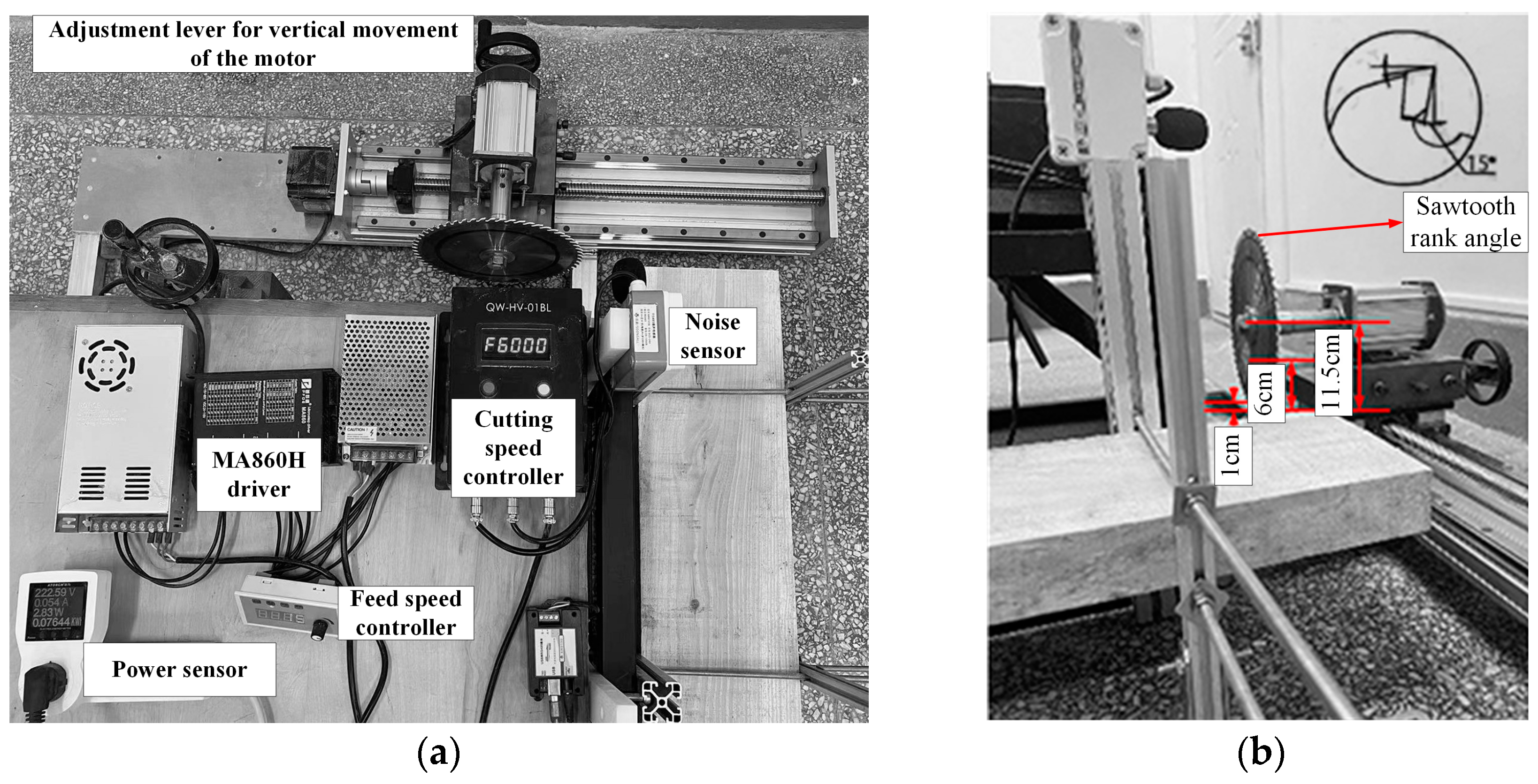
2.2. Experimental Equipment

Relevant experiments were conducted on the homemade cutting machine shown in Figure 1. The spindle motor of the cutting machine is a QW80BL007301200 brushless DC motor provided by BRUSHLESS DC MOTOR, based in Changsha, China. It has a rated power of 750 W, a maximum speed of 8000 r/min, a torque of 0.89 N·m, and an operating voltage of AC220V. This motor is equipped with an original factory inverter that enables stepless speed regulation. The control system adjusts the speed and position sensing through analog input signals and Hall effect feedback, using a simple speed control method. This control method meets our experimental requirements, providing a sufficient range of speed adjustment and satisfying the operational needs of the equipment. The feeding motor is a PERFECT brand MA860H stepper motor, based in Wenzhou, China, with an operating voltage of DC48V and a holding torque of 4.5 N·m. It is paired with the same brand’s MA860H driver and a CS10-3M pulse generator, with the pulse generator manufactured in Foshan, China, powered by WEIZHEN brand DC power supplies of 48 V and 24 V, based in Shenzhen, China. The working power monitoring sensor is directly connected to the power supply of the spindle motor and uses the WIFI function to upload real-time power consumption and time data to the mobile application software and obtains the power information of the sawed specimen through the time information before and after sawing. The noise sensor is installed above the wood that is to be sawed, at a distance of 10 cm from the surface, and connected to a computer via an RS485-to-USB converter. The sensor operates at a sampling rate of 10 Hz, outputting a decibel value processed through an A-weighted filter every second. Real-time monitoring of the sensor data can be performed using the upper computer software RV1000 (version V1.21.5.20), ensuring measurement accuracy and convenience. To minimize the effect of tool wear, three identical woodworking circular saw blade tips with OKE405 alloy heads were used in rotation, with a tooth rake angle of 15°, a tooth thickness of 2.2 mm, a blade tip arc radius of 0.8 mm, 60 teeth, and a tooth blade outer diameter of 230 mm.

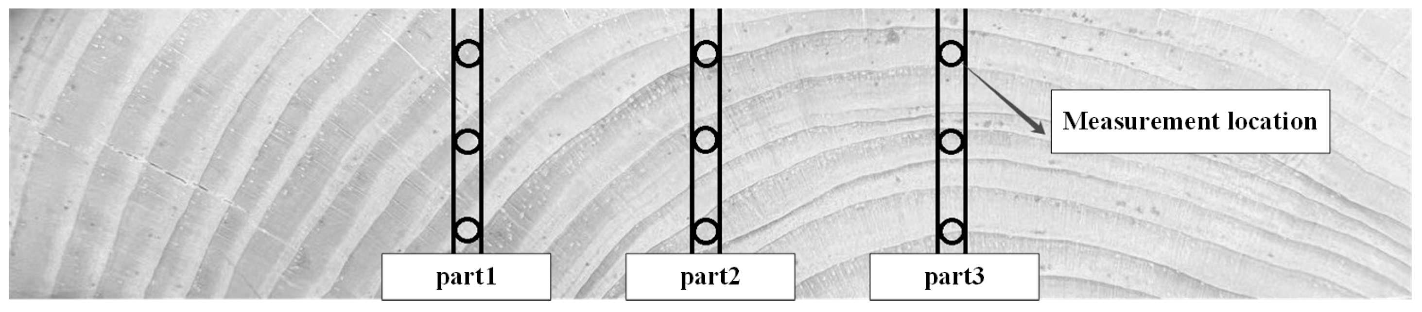
2.3. Data Collection

The tests were set up with 6 cutting speeds of 42.1497, 48.1711, 54.1925, 60.2139, 66.2352, and 72.2566 m/s, 3 feed speeds of 0.01128, 0.01686, and 0.02250 m/min, and 3 moisture contents of 0%, 15%, and 60%, and 3 levels for randomized combinations; a total of 54 test combinations were generated. For each test combination, the equivalent continuous sound level and power consumption data shown in Equations (2) and (3) were collected during the sawing process.

$${\mathrm{L}}_{\mathrm{eq}}=10\times {\log }_{10}({\displaystyle \frac{1}{\mathrm{T}}}{{\displaystyle \sum }}_{\mathrm{i}=1}^{\mathrm{n}}{10}^{{\displaystyle \frac{{\mathrm{L}}_{\mathrm{i}}}{10}}})$$

(2)

$$\mathrm{P}={\displaystyle \frac{{\mathrm{E}}_{\mathrm{a}} - {\mathrm{E}}_{\mathrm{b}}}{\mathrm{T}}}$$

(3)

where L_eq—equivalent continuous sound level (dB), T—total sawing time (s), n—number of sampling points, L_i—noise level at second i (dB), P—power consumption (kW) which, in this article, is directly equal to the sawing power, E_a—power reading before the start of sawing (kWh), E_b—power reading after the end of sawing (kWh).

The difference in water content will lead to the different densities of the samples to be tested, which in turn affects the magnitude of the roughness value of the sawn surface [29]. In the test, the equilibrium moisture content at room temperature was used as the baseline condition for the roughness test. That is, the equilibrium moisture content was considered to be reached when the weights were weighed at 10-minute intervals, and the rate of mass change between the two times was less than 0.002%/min [30]. The surface roughness R_a was determined using a TR200 stylus surface roughness tester from JITAI. The evaluation length of 12.5 mm, the cut-off value of λ_c = 2.5 mm, the display range of 0.01–100 μm, the resolution of 350 μm, and the stylus tip radius of 5 μm were selected according to the suggested method of parameter setting for surface roughness tester by Aydin Demir et al. [31]. At the same time, the surface roughness test was carried out according to the DIN 4768 (1990) standard for surface roughness measurements [32]. The frame sawing process can be unstable at the inlet and outlet of the material [33], so three fixed positions were chosen where the surface roughness measurement positions were all within 50 mm from the two end sides of the specimen, as shown in Figure 2. Three measurements were taken at each position along the direction of the feed motion, totaling nine times, and the arithmetic mean of the nine measurements was taken as the evaluation criterion for the sawing surface quality.

2.4. Model Construction

2.4.1. Sawing Prediction Model

The overall structure of the saw cut prediction model is shown in Figure 3, which consists of key components such as the embedding layer, positional encoding, Transformer Encoder, and prediction layer. In order to capture the associative semantic information present in the context, the Transformer Encoder is used to learn the table of the substructure. Take a particular piece of data in a batch as an example. The embedding layer takes the weight matrix and deviation vector and projects the input feature vector X, which consists of the three data features of the water content, cutting speed, and feed speed of Pinus kesiya in

Table A1. Experimental results under various sawing parameters.

Experiment Number	Cutting Speed Vc m/s	Feed Speed Vf m/min	Moisture Content WC %	Power Consumption PC kW	Sawing Noise N dB	Surface Quality of Sawn Surfaces Ra μm
1	42.1497	0.01128	0	0.281439	82.02593	2.249926
2	48.1711	0.01128	0	0.247065	84.09147	2.131679
3	54.1925	0.01128	0	0.230048	85.97955	1.957691
4	60.2139	0.01128	0	0.216435	89.00612	1.825889
5	66.2352	0.01128	0	0.185284	91.46176	1.767056
6	72.2566	0.01128	0	0.088432	91.64638	1.657
7	42.1497	0.01686	0	0.343652	81.77817	2.4895
8	48.1711	0.01686	0	0.325642	84.6993	2.375333
9	54.1925	0.01686	0	0.290541	86.23342	2.243389
10	60.2139	0.01686	0	0.289906	87.62488	2.146667
11	66.2352	0.01686	0	0.263774	88.57406	2.068056
12	72.2566	0.01686	0	0.250518	89.02653	1.972056
13	42.1497	0.02250	0	0.308382	83.0181	2.566222
14	48.1711	0.02250	0	0.288459	84.47476	2.434222
15	54.1925	0.02250	0	0.268968	84.88714	2.370722
16	60.2139	0.02250	0	0.249019	85.08683	2.235667
17	66.2352	0.02250	0	0.246611	90.0246	2.167611
18	72.2566	0.02250	0	0.189401	90.28651	2.058889
19	42.1497	0.01128	0.15	0.314071	92.56651	2.441417
20	48.1711	0.01128	0.15	0.297813	94.39432	2.367639
21	54.1925	0.01128	0.15	0.275719	95.06099	2.260194
22	60.2139	0.01128	0.15	0.25589	96.39702	2.156056
23	66.2352	0.01128	0.15	0.253916	97.46135	2.045139
24	72.2566	0.01128	0.15	0.23461	98.51679	1.941972
25	42.1497	0.01686	0.15	0.317478	92.95751	2.548333
26	48.1711	0.01686	0.15	0.306212	94.18668	2.459278
27	54.1925	0.01686	0.15	0.28944	95.54272	2.358389
28	60.2139	0.01686	0.15	0.277496	96.92306	2.166417
29	66.2352	0.01686	0.15	0.270889	97.95669	2.038
30	72.2566	0.01686	0.15	0.2592	99.8439	1.944944
31	42.1497	0.02250	0.15	0.352548	93.53476	2.643083
32	48.1711	0.02250	0.15	0.338704	94.4054	2.542028
33	54.1925	0.02250	0.15	0.321248	96.00056	2.476222
34	60.2139	0.02250	0.15	0.313338	97.64016	2.349444
35	66.2352	0.02250	0.15	0.302675	98.82611	2.233056
36	72.2566	0.02250	0.15	0.277223	100.3251	2.1415
37	42.1497	0.01128	0.60	0.2496	2.623444	2.605444
38	48.1711	0.01128	0.60	0.296085	94.52122	2.505222
39	54.1925	0.01128	0.60	0.393518	2.442028	2.435333
40	60.2139	0.01128	0.60	0.429677	97.05276	2.352583
41	66.2352	0.01128	0.60	0.437381	97.282	2.319944
42	72.2566	0.01128	0.60	0.45659	98.11916	2.228861
43	42.1497	0.01686	0.60	0.329061	93.3669	2.77725
44	48.1711	0.01686	0.60	0.383951	93.46133	2.630583
45	54.1925	0.01686	0.60	0.410795	95.4466	2.555889
46	60.2139	0.01686	0.60	0.436122	96.18175	2.520639
47	66.2352	0.01686	0.60	0.441544	97.01009	2.433583
48	72.2566	0.01686	0.60	0.467979	98.33269	2.325583
49	42.1497	0.02250	0.60	0.354726	94.8481	2.932611
50	48.1711	0.02250	0.60	0.446331	96.22889	2.762056
51	54.1925	0.02250	0.60	0.478691	96.23643	2.637278
52	60.2139	0.02250	0.60	0.492707	97.09175	2.530167
53	66.2352	0.02250	0.60	0.488713	98.28746	2.411056
54	72.2566	0.02250	0.60	0.465535	100.0133	2.351389

of Appendix A, to a higher 61-dimensional space by the equation ‘E = W∙X + b.’: where X is the input feature matrix with the shape (batch size = 8, feature length = 3), W is the weight matrix of the linear layer with the shape (feature length = 3, embedding dim = 512), and b is the bias vector of the linear layer with the shape (embedding dim = 512).

Position encoding adds position information to the input features by applying sine and cosine transformations to the positions, converting the input position information into a specific vector PE, and adding it to the original input feature E to obtain the input feature E′ that contains the position information, which enables the model to obtain the order information of the data points. The Transformer Encoder consists of a multi-head self-attention mechanism, a feed-forward neural network, residual connectivity, and layer normalization. In each layer, the multi-head attention mechanism first linearly transforms the input feature E′ pairs to generate the three matrices Query(Q), Key(K), and Value(V) shown in Equation (4).

$$\left.\begin{array}{c}\mathrm{Q}={\mathrm{W}}_{\mathrm{Q}}·{\mathrm{E}}^{\prime }\\ \mathrm{K}={\mathrm{W}}_{\mathrm{K}}·{\mathrm{E}}^{\prime }\\ \mathrm{V}={ \mathrm{W}}_{\mathrm{V}}·\mathrm{E}\end{array}\right\}$$

(4)

These matrices are then divided into four heads, each containing 128 dimensions. Next, the similarity between Query and Key is computed by dot product and divided by the square root of the dimensions of each header (‘${\mathrm{d}}_{\mathrm{k}}=\sqrt{128}$’) to stabilize the gradient, resulting in the Attention Score Matrix S shown in Equation (5).

$$\mathrm{S}={\displaystyle \frac{\mathrm{Q}·{\mathrm{K}}^{\mathrm{T}}}{\sqrt{{\mathrm{d}}_{\mathrm{k}}}}}$$

(5)

The maximum value is picked from the Attention Score Matrix to form the Attention Weight Matrix (AWM). Weighted summation of values using the Attention Weight Matrix yields an output O for each header, i.e., ‘O = AWM∙V’. Finally, the outputs of all the heads are spliced in the last dimension to generate a matrix of shape (batch size = 8, sequence length = 1, embedding dim = 244).

The feedforward neural network performs further nonlinear transformations of these new representations using the ReLU activation function, resulting in complex feature transformations and combinations at each position. Also, the risk of overfitting was prevented by randomly setting a portion of the input units to zero using dropout. Residual linking and layer normalization are applied after each sub-layer, where residual linking alleviates the gradient vanishing problem, thus making the deep network easier to train. In contrast, layer normalization accelerates the training speed and stability, and both work in tandem to ensure the stability and efficiency of the training.

Eventually, the prediction layer mapped the coded features to a linear layer in the output space, predicting the final sawing noise, sawing power consumption, and sawing surface roughness R_a.

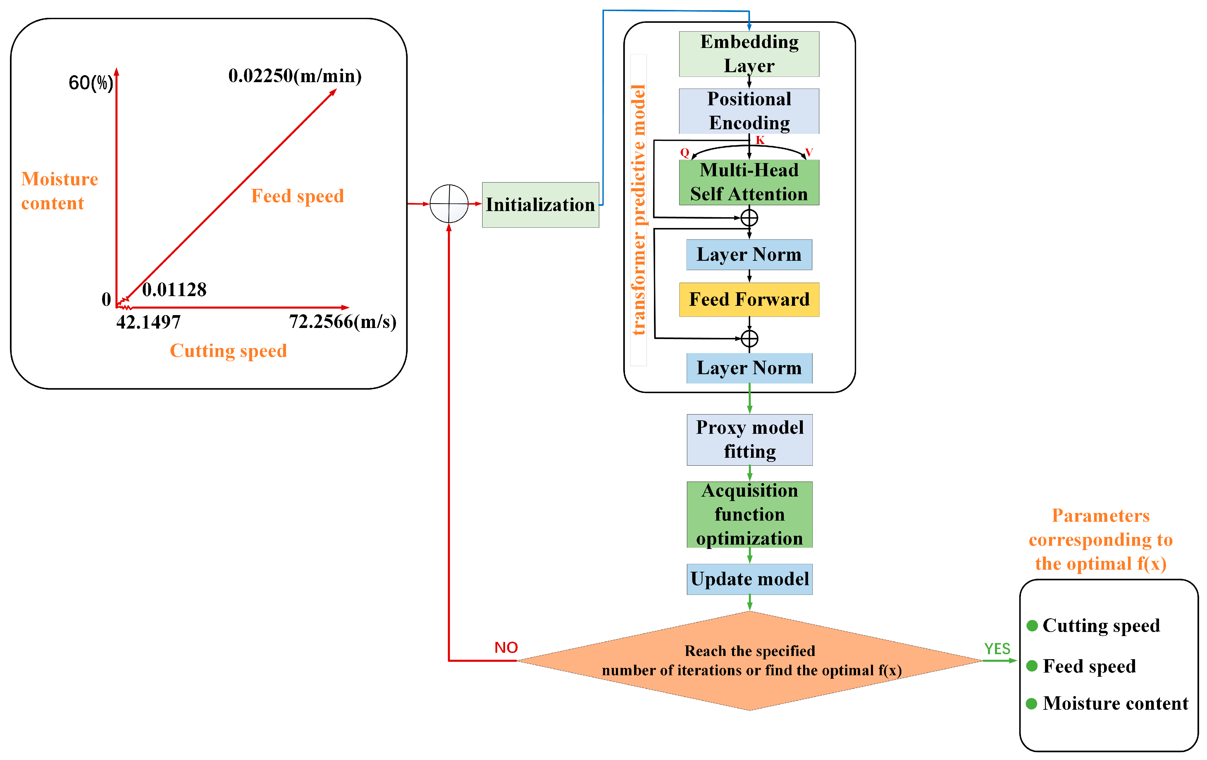
2.4.2. Sawing Optimization Model

The sawing optimization model, as shown in Figure 4, is implemented by training a surrogate model in Bayesian optimization. This model gradually optimizes the objective function f(x) (as defined in Equation (6)) based on the existing sawing prediction model, adjusting the pre-experiment parameters to ultimately determine the optimal parameter configuration. Firstly, some initial sampling points are randomly selected for the data in the input parameter space consisting of cutting speeds from 42.1497 m/s to 72.2566 m/s, feed speeds from 0.01128 m/min to 0.02250 m/min, and water content from 0% to 60%. New combinations in these spaces are inputted into the trained sawing. The corresponding power consumption, sawing noise, and sawing surface roughness R_a can be obtained from the prediction model, and the objective function f(x) of the new combination of predicted parameters is evaluated according to Equation (6). Together, these initial points and the objective function values constitute the training dataset, which is used to train the initial Gaussian process model.

$$\mathrm{f}\left(\mathrm{x}\right)=\mathsf{\alpha }·{\mathrm{P}}^2+\mathsf{\beta }·{\mathrm{Q}}^2+\mathsf{\gamma }·{\mathrm{N}}^2$$

(6)

where f(x)—evaluation function; x—parameter vector [x₁₁,x₁₂,x₁₃] consisting of consumed power (w) predicted by P, sawing surface roughness predicted by Q, and sawing equivalent noise (dB) predicted by N; α, β, γ—weighting coefficients corresponding to P, Q, and N.

In this experiment, we set α = 1000, β = 1, and γ = 1000. In other words, this sawing optimization experiment focuses on the significant optimization of power consumption and sawing equivalent noise, while achieving a slight optimization of sawing quality.

The central task of a Gaussian process model is to predict the distribution of the objective function at unsampled points by fitting it to known data. After evaluating the objective function f(x) at the initial sampling points, we use these data to train the Gaussian process. Suppose that for each given set of input points ‘X = [x₁, x₂, …, x_n]’ the corresponding to the output values ‘f(X) = [f(x₁), f(x₂), …, f(x_n)]’ all obey a multivariate Gaussian distribution with $\mathrm{N}(\mathsf{\mu }\left(\mathrm{x}\right),\mathrm{K}(\mathrm{x},{\mathrm{x}}^{\prime }\left)\right)$, where μ(x) is the mean function which is usually assumed to be 0, and $\mathrm{K}(\mathrm{x},{\mathrm{x}}^{\mathrm{\prime }})$ is the covariance function, also known as the kernel function, describing the correlation between two input points. The distribution of f(x_n+1) is obtained under the condition that X, f(X), and the new input point x_n+1 data are known, and according to the nature of the Gaussian process; the conditional distribution is still normal, with the mean $\mathsf{\mu }\left({\mathrm{x}}_{n+1}\right)$ and the variance ${\mathsf{\sigma }}^2\left({\mathrm{x}}_{n+1}\right)$ shown in Equations (7) and (8).

$$\mathsf{\mu }\left({\mathrm{x}}_{\mathrm{n}+1}\right)=\mathrm{k}{\left(\mathrm{X},{\mathrm{x}}_{\mathrm{n}+1}\right)}^{\mathrm{T}}\mathrm{K}{\left(\mathrm{X},\mathrm{X}\right)}^{-1}\mathrm{f}\left(\mathrm{X}\right)$$

(7)

$${\mathsf{\sigma }}^2\left({\mathrm{x}}_{\mathrm{n}+1}\right)=\mathrm{k}\left({\mathrm{x}}_{\mathrm{n}+1},{\mathrm{x}}_{\mathrm{n}+1}\right)-\mathrm{k}{\left(\mathrm{X},{\mathrm{x}}_{\mathrm{n}+1}\right)}^{\mathrm{T}}\mathrm{K}{\left(\mathrm{X},\mathrm{X}\right)}^{-1}\mathrm{k}\left(\mathrm{X},{\mathrm{x}}_{\mathrm{n}+1}\right)$$

(8)

Next, the gp_hedge function dynamically selects a different acquisition function to add sample points. In each iteration, one of the maximized acquisition functions is selected for the current iteration’s sample point selection based on the performance of the previous iteration and according to the probability weights from the lower confidence bound, the expected improvement, and the probability of improvement. The objective function value f(x) is computed again for the new sampling points, and the x_n+1 that performs best for one of the maximizing acquisition functions in the above selection is computed to be added to the existing training dataset (Equation (9)). The Gaussian process model is then retrained based on the updated dataset, adjusting the approximation to the objective function.

$$\begin{array}{c}{\mathrm{x}}_{\mathrm{n}+1}=\mathrm{argmin}(\mathsf{\mu }\left(\mathrm{x}\right)-\mathsf{\kappa }·\mathsf{\sigma }\left(\mathrm{x}\right))\\ {\mathrm{x}}_{\mathrm{n}+1}=\mathrm{argmin}(-\mathrm{E}\left(\max \left(0,\mathrm{f}\left(\mathrm{x}\right)-\mathrm{f}\left({\mathrm{x}}_{\mathrm{best}}\right)\right)\right))\\ {\mathrm{x}}_{\mathrm{n}+1}=\mathrm{argmin} [-{\displaystyle (}\left(\mathsf{\mu }\left(\mathrm{x}\right)-\mathrm{f}\left({\mathrm{x}}_{\mathrm{best}}\right)-\mathsf{\xi }\right)·\mathsf{\Phi }\left(\mathrm{Z}\right)+\mathsf{\sigma }\left(\mathrm{x}\right)·\mathsf{\varphi }\left(\mathrm{Z}\right){\displaystyle )}]\end{array}\hspace{1em} \}$$

(9)

where E—expectation, f(x_best)—currently known optimal value, i.e., the best point, μ(x)—predicted mean value of the model for x, σ(x)—predicted standard deviation of the model for x, Φ(Z)—cumulative distribution function of the standard normal distribution, ϕ(Z)—probability density function of the standard normal distribution, ξ and κ—adjustment parameters, which are also often referred to as exploration parameters. Higher exploration parameters lead to an increase in the weight of the exploration term and more attention to those regions with higher uncertainty when selecting sampling points, and lower exploration parameters make the optimization algorithm more inclined to use the current model’s prediction of the objective function to select those regions with better predictions or nearer to the known optimal solution for sampling.

The above process is continuously iterated and, based on the predicted mean and variance of the Gaussian process surrogate model, a new evaluation point x_n+1 is selected by the acquisition function and then the objective function is evaluated and the surrogate model is updated. This cycle continues until the set maximum number of iterations is reached or the convergence condition is satisfied. Eventually, the surrogate model is able to approximate the objective function more accurately and find the optimal solution in the parameter space.

2.5. Model Training and Validation

In the above experiment, a total of 54 data sets were obtained, 43 of them (about 79.63% of the total data) were selected as the training dataset, and the remaining 11 data (about 20.37% of the total data) were used as the test set. The saw cut prediction model uses the Mean Square Error (MSE) of Equation (2) as the loss function minimizes the MSE, updating the model parameters through the Adam optimizer. When the loss value does not decrease in one cycle, 1 counter is added and the training is stopped when the number of counters is equal to 100.

The saw cut prediction model was evaluated using three metrics of mean square error (MSE), mean absolute error (MAE) performance, and R² as shown in Equations (10)–(12). MSE is a measure of the difference between the predicted and actual values of the model and is calculated as the average of the squares of the differences between the predicted values and the actual values. MSE gives a higher weight to larger errors because the squares of errors amplify larger differences, which makes MSE more sensitive to outliers. The square of the error amplifies the larger differences, which makes the MSE more sensitive to outliers. The MAE is an important criterion for evaluating model performance that gives the same weight to all errors and can handle arbitrary true values, including zero values. As the dataset is standardized, there are more cases of data containing zero or near zero values, using MAE as one of the evaluation metrics. Regression analysis is an effective method to assess the accuracy and validity of a model through the relationship between predicted and actual values. In regression analysis, R² is a key parameter for assessing accuracy, and when R² is closer to 1, it indicates that the fit between the predictive model and the actual data is higher, and the predictive accuracy of the model is better.

$$\mathrm{MSE}={\displaystyle \frac{1}{\mathrm{n}}}{\sum }_{\mathrm{i}=1}^{\mathrm{n}}{\left({\mathrm{y}}_{\mathrm{i}} - {\widehat{\mathrm{y}}}_{\mathrm{i}}\right)}^2$$

(10)

$$\mathrm{MAE}={\displaystyle \frac{1}{\mathrm{n}}}{\sum }_{\mathrm{i}=1}^{\mathrm{n}}\left|{\mathrm{y}}_{\mathrm{i}} - {\widehat{\mathrm{y}}}_{\mathrm{i}}\right|$$

(11)

$${\mathrm{R}}^2=1 - {\displaystyle \frac{{\sum }_{\mathrm{i}=1}^{\mathrm{n}}{\left({\mathrm{y}}_{\mathrm{i}}-{\widehat{\mathrm{y}}}_{\mathrm{i}}\right)}^2}{{\sum }_{\mathrm{i}=1}^{\mathrm{n}}{\left({\mathrm{y}}_{\mathrm{i}}-\stackrel{-}{\mathrm{y}}\right)}^2}}$$

(12)

where MSE—mean of the squared difference between the calculated actual value and the predicted value (the smaller the MSE, the smaller the gap between the predicted value and the actual value); n—number of samples; $y_i$—predicted value for the ‘i’-th sample; ${\widehat{y}}_i$—a predicted value of the ‘i’-th sample; $\overline{y}$—mean of the true value; R²—the proportion of data variance explained by the model. This is used to measure the explanatory power of the model. It indicates the proportion of the variance of the predicted value to the total variance, ranging from 0 to 1.

The sawing process parameter optimization model is constantly trained and updated on new data points during the optimization process. The training set is dynamically changing, and new data points are added to the training each time. Therefore, the concept of a validation set is not applicable. Meanwhile, the surrogate model is not trained to find a model with a globally optimal solution, but to guide the sampling process gradually. Each model training relies on new sampling points, so there is no overfitting problem caused by ‘too long’ training and no need for an early stopping strategy. Although the proxy model does not perform the verification loss calculation and the early stopping strategy, the convergence of the Bayesian optimization process is still a key issue.

Convergence is a key indicator for evaluating whether an optimization algorithm can effectively find the global optimal solution. For Bayesian optimization, especially optimization based on Gaussian processes, the change in the objective function f(x) is an important indicator for judging convergence. As shown in Formula (9), the convergence rate (Rate) can be measured by the ratio of the change in the function value corresponding to x_t and x_t−1 to the length of the function value corresponding to x_t−1. The lower the convergence rate, the better the convergence.

$$\mathrm{Rate}={\displaystyle \frac{|\mathrm{f}\left({\mathrm{x}}_{\mathrm{t}}\right)-\mathrm{f}({\mathrm{x}}_{\mathrm{t}-1}\left)\right|}{\left|\mathrm{f}\right({\mathrm{x}}_{\mathrm{t}-1}\left)\right|}}$$

(13)

where x_t—parameters at the ‘t’-th iteration and f(x_t)—the objective function value corresponding to the x_t parameter.

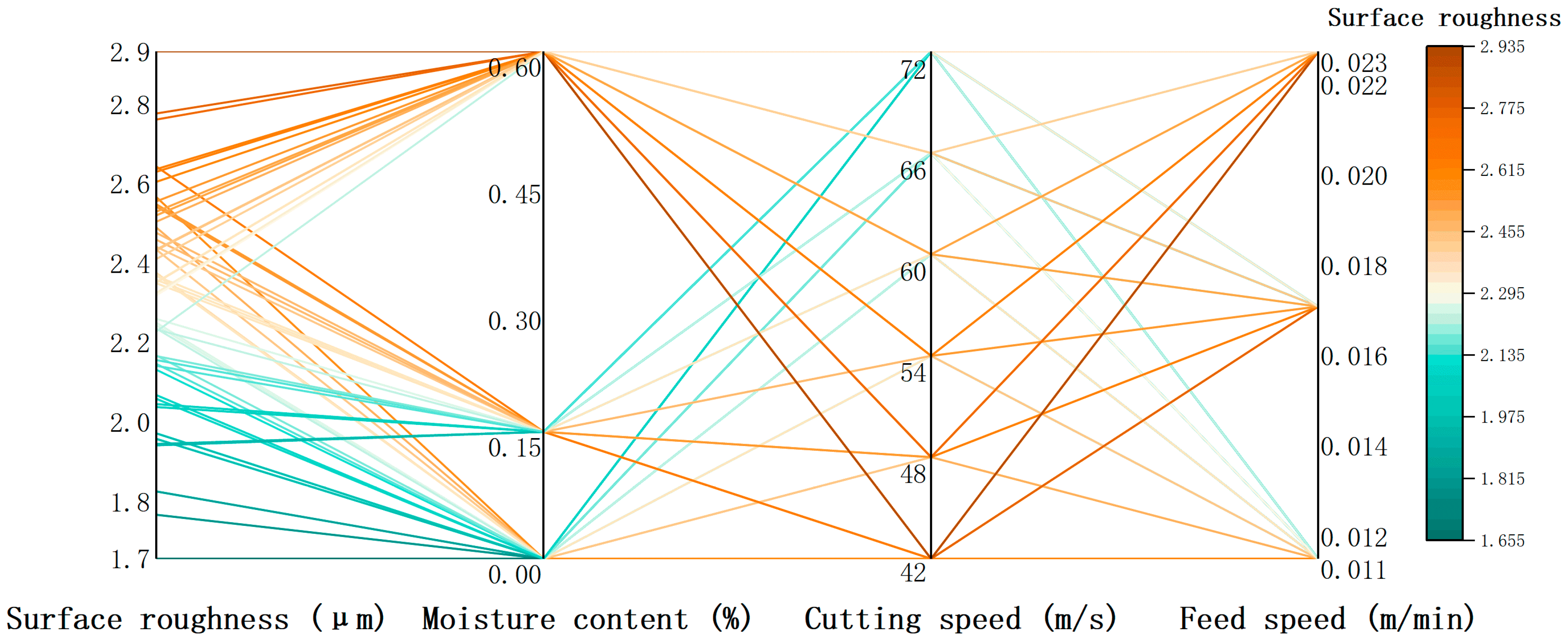
3. Results and Discussion

From the effects of moisture content, feed speed, and cutting speed on sawing surface roughness shown in Figure 5, it can be seen that the surface roughness decreases significantly with the increase in cutting speed. This effect is particularly pronounced at lower feed speeds (0.01128 m/min), where the change in roughness is more significant. As shown in Appendix A, Table A1, at 0% moisture content, when the cutting speed increases from 42.1497 m/s to 72.2566 m/s, the surface roughness decreases by 0.593 μm. This reduction is more notable compared to the feed speeds of 0.01686 m/min (0.517 μm) and 0.02250 m/min (0.507 μm), indicating that higher cutting speeds and lower feed speeds can effectively reduce the surface roughness of the machined material. Hanincová et al. reached similar experimental conclusions, pointing out that higher cutting speeds and lower feed rates effectively reduce the surface roughness after machining. This is primarily because high cutting speeds reduce the friction and heat accumulation between the tool and the workpiece while minimizing cutting force fluctuations and machining vibrations. Low feed rates, on the other hand, slow down tool wear and reduce the formation of surface ripples, thereby improving machining stability and achieving a smoother surface [4]. Additionally, taking the feed speed of 0.01686 m/min in Appendix A, Table A1 as an example, the rate of decrease in surface roughness is closely related to the moisture content. When the moisture content is 0%, the roughness decreases from 2.490 μm to 1.972 μm, showing the fastest reduction rate. When the moisture content is 15%, the roughness decreases from 2.548 μm to 1.945 μm, which is the second fastest rate. When the moisture content is 60%, the roughness decreases from 2.777 μm to 2.326 μm, showing the slowest reduction rate. This indicates that surface roughness increases with rising moisture content, while the rate of roughness change decreases as moisture content increases. Nascimento et al. also arrived at similar experimental conclusions, noting that surface roughness increases with higher moisture content because, at high moisture levels, the wood becomes softer. This causes the fibers to undergo plastic deformation and tearing more easily during the cutting process, resulting in increased surface unevenness. Furthermore, the change rate of roughness is inversely proportional to the moisture content, which may be because the impact of increased moisture content on cutting resistance gradually diminishes, thereby reducing roughness variations [6].

From the effects of moisture content, feed speed, and cutting speed on sawing power consumption shown in Figure 6, it can be observed that sawing power increases with higher wood moisture content and cutting speed. Taking the data for a feed speed of 0.01686 m/min in Appendix A, Table A1 as an example, when the moisture content increases from 0% to 60% and the cutting speed increases from 42.1497 m/s to 66.2352 m/s, the sawing power consumption rises from 0.344 kW to 0.411 kW. This indicates that higher moisture content and cutting speed leads to greater power consumption during the sawing process. In this regard, Hlásková et al. pointed out that sawing power increases with higher wood moisture content and cutting speed, mainly because high moisture content reduces the mechanical strength of the wood and increases cutting energy consumption. At the same time, increasing the cutting speed intensifies the friction between the tool and the wood, as well as heat build-up, further increasing power requirements. The combined effects of these factors result in a significant increase in cutting force and energy consumption [11].

As seen in Figure 7, sawing noise is influenced by both the cutting speed and the moisture content of the wood. The data show that the noise level increases gradually with the increase in water content and cutting speed. Taking the data of feed speed of 0.01686 m/min in Appendix A, Table A1 as an example, when the moisture content increases from 0% to 60% and the cutting speed increases from 42.1497 m/s to 66.2352 m/s, the noise level increases from 81.778 dB to 95.447 dB. This trend shows that high-speed processing of sawn timber with high moisture content produces higher noise levels. Owoyemi et al. obtained similar experimental conclusions. He pointed out that the increase in cutting speed and moisture content will significantly increase the mechanical noise level, mainly because the increase in cutting speed will enhance aerodynamic turbulence, intensify the contact force between the tool and the material, and cause the vibration and resonance of mechanical structures to amplify noise. Wood with a high moisture content, due to its increased flexibility and viscosity, produces greater friction and resistance during cutting, causing tool load fluctuations and unstable equipment operation, further increasing noise levels [13].

In order to obtain the minimum f(x), a preliminary analysis of the range of water content, cutting speed, and feed speed for the target combination shows that the effect of water content on sawing noise and power consumption is more significant. Although the power consumption and noise levels were relatively low at 0% moisture content, both changed significantly at 15% moisture content. A direct choice of 0% water content may lead to unstable predicted performance. In contrast, in the range of 15–60 percent water content, power consumption and noise do not change rapidly with changes in cutting speed, so it is more appropriate to select a water content range of 15–60 percent.

According to the data at a cutting speed of 66.2352 m/s in Appendix A, Table A1, it can be seen that as the feed speed increases from 0.01128 m/min to 0.01686 m/min, the sawing power increases slightly, while the sawing noise remains relatively unchanged. This is because the two feed speeds are already slow enough, resulting in insignificant changes in power consumption and noise during sawing at that feed speed. When the feed speed is further increased to 0.02250, an overall increase in sawing power and sawing noise occurs, with the mean value of sawing power increasing from 0.330 at the feed speed (0.01128–0.01686 m/min) to 0.371 and the mean value of sawing noise increasing from 93.609 to 94.330. Therefore, a lower feed speed interval of 0.01128–0.01686 should be selected m/min to balance the increase in power and noise within a certain range.

An increase in cutting speed is usually accompanied by an increase in noise and a decrease in sawing power. So, balancing the relationship between the two is the key to achieving the minimum f(x). As can be seen from the trend data in Figure 8, as the spindle speed increases gradually from a lower level (42.1497 m/s), the sawing power shows a decreasing trend, and the sawing noise shows a gradually increasing trend. By the high-speed cutting interval (66.2352–72.2566 m/s), the sawing power has been significantly reduced to a relatively stable low value, while the noise, despite a slight increase, is small and stays within the acceptable range. In addition, at higher cutting speeds, the surface roughness tends to a lower degree, which satisfies the requirement of f(x) on surface roughness to some extent. In contrast, the lower cutting speed range has a higher power consumption, although the noise is slightly lower; higher speeds further reduce the power, but the noise rises significantly. Therefore, combining the effects of cutting speed on power consumption, noise, and surface roughness, the cutting speed range of 66.2352–72.2566 m/s is selected as the best choice to achieve efficient and low-noise sawing.

Based on the above analysis, sawing power minimization requires higher cutting speeds but not too high, or else the noise will increase. Minimizing sawing noise requires lower cutting speeds and moderate feed speeds, and it is also necessary to work at moderate moisture content levels to avoid a sharp increase in noise.

By strictly controlling the model architecture and the way the dataset is divided, this paper uses the Transformer model along with the conventional PSO-BP model to simultaneously predict the sawing power consumption, surface roughness, and sawing noise, and analyze their respective performances, as shown in

Table 1. Performance comparison of standardized data.

	Iterations ↓		R2 ↑	MSE ↓	MAE ↓	RMSE ↓
Transformer	298	Power consumption	0.880	0.135	0.273	0.367
		Sawing noise	0.953	0.034	0.107	0.184
		Surface quality of sawn surfaces	0.977	0.059	0.177	0.243
PSO-BP	3000	Power consumption	0.871	0.210	0.293	0.458
		Sawing noise	0.870	0.111	0.304	0.333
		Surface quality of sawn surfaces	0.962	0.074	0.234	0.272

Note: “↑” indicates that the data closer to 1 is better, while “↓” indicates that the data closer to 0 is better.

.

The Transformer model better predicted sawing power consumption, mainly in terms of a higher R² value (0.880), indicating that the model explains more of the variability. In addition, the Transformer performs well in the three measures of error, MSE, MAE, and RMSE, which are 0.135, 0.273, and 0.367, respectively, which are lower than the corresponding measures of the PSO-BP model (0.210, 0.293, and 0.458), meaning that the Transformer model not only has higher accuracy in power prediction but also has less error; the error is also smaller.

The Transformer model also performs superiorly in the prediction of sawing noise. Its R² value is 0.953, which is much higher than the PSO-BP model’s, 0.870. This indicates that the Transformer is significantly better at capturing noise variations. Meanwhile, the MSE, MAE, and RMSE values of the Transformer model are 0.034, 0.107, and 0.184, respectively, while those of the PSO-BP model are 0.111, 0.304, and 0.333, and the Transformer is once again ahead of the curve in terms of noise prediction accuracy and error control.

For the prediction of saw-cut surface roughness, the Transformer model has a high R² value of 0.977, which almost perfectly predicts the change in surface roughness, compared to the PSO-BP model’s R² value of 0.962. Although the PSO-BP model also performs better in this metric, the Transformer’s MSE, MAE, and RMSE values (0.059, 0.177, and 0.243, respectively) are still significantly lower than those of the PSO-BP model (0.074, 0.234, and 0.272, respectively), which further proves the superiority of Transformer in predicting surface roughness.

In summary, the Transformer model predicts sawing power consumption, surface roughness, and sawing noise with higher accuracy and smaller errors, a significant advantage over the traditional PSO-BP model. Therefore, in the prediction task of the wood sawing process, the Transformer model shows excellent performance, which is worthy of further research and application.

This paper adopts the Transformer model based on Bayesian optimization to optimize the process parameters of wood sawing more accurately. The reliability and effectiveness of the optimization results are further verified by evaluating f(x) and Rate during the optimization process. As shown in Figure 9, Figure 9a shows the convergence of the objective function f(x), while Figure 9b shows the change in the convergence rate of the objective function f(x). The convergence graph of the objective function shows that in the initial optimization stage, the objective function value changes more dramatically because the optimization algorithm mainly explores the parameter space at this stage. However, as the iteration proceeds, the objective function value gradually stabilizes, indicating that the algorithm gradually enters the utilization stage, focusing on fine optimization in the known optimal area. Similarly, the convergence rate change graph of the objective function shows that as the optimization process proceeds, the objective function value gradually converges. In the first 20 iterations, the objective function value changes greatly, indicating that the optimization algorithm conducts a certain degree of global exploration at this stage. As the number of iterations increases, the objective function value tends to stabilize, which means that the optimal solution is gradually determined, and the optimization process converges successfully.

The final sawing optimization model obtained the best parameter combination of 24.7% water content of Pinus kesiya, 0.01638 m/min feed speed, and 67.8550 m/s cutting speed, which is in line with the above preliminary judgment based on the real data range. At this time, the corresponding power consumption is 0.232 kW, the sawing noise is 88.611 dB, and the surface roughness R_a is 2.606 μm.

Due to limitations in experimental conditions, it was not feasible to directly validate the predicted optimal sawing parameter combination. Therefore, a parameter combination close to the predicted values was selected for power consumption, sawing noise, and surface roughness predictions, followed by practical validation. The selected parameters were: wood moisture content of 24.7%, feed speed of 0.01632 m/min, and cutting speed of 67.4395 m/s. Under these conditions, the predicted results were a power consumption of 0.292 kW, sawing noise of 91.511 dB, and surface roughness (R_a) of 2.070 μm. In the actual sawing experiments, the measured results were a power consumption of 0.324 kW, sawing noise of 93.729 dB, and surface roughness (R_a) of 2.151 μm. As demonstrated by the sawing test, the actual measured power consumption, sawing noise, and surface roughness are somewhat different from those predicted by the optimal combination, and this difference may be due to several reasons.

Firstly, there is a certain difference between the best combination of parameters predicted by the model and the actual achievable parameters. Although the actual sawing parameters selected are close to the predicted best combination, small parameter differences may still have a large impact on the experimental results. For example, small changes in cutting speed and feed speed can significantly affect the friction and heat generated in the sawing process; thus, pre-experimental parameters may affect the changes in energy consumption and noise.

Secondly, the model is trained based on a certain amount of experimental data during the building process, so its predictive ability is valid within a certain range. However, the complexity and variability of the actual test conditions may exceed the predictive range of the model, leading to differences between the experimental and predicted results.

Nonetheless, the general trend of the model predictions coincides with the actual experimental results. The power consumption and surface roughness under the actual operating conditions are close to the results predicted by the model, indicating that the model has good practicality and guiding value.

4. Conclusions

In this paper, by constructing a sawing prediction model for Pinus kesiya based on the Transformer model and combining it with the Bayesian optimization method, the sawing parameters were successfully optimized according to the required objective function, enhancing the sawing process’s performance. In the prediction of sawing power consumption, sawing surface roughness and sawing noise, the Transformer model demonstrated significant advantages over the traditional PSO-BP model, manifested in higher prediction accuracy and smaller error. In addition, the optimization method of sawing parameters based on Bayesian optimization proposed in this paper also shows good convergence and practicability in experimental validation and can find parameter combinations close to the actual optimum.

Future research could validate the generalizability of this framework on multiple wood types and introduce more complex pre-experimental parameters, such as tool wear and temperature variations, to enhance the model’s applicability. Meanwhile, developing an adaptive sawing system based on real-time data inputs and comparing the performance of other intelligent algorithms, such as deep reinforcement learning and LSTM networks, will further improve the optimization. Further optimizing the sawing parameters is expected to reduce the energy consumption and carbon footprint and provide a more forward-looking reference for green production in the wood industry.

These research results provide a clear direction and feasibility for future academic discussions and industrial applications and open up a new technical way for sawing process optimization.

References

1. e Silva, J.C.; Graudal, L. Evaluation of an international series of Pinus kesiya provenance trials for growth and wood quality traits. For. Ecol. Manag. 2008, 255, 3477–3488. [Google Scholar] [CrossRef]
2. Orlowski, K.A.; Ochrymiuk, T.; Hlaskova, L.; Chuchala, D.; Kopecky, Z. Revisiting the estimation of cutting power with different energetic methods while sawing soft and hard woods on the circular sawing machine: A Central European case. Wood Sci. Technol. 2020, 54, 457–477. [Google Scholar] [CrossRef]
3. Gholamiyan, H.; Gholampoor, B.; Tichi, A.H. Effects of Cutting Parameters on the Sound Level and Surface Quality of Sawn Wood. BioResources 2022, 17, 1397. [Google Scholar] [CrossRef]
4. Hanincová, L.; Procházka, J.; Novák, V.; Kopecký, Z. Influence of moisture content on cutting parameters and fracture characteristics of spruce and Oak wood. Drv. Ind. 2022, 73, 341–349. [Google Scholar] [CrossRef]
5. Gao, Y.; Wang, Y.; Qu, A.; Kan, J.; Kang, F.; Wang, Y. Study of sawing parameters for caragana korshinskii (ck) Branches. Forests 2022, 13, 327. [Google Scholar] [CrossRef]
6. Nascimento, D.F.R.; Melo, L.D.L.; Silva, J.D.; Trugilho, P.F.; Napoli, A. Effect of moisture content on specific cutting energy consumption in Corymbia citriodora and Eucalyptus urophylla woods. Scientia Forestalis 2017, 45, 221–227. [Google Scholar] [CrossRef]
7. Fekiač, J.; Svoreň, J.; Gáborík, J.; Němec, M. Reducing the energy consumption of circular saws in the cutting process of plywood. Coatings 2022, 12, 55. [Google Scholar] [CrossRef]
8. Svoreň, J.; Naščák, Ľ.; Barcík, Š.; Koleda, P.; Stehlík, Š. Influence of circular saw blade design on reducing energy consumption of a circular saw in the cutting process. Appl. Sci. 2022, 12, 1276. [Google Scholar] [CrossRef]
9. Çakıroğlu, E.O.; Demir, A.; Aydın, İ.; Büyüksarı, Ü. Prediction of optimum CNC cutting conditions using artificial neural network models for the best wood surface quality, low energy consumption, and time savings. BioResources 2022, 17, 2501. [Google Scholar] [CrossRef]
10. Cakmak, A.; Malkocoglu, A.; Ozsahin, S. Optimization of wood machining parameters using artificial neural network in CNC router. Mater. Sci. Technol. 2023, 39, 1728–1744. [Google Scholar] [CrossRef]
11. Hlásková, L.; Kopecký, Z.; Novák, V. Influence of wood modification on cutting force, specific cutting resistance and fracture parameters during the sawing process using circular sawing machine. Eur. J. Wood Wood Prod. 2020, 78, 1173–1182. [Google Scholar] [CrossRef]
12. Pangestu, K.T.P.; Nandika, D.; Wahyudi, I.; Usuki, H.; Darmawan, W. Innovation of helical cutting tool edge for eco-friendly milling of wood-based materials. Wood Mater. Sci. Eng. 2022, 17, 607–616. [Google Scholar] [CrossRef]
13. Owoyemi, M.J.; Falemara, B.; Owoyemi, A.J. Noise pollution and control in wood mechanical processing wood industries. Preprints 2016. [CrossRef]
14. Das, S.; Roy, R.; Chattopadhyay, A.B. Evaluation of wear of turning carbide inserts using neural networks. Int. J. Mach. Tools Manuf. 1996, 36, 789–797. [Google Scholar] [CrossRef]
15. Cus, F.; Zuperl, U. Approach to optimization of cutting conditions by using artificial neural networks. J. Mater. Process. Technol. 2006, 173, 281–290. [Google Scholar] [CrossRef]
16. Gu, P.; Zhu, C.M.; Wu, Y.Y.; Mura, A. Energy consumption prediction model of SiCp/Al composite in grinding based on PSO-BP neural network. In Solid State Phenomena; Trans Tech Publications Ltd.: Wollerau, Switzerland, 2020. [Google Scholar]
17. Hadad, M.; Attarsharghi, S.; Abyaneh, M.D.; Narimani, P.; Makarian, J.; Saberi, A.; Alinaghizadeh, A. Exploring New Parameters to Advance Surface Roughness Prediction in Grinding Processes for the Enhancement of Automated Machining. J. Manuf. Mater. Process. 2024, 8, 41. [Google Scholar] [CrossRef]
18. Wei, W.; Shang, Y.; Peng, Y.; Cong, R. Prediction Model of Sound Signal in High-Speed Milling of Wood–Plastic Composites. Materials 2022, 15, 3838. [Google Scholar] [CrossRef]
19. Das, H.; Jena, A.K.; Nayak, J.; Naik, B.; Behera, H.S. A novel PSO based back propagation learning-MLP (PSO-BP-MLP) for classification. In Computational Intelligence in Data Mining-Volume 2: Proceedings of the International Conference on CIDM, 20–21 December 2014; Springer: Berlin/Heidelberg, Germany, 2015. [Google Scholar]
20. Chenglei, H.; Kangji, L.; Guohai, L.; Lei, P. Forecasting building energy consumption based on hybrid PSO-ANN prediction model. In Proceedings of the 2015 34th Chinese Control Conference (CCC), Hangzhou, China, 28–30 July 2015; IEEE: Piscataway, NJ, USA, 2015. [Google Scholar]
21. Ahmed, S.; Nielsen, I.E.; Tripathi, A.; Siddiqui, S.; Ramachandran, R.P.; Rasool, G. Transformers in time-series analysis: A tutorial. Circuits Syst Signal Process. 2023, 42, 7433–7466. [Google Scholar] [CrossRef]
22. Choi, S.R.; Lee, M. Transformer architecture and attention mechanisms in genome data analysis: A comprehensive review. Biology 2023, 12, 1033. [Google Scholar] [CrossRef]
23. Cao, K.; Zhang, T.; Huang, J. Advanced hybrid LSTM-transformer architecture for real-time multi-task prediction in engineering systems. Sci. Rep. 2024, 14, 4890. [Google Scholar] [CrossRef]
24. Jiang, L.; Jiang, C.; Yu, X.; Fu, R.; Jin, S.; Liu, X. DeepTTA: A transformer-based model for predicting cancer drug response. Brief. Bioinform. 2022, 23, bbac100. [Google Scholar] [CrossRef] [PubMed]
25. Rahman, A.U.; Alsenani, Y.; Zafar, A.; Ullah, K.; Rabie, K.; Shongwe, T. Enhancing heart disease prediction using a self-attention-based transformer model. Sci. Rep. 2024, 14, 514. [Google Scholar] [CrossRef] [PubMed]
26. Kim, D.-K.; Kim, K. A convolutional transformer model for multivariate time series prediction. IEEE Access 2022, 10, 101319–101329. [Google Scholar] [CrossRef]
27. Teischinger, A.; Avramidis, S.; Hansmann, C. Sawn Timber Steaming and Drying. In Springer Handbook of Wood Science and Technology; Springer: Berlin/Heidelberg, Germany, 2023; pp. 1167–1210. [Google Scholar]
28. Dietsch, P.; Franke, S.; Franke, B.; Gamper, A.; Winter, S. Methods to determine wood moisture content and their applicability in monitoring concepts. J. Civ. Struct. Health Monit. 2015, 5, 115–127. [Google Scholar] [CrossRef]
29. Chuchala, D.; Orlowski, K.A.; Hiziroglu, S.; Wilmanska, A.; Pradlik, A.; Mietka, K. Analysis of surface roughness of chemically impregnated Scots pine processed using frame-sawing machine. Wood Mater. Sci. Eng. 2023, 18, 1809–1815. [Google Scholar] [CrossRef]
30. Glass, S.V.; Boardman, C.R.; Thybring, E.E.; Zelinka, S.L. Quantifying and reducing errors in equilibrium moisture content measurements with dynamic vapor sorption (DVS) experiments. Wood Sci. Technol. 2018, 52, 909–927. [Google Scholar] [CrossRef]
31. Demir, A.; Cakiroglu, E.O.; Aydin, I. Determination of CNC processing parameters for the best wood surface quality via artificial neural network. Wood Mater. Sci. Eng. 2022, 17, 685–692. [Google Scholar] [CrossRef]
32. DIN 4768 (1990); Determination of Values of Surface Roughness Parameters Ra, Rz, Rmax Using Electrical Contact (Stylus) Instruments, Concepts and Measuring Conditions. Deutsches Institut für Norming: Berlin, Germany, 1990.
33. Licow, R.; Chuchala, D.; Deja, M.; Orlowski, K.A.; Taube, P. Effect of pine impregnation and feed speed on sound level and cutting power in wood sawing. For. Ecol. Manag. 2020, 272, 122833. [Google Scholar] [CrossRef]
Figure 1. Sawing test bench: (a) main view of sawing test bench, (b) schematic diagram of the sawing position and sawtooth rake angle of the sample to be cut.
Forests 15 02144 g001
Figure 2. Configuration of the surface roughness measurement on the sample.
Forests 15 02144 g002
Figure 3. Saw cut prediction modeling framework.
Forests 15 02144 g003
Figure 4. Flowchart of the sawing optimization model.
Forests 15 02144 g004
Figure 5. Parallel coordinates plot. Effects of moisture content, cutting speed, and feed rate on surface roughness.
Forests 15 02144 g005
Figure 6. Parallel coordinates plot. Effects of moisture content, cutting speed, and feed rate on sawing power.
Forests 15 02144 g006
Figure 7. Parallel coordinates plot. Effects of moisture content, cutting speed, and feed rate on sawing noise.
Forests 15 02144 g007
Figure 8. Trend of sawing power and noise against cutting speed.
Forests 15 02144 g008
Figure 9. Convergence analysis of sawing optimization model. (a) Objective function convergence analysis, (b) analysis of the change of objective function convergence rate.
Forests 15 02144 g009