Article

Relative Humidity Dominances in Negative Air Ion Concentration: Insights from One–Year Measurements of Urban Forests and Natural Forests

School of Ecology and Nature Conservation, Beijing Forestry University, Beijing 100083, China
*
Author to whom correspondence should be addressed.
These authors contributed equally to this work.
Forests 2024, 15(2), 295; https://doi.org/10.3390/f15020295
Submission received: 15 December 2023 / Revised: 24 January 2024 / Accepted: 30 January 2024 / Published: 3 February 2024
(This article belongs to the Section Forest Meteorology and Climate Change)

Abstract

:
Forests are one of the most important sources of negative oxygen ions (NAIs). NAIs have been recognized as beneficial for both physical and mental well–being, and higher concentrations of NAIs have been associated with improved health. However, the environmental factors that predominantly influence NAI concentration and their relationship with NAIs remain uncertain. This study aims to investigate the dominant factors and their impact on NAI concentration by observing NAIs and various environmental factors in two different environments (natural forest and urban forest) in the Beijing region over a one–year period. Through our investigation, we aimed to identify the key factor as well as other influential variables affecting NAI concentration. Our analysis encompassed the examination of dynamic concentration changes over multiple time scales, revealing uniform trends in both forest types. Notably, natural forests consistently demonstrated higher NAI concentration across these time scales, attributable to greater vegetation density and the stability of the forest microenvironment. By utilizing regression, correlation analysis, and structural equation analysis, we determined that relative humidity (RH) has the most significant effect on NAI concentration. Notably, both NAI concentration and RH displayed similar patterns across multiple time scales. When considering hourly average daily variation, the lowest values for both NAI concentration and RH were observed at noon, followed by an increase that persisted throughout the night. Seasonal average variation showed that both NAI concentration and RH peaked in the summer, followed by autumn. In terms of daily average annual variation, summer exhibited more days with high NAI concentration and high RH, which can be attributed to the increased rainfall during that season. Rainy weather was found to contribute to higher NAI concentration and RH levels. Furthermore, our findings revealed that on a daily scale, high RH and high NAI concentration occurred more frequently under conditions of high air temperature and low wind speed. However, the air quality index demonstrated only a minor effect in urban forest, while net radiation exhibited no significant influence on NAI concentration and RH. The fitted equations and trends of the aforementioned environmental factors with NAI concentration and RH were found to be comparable. The path analysis further corroborates these conclusions. The findings of this study indicate that RH is the primary factor driving the fluctuations in NAI concentration across various time scales, including hourly, daily, and seasonal variations. The study revealed that wind speed indirectly impacts NAI concentration by modulating RH. In contrast, air temperature influences NAI concentration both indirectly through RH and directly. The environmental factors affecting NAI concentration in the two types of forests are similar, but the degrees vary; in urban forests, wind speed, air quality index, and RH are slightly higher, while in natural forests, air temperature is slightly higher. This discovery further enhances our understanding of the underlying mechanisms and dynamic changes in NAI concentration within urban forests and natural forests. Moreover, it confirms the reliability and effectiveness of using RH as an indicator to monitor changes in NAI concentration over time.

1. Introduction

Forests can ionize the surrounding air and release free electrons, which combine with oxygen molecules to form negative air ions. Negative oxygen ions (NAIs) are individual molecules or light ion clusters that carry a negative charge in the atmosphere [1]. They are specifically called negative oxygen ions due to oxygen’s exceptional ability to capture free electrons and its inherent inclination to acquire them [1,2]. NAIs offer various psychological and physiological benefits to the human body, including stress reduction [3], enhancement of cardiovascular function [4], and improvement of cognitive abilities [5]. Animal experiments [6,7] and human studies investigating both physiological and psychological health [3,8] have confirmed NAIs’ effectiveness as supplementary treatment methods for a wide range of diseases. Furthermore, NAIs contribute to air purification and dust adsorption, playing a crucial role in maintaining environmental cleanliness levels [9,10,11]. The process of urbanization has given rise to new challenges, such as urban pollution and ecological degradation, which have raised concerns regarding the health advantages of urban areas and their surrounding natural environment. Consequently, the concentration of NAIs has emerged as a critical indicator for evaluating air quality and associated health benefits and it has become a prominent topic in the field of atmospheric research.
The sources and influencing factors of NAIs are intricate and variable, constrained by environmental factors such as climatic conditions [12], vegetation types [11], and geographical conditions [13,14]. NAIs can derive from diverse natural electrical phenomena including lightning, thunderstorms, and plant leaf tips [15,16]. Additionally, they may result from radiation [17], the shearing forces of water [18], and the photoelectric effect of plant photosynthesis [19,20]. Numerous studies have underscored variations in the dynamic analysis of NAI concentration, revealing either double–peak or single–peak curves of daily fluctuation patterns. The double–peak curve signifies that the highest values occur during the morning and afternoon, while the lowest values are observed at noon and night [1,21]. In contrast, the single–peak curve exhibits the highest peak in the morning [22]. Seasonally, it has been observed that NAIs exhibit higher concentration during summer compared to autumn and winter [21].
To enhance the understanding of current research on the determinants of NAI concentration, we have compiled Table 1, which summarizes the key influencing factors. This study encompasses a diverse range of environmental settings, spanning climates from humid to semi–humid and from temperate to subtropical, primarily focusing on research conducted in the last five years. The examined factors include meteorological elements (including relative humidity (RH), air temperature (TA), wind speed (WS), etc.), pollutants (such as PM2.5, NOx, SO2, etc.), and vegetation structure (plant communities, canopy density, etc.), among others. The dominant factors influencing NAI concentration remain to be conclusively determined. Among meteorological elements, RH has been most frequently noted as a significant factor, followed by TA and WS. Additionally, factors including PM2.5, canopy density, and altitude are consistently acknowledged as pivotal. A year–long study conducted by Luo et al. kept track of the NAI concentrations and various environmental factors in urban parks in Shanghai. Their findings suggested that the “water factor”, predominantly controlled by RH, had the most significant positive effect on NAI concentration [23]. Water molecules in the atmosphere contribute to the synthesis of NAIs, playing a role in reducing airborne particulate matter and thereby indirectly prolonging the lifespan of NAIs. Furthermore, Li et al. conducted a study on the effect of atmospheric pollutants on the NAI concentration in the forest environment of Wuyishan National Park. This study reveals PM2.5 has a significant negative impact on the NAI concentration [1]. Particulate matter carries a positive charge and persists in the atmosphere, combining with NAIs to form substantial molecular sediment [24,25].
The production and degradation of NAIs is intricate, and the relationship between NAI concentration and environmental factors remains elusive. Prior research has utilized portable devices for measuring NAI concentration; however, this approach is constrained by several limitations, such as data collection being confined to daytime hours, a dependence on limited sample sizes, low accuracy, and poor consistency, which compromises the reliability and scalability of the findings. There is a noticeable variance in the vegetation characteristics and microclimates between urban and natural forests. Comparative analyses of these forest types are crucial for evaluating their respective health impacts regarding the release of NAIs. Historically, studies have predominantly focused on a single forest type, resulting in a gap in comparative research between urban and natural forests. To address these shortcomings, our study employed fixed monitoring systems, enabling the measurement of NAI concentration and environmental factors in two distinct settings: an urban forest and a natural forest. The objectives of this study are twofold: (1) to explore the relationship between NAI concentration and environmental factors in both urban and natural forests, identifying the dominant influencing factors, and (2) to ascertain the temporal dynamics of NAI concentration within these forest types. This study conducts a quantitative analysis of meteorological factors and pollutants while excluding other variables such as topography and vegetation characteristics. Fulfilling these objectives will enhance decision–makers’ understanding of the factors driving NAI production in different forest ecosystems.

2. Materials and Methods

2.1. Study Area

Long–term, fixed monitoring of NAI concentration and environmental factors was conducted at both locations over a one–year period. The study was conducted at two distinct locations, namely Baihuashan National Nature Reserve (Mentougou District, Beijing, China; altitude: 1142 m; coordinates: 115°33′59″ E, 39°49′58″ N) and Qinglonghu Forest Park (Fangshan District, Beijing, China; altitude: 103 m; coordinates: 116°26′57″ E, 39°46′43″ N) (Figure 1). The abbreviations BHS and QLH denote the Baihuashan and Qinglonghu sites, respectively. Both sites exhibit a typically northern temperate semi–humid continental monsoon climate, characterized by hot and rainy summers, cold and dry winters, and short transitional seasons with the majority of rainfall occurring between June and August. The BHS site encompasses a natural secondary forest primarily composed of larch trees, with a canopy height varying between 8 to 15 m and notable canopy coverage. The understory is distinguished by abundant vegetation and is relatively undisturbed by human activities. Conversely, the QLH site predominantly consists of urban mixed forests characterized by shorter canopies and a diverse array of coniferous and broad–leaved species such as black locust, wax tree, and turpentine. Additionally, the region encompasses grasslands, shrubberies, and walking trails and is encircled by urban development zones with significant human activity.

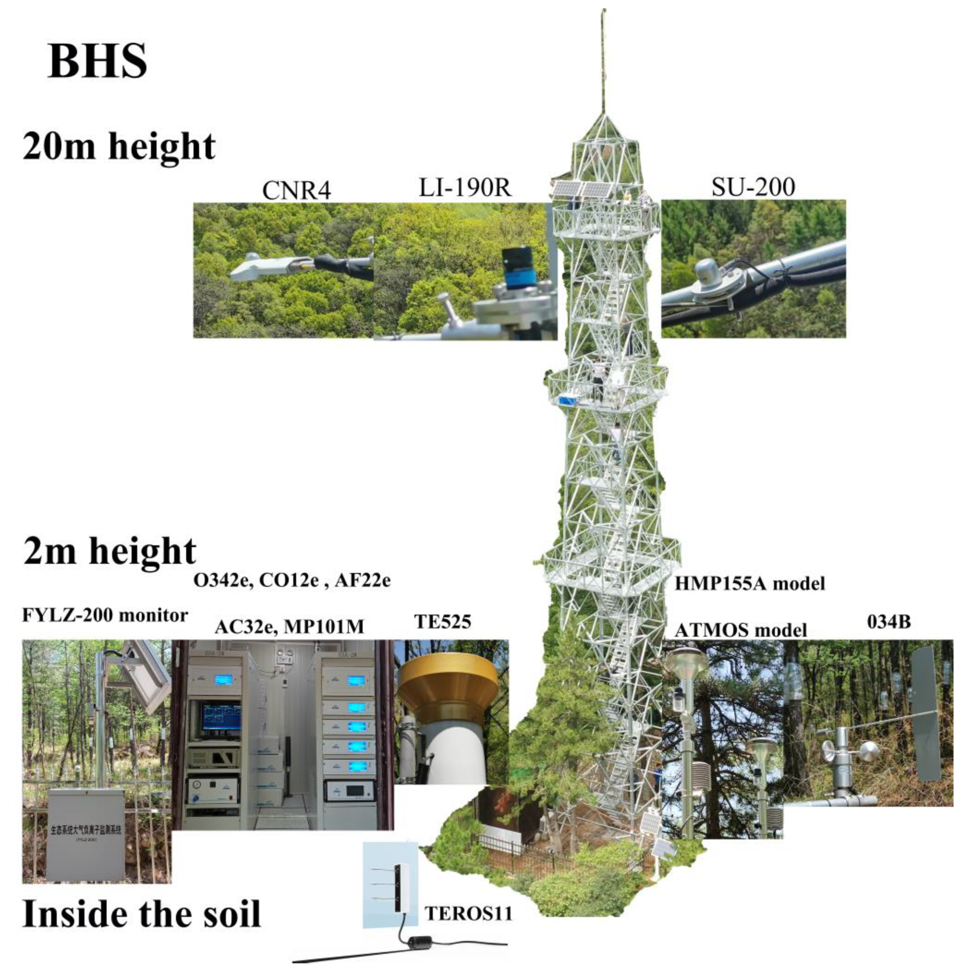
2.2. Observation Instrument

A series of environmental factor data and NAI concentration data was measured in two forest environments through fixed monitoring instruments. The environmental factors described in this study include meteorological factors, radiation factors, soil factors, and air quality factors. The specific environmental factors are listed in Table 2.The FYLZ–200 negative oxygen ion monitor (Sunshine Weather, Jinzhou, China), features an ion mobility of equal to or greater than 0.4 cm2/V·s, with a sampling frequency of 1 min. For monitoring purposes, this probe was positioned at a height of 1.8 m above ground level, approximating the average respiratory height of humans. The monitoring equipment for meteorological factors and air/pollutants was positioned at a height of 2 m near the monitoring tower. The devices measuring radiation factors were installed at approximately 20 m on the tower, while those for soil factors were situated underground. An illustration of the equipment installation, using the BHS site as an example, can be found in Figure A1.

2.3. Data Analysis

In this study, the raw resolution data were averaged over a one–hour interval. To guarantee data integrity and reliability, comprehensive filtering and cleaning were performed on the processed data using R 4.1. We did not utilize any specific R packages but employed R’s fundamental data processing capabilities, including loop structures and conditional judgments [39]. The key steps are as follows: 1. Outlier Screening: Each data point is compared with its preceding value. If the current value is more than five times or less than one–fifth of the preceding value, it is considered an outlier and marked as missing (NA). 2. Identification of Continuous Repetitive Values: We identify sequences of six or more consecutive identical data points as abnormal values and label them as NA. 3. Handling of Small Values: For data points with values less than 10, we calculate the average of the two data points before and after, round it off, and record it as the value at that time. 4. Secondary Screening: After reassigning values, if the value still falls below 10, it is omitted and reported as NA. The complete process was applied to screen the NAI concentration data, while the initial step was used to screen the environmental factors data. Throughout the study, 7145 data sets were collected in BHS, while 8413 data sets were obtained in QLH. Following the aggregation of daily average data, the resultant yearly observations were categorized based on meteorological seasons: spring observation data spanned from March to May, summer observation data encompassed June to August, autumn observation data covered September to November, and winter observation data ranged from December to February. For the purpose of investigating the impact of solar radiation, we opted for a daytime monitoring interval from 8:00 to 17:00 and a nighttime monitoring interval from 22:00 to 4:00, deliberately enhancing the illumination contrast between these periods.
In our study, we initially identified significant environmental factors using Pearson correlation analysis, followed by a multivariate linear regression analysis employing the stepwise method in SPSS 26. This method systematically selects influential independent variables and eliminates non–significant ones, aiming to construct an optimal regression model. The process continues until no additional variables can be included or excluded. The magnitude of the Beta values in the standardized factors indicates the importance of each environmental factor.
Integrating the results of correlation and linear regression analyses, potential key environmental factors were identified. Subsequently, scatter plots and path analysis were employed to further determine the important environmental factors for NAI concentration. These scatter plots are based on R2 values to assess the extent of influence, with R2 indicating the explanatory power of the model. A higher R2 value suggests a stronger correlation and explanatory capacity within the model. The fit indices used in Structural Equation analysis include the Adjusted Goodness of Fit Index (AGFI), Root Mean Square Error of Approximation (RMSEA), and Comparative Fit Index (CFI). AGFI assesses the model fit, with good fit indicated by values close to 1, and a preferable threshold above 0.90. RMSEA measures the model’s approximation to the data; it is ideally less than 0.05, but values below 0.08 are also acceptable. CFI compares the actual model to an ideal model, with values closer to 1 indicating a better fit, and values above 0.90 typically indicating a good fit. These indices help us evaluate the accuracy and reliability of our model in assessing the impact of environmental factors on NAI concentration. In addition to the aforementioned fit coefficients, path analysis diagrams utilize standardized regression coefficients, measurement errors, and covariances to depict relationships between variables. Values on paths (indicated by solid lines) represent standardized regression coefficients, gauging the impact strength of one variable on another. The magnitude and direction of these coefficients indicate the strength and nature of relationships between variables, with values closer to 1 or −1 denoting stronger relationships and those near 0 indicating weaker ones. Values on circular icons represent measurement error, which refers to the portion of the observed variable not fully explained by related factors. Smaller errors indicate greater accuracy of the model in capturing data patterns. Values on dashed lines represent covariances, quantitatively reflecting the correlation magnitude between paired variables.

3. Results

3.1. Relationship between NAI Concentration and Environmental Factors

3.1.1. Pearson Correlation Analysis

Daily mean data were utilized to calculate Pearson’s correlation between environmental factors and NAI concentration. The results, presented in Table 3, show a noteworthy positive correlation between RH and NAI concentration. The correlation coefficients for BHS and QLH were 0.967 (p < 0.000) and 0.978 (p < 0.000), respectively. Various environmental factors exhibited correlations with NAI concentration, and some distinctions were observed between the two study sites. In both locations, TA, SWC, RN, TS, and Prec. demonstrated positive correlations with NAI concentration. Conversely, PA, UVA, and WS exhibited negative correlations with NAI concentration. Pollutants displayed correlations with NAI concentration, though their correlation coefficients were predominantly weak or statistically insignificant.

3.1.2. Multivariate Linear Regression Analysis

We conducted linear regression analysis on the environmental factors significantly associated with NAI concentration. Table 4 shows the best regression models with R2 values of 0.968 and 0.973, demonstrating the effectiveness and high explanatory power of the models. Among the environmental factors, RH exhibited considerably higher beta values of 0.897 and 0.930 in both regions compared to other variables. These findings suggested that RH played a central role in NAI concentration at both sites. In addition, prec. positively influenced NAI concentration in both regions, while RN and pollutants (NO, NOX, SO2) had a negative impact. There were disparities in the results of some environmental factors between the two sites. TA had a Beta value of 0.316 at the QLH site and it was excluded from the regression model at the BHS site due to its insignificance (p > 0.05). TS exhibited varying effects on NAI concentration in the BHS and QLH sites. This divergence could be attributed to the environmental distinctions between natural forests and urban forests.

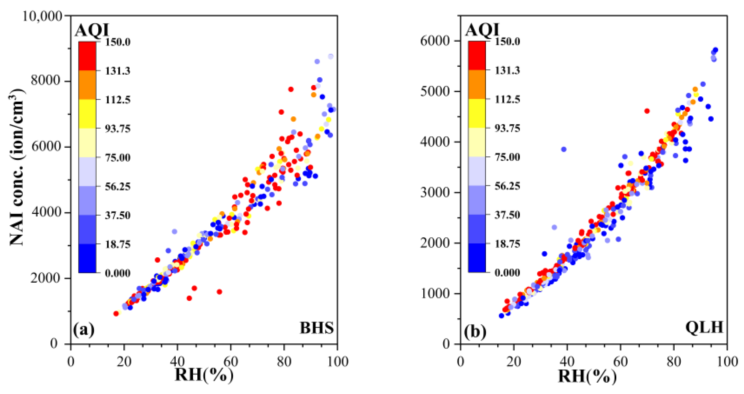
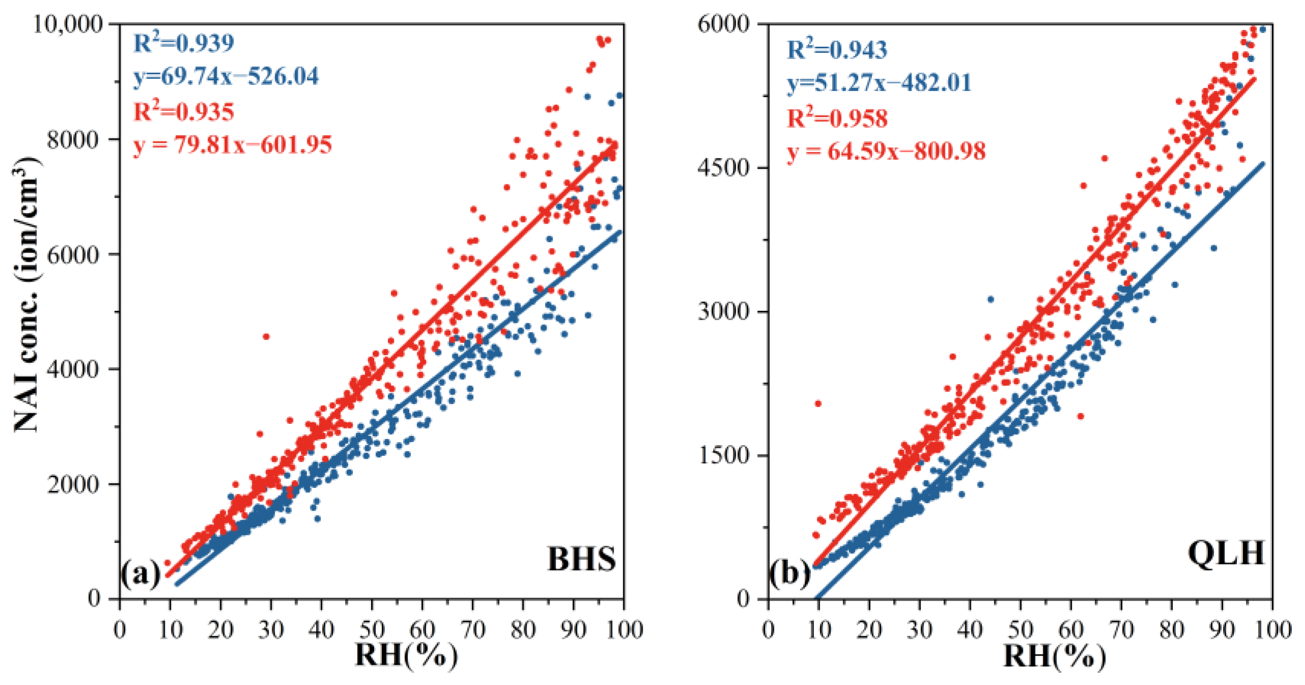
3.1.3. The Relationship between NAI Concentration and RH

Through Pearson correlation analysis and multiple linear regression analysis, it can be concluded that RH emerges as the most influential factor impacting NAI concentration. The segmented correlation between NAI concentration and RH is illustrated in Figure 2. The R2 values, indicative of the strength of the correlation, are presented with daytime data in blue and nighttime data in red. Notably, we observed a steeper slope in NAI concentration during nighttime compared to daytime, suggesting that RH exerts a more pronounced influence during the night. The R2 values for both daytime and nighttime at both sites exceeded 0.93, indicating that RH stands as the predominant factor shaping NAI concentration throughout the day, although it may play a stronger role at night.

3.2. Temporal Dynamics of NAI Concentration and RH

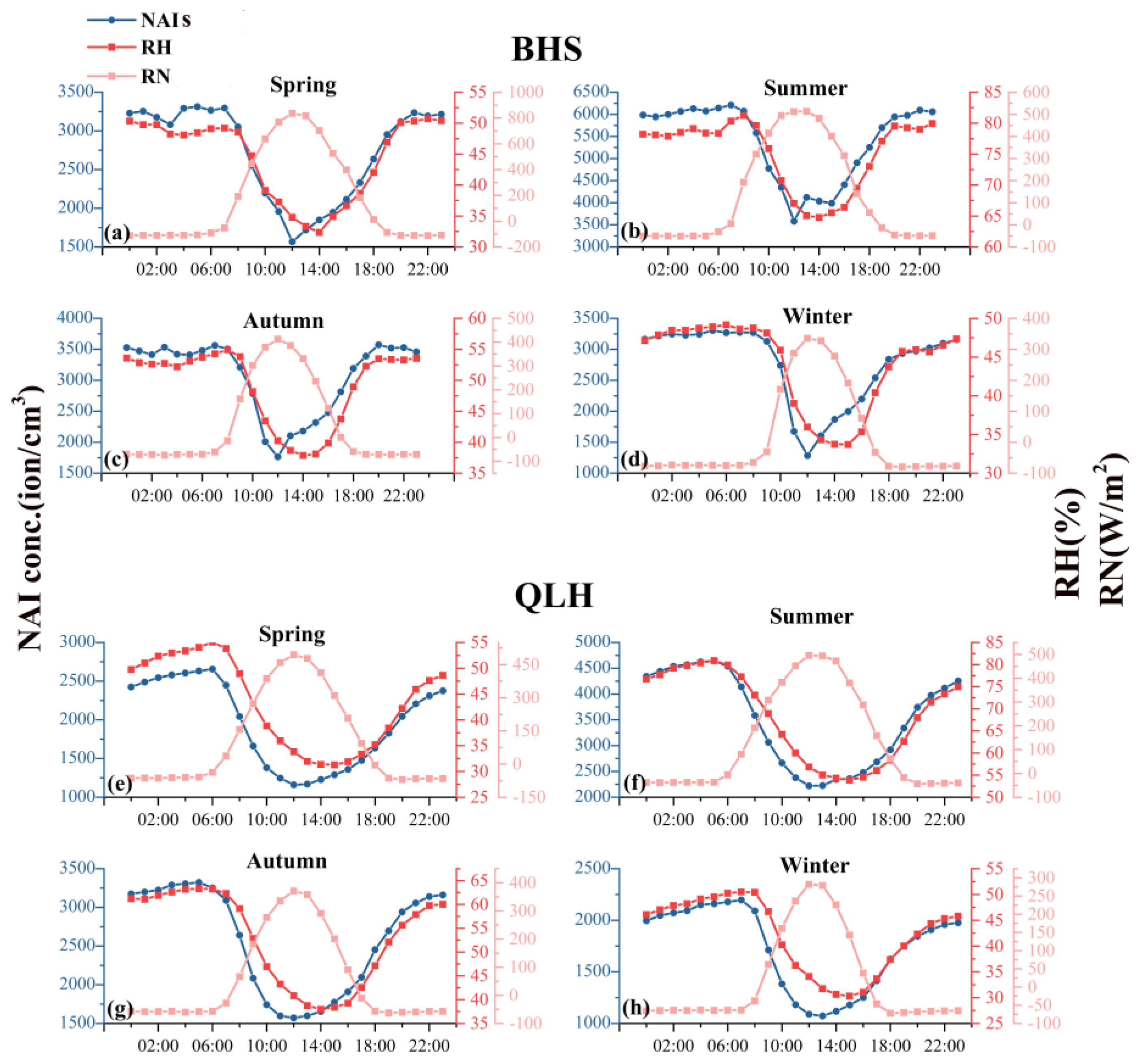
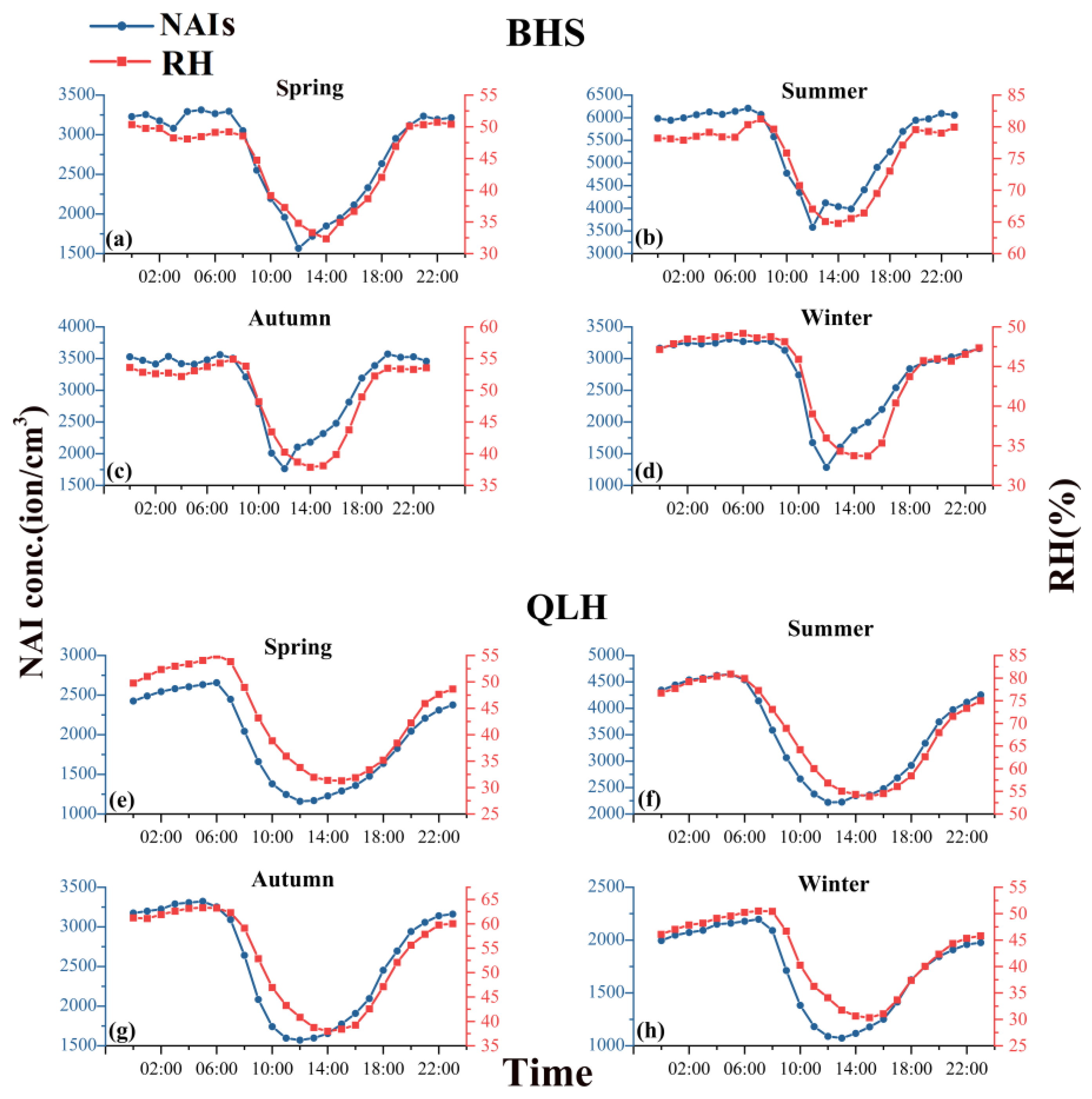
3.2.1. Seasonal Diurnal Variations in Hourly Averages

Figure 3 illustrates the diurnal variations in RH and NAI concentration. Consistent patterns were discerned across both sites throughout the four seasons, showcasing the nadirs of NAI concentration and RH during midday and their zeniths during the night. At approximately 12:00, the NAI concentration reached its minimum, while RH levels bottomed out around 14:00 or 15:00 before initiating an ascent. After the termination of the nightly peak period, the decline timings diverged between the BHS and QLH sites. At BHS, both NAI concentration and RH decreased around 8:00 a.m., whereas at QLH, the decline occurred around 6:00 a.m. In Figure A2, the daily variation of RN is added, revealing an inverse relationship with the changes in RH and NAIs. The inflection points of these changes are nearly identical. Seasonal shifts lead to variations in RN trends, such as a later increase in RN during winter, yet the turning points of all three variables remain similar across different seasons.

3.2.2. Seasonal Variations in Average Values

Figure 4 shows seasonal variations in NAI concentration and RH, with summer exhibiting the highest values, followed by autumn, spring, and winter. The NAI concentration was consistently higher during seasons with elevated RH levels. Across all seasons, BHS consistently exhibited a higher NAI concentration compared to QLH, although the difference in RH between the two sites was insignificant.

3.2.3. Annual Variations in Daily Averages

Figure 5 illustrates the annual fluctuations in the daily average levels of NAI concentration and RH at both the BHS and the QLH sites. Our study revealed a consistent annual pattern, characterized by elevated RH and NAI concentration from mid–June to late August. This pattern substantiates a notably positive correlation between RH and NAI concentration, demonstrating synchronous variation trends. On days with high RH, NAI concentration demonstrated an increase. Both RH and NAI concentration exhibited substantial variability between consecutive days and displayed a positive correlation. The substantial increase in NAI concentration during June, July, and August in Beijing can be attributed to intense rainfall, which led to a sharp rise in RH. The concurrent high levels of NAI concentration and RH are likely linked to the pronounced rainfall intensity.

3.3. Effect of Individual Factors on the NAI Concentration and RH

3.3.1. Correlation Analysis of the NAI Concentration and RH under Different TA Conditions

This study investigated the correlation between NAI concentration and RH at different temperature levels. According to Figure 6, the low–temperature points are primarily located in the lower curve range, which means that when the RH was the same, the NAI value was lower than that in the high–temperature point. The results indicate that the NAIs were higher under high–temperature conditions. Figure 7 presents the correlations and R2 values among TA, NAIs, RH, and WVD, highlighting the statistical interrelationships between these environmental parameters. The scatter plot analyses of NAIs, RH, and TA reveal higher R2 values at the BHS site compared to those at the QLH site. Specifically, for NAI concentration and RH relative to TA at the BHS site, the R2 values are 0.228 and 0.180, respectively. In contrast, at the QLH site, the R2 values for NAI concentration and RH against TA are 0.186 and 0.124, respectively. Using fitting equations to ascertain the peaks, it was observed that the TA is 1 °C when the scatter plot fitting line of the NAI concentration and the RH reached its maximum level at the BHS site. Conversely, at the QLH site, the TA values were found to be −7.8 °C and −31 °C, respectively. The scatter plots incorporating WVD against TA demonstrate a distinct trend: WVD increases as TA rises, with an accelerated rate of change at higher temperatures. In the BHS region, the nonlinear relationship between WVD and TA is evidenced by an R2 value of 0.628. Similarly, in the QLH region, this relationship is indicated by an R2 of 0.726.

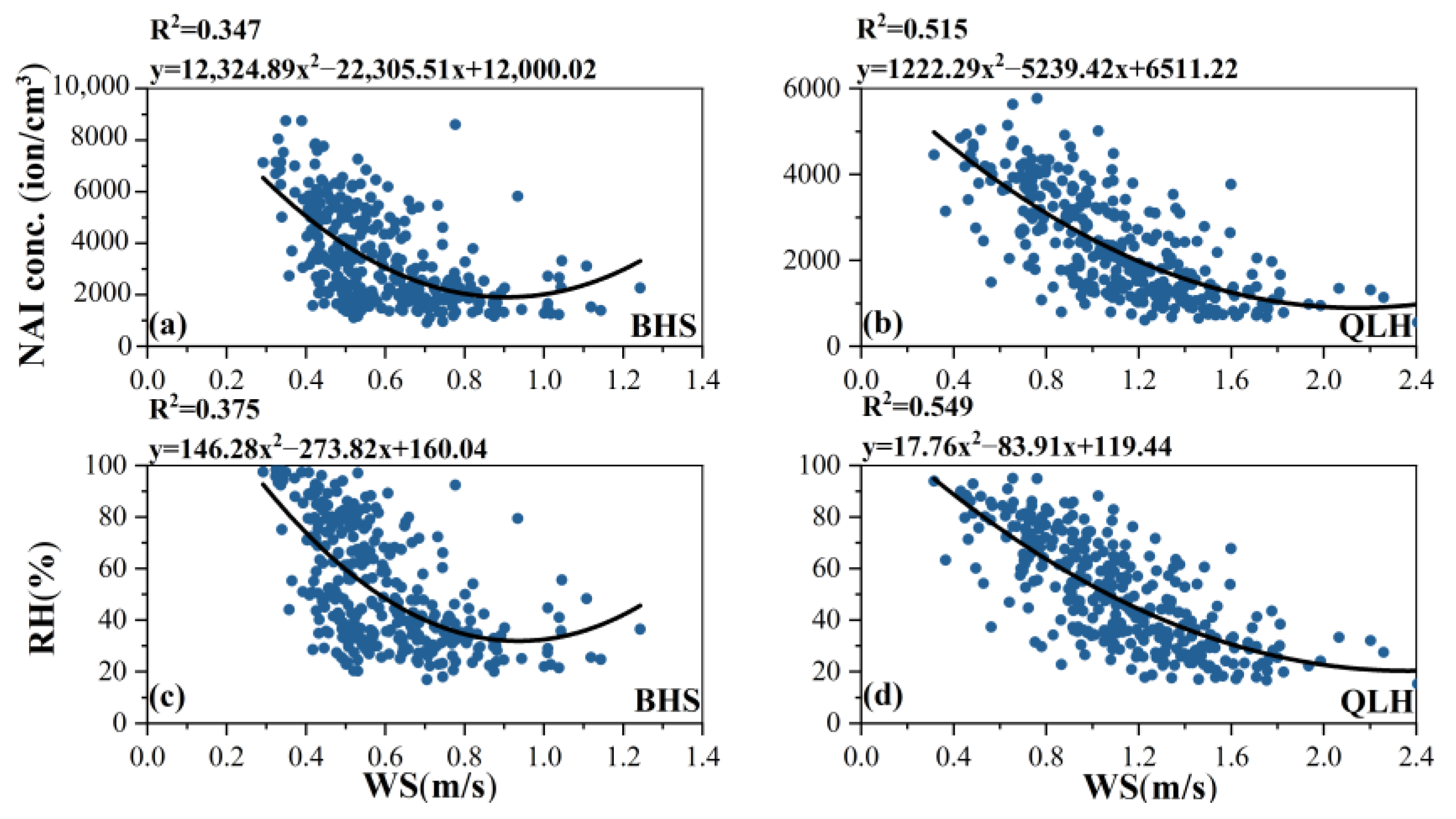
3.3.2. Correlation Analysis of the NAI Concentration and RH under Different WS Conditions

Figure 8 illustrates the correlation between NAI concentration and RH, incorporating WS as the third dimension. The results indicate that, within the low–value RH and NAI concentration interval, there is a concentration of scatter points in the high–value WS interval. This concentration indicates that high WS exerts an inverse influence on both RH and NAI concentration. In Figure 9, the correlation and R2 values between NAI concentration, RH, and WS are presented. The R2 values for NAI concentration and RH were 0.515 and 0.549, respectively, at the QLH site. These values were both higher than those observed at BHS (0.347 and 0.375). Figure 9 demonstrates that WS and NAI concentration display parallel trends with RH. It further reveals that at the BHS site, NAI concentration diminishes with increasing WS within the range of 0 to 0.94 m/s. Conversely, a reverse trend is observed when WS surpasses 0.94 m/s. Similarly, at the QLH site, the NAI concentration decreases with increasing WS between 0–2.14 m/s, but above this threshold, the relationship was found to be reversed.

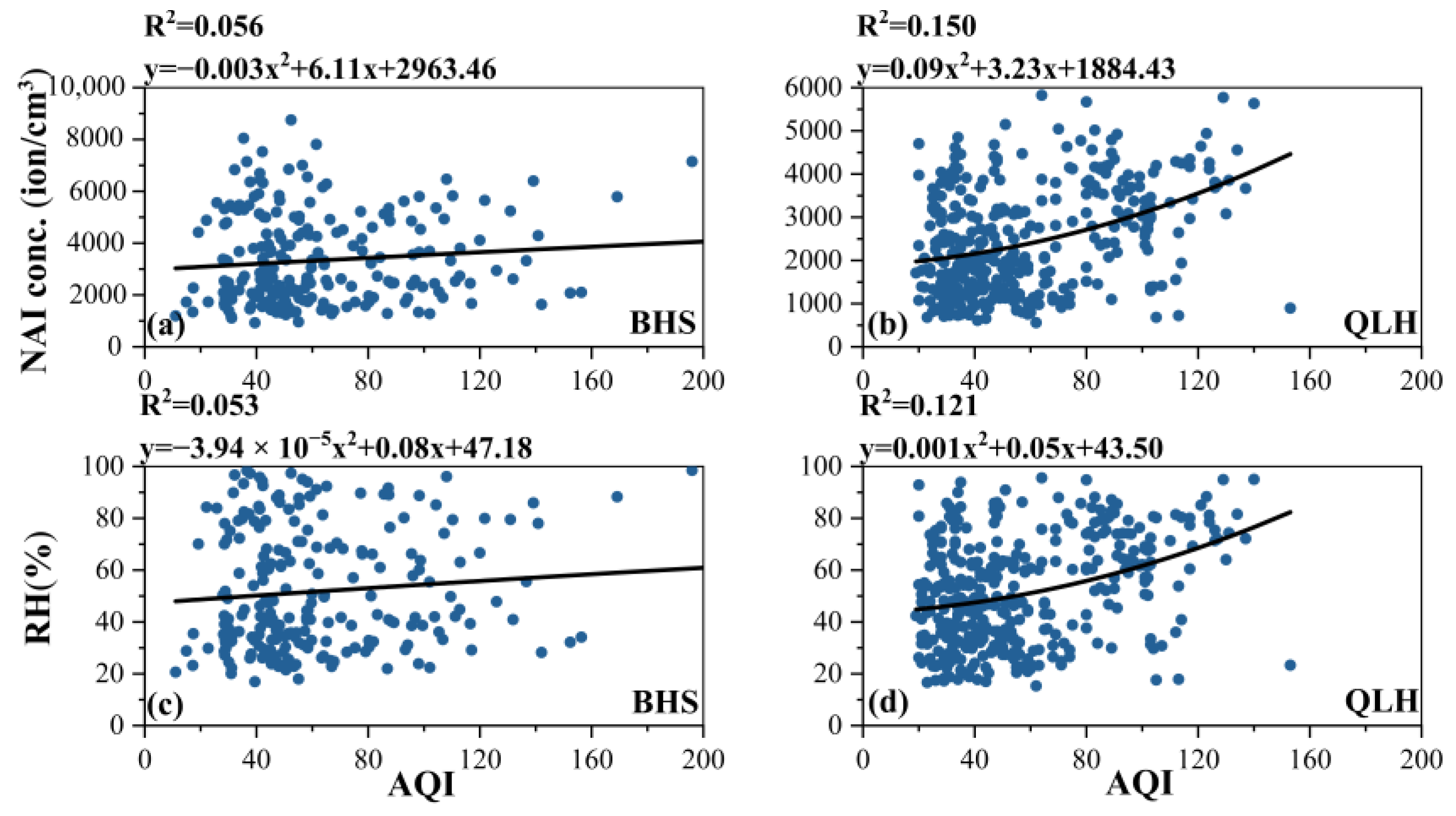
3.3.3. Correlation Analysis of the NAI Concentration and RH under Different AQI Levels

AQI was chosen for the correlation analysis owing to the influence of multiple pollutants on NAI concentration identified in the regression analysis. Given that the correlations among AQI, NAIs, and RH are identified as modestly weak (Figure A3 and Figure A4), we have accordingly placed the corresponding analytical diagrams in the appendices to facilitate a comprehensive presentation of the results. Readers seeking a detailed exploration of these intricate relationships are advised to consult the figures in the appendices. In Figure A4, the depiction of the relationship between NAI concentration, RH, and AQI is presented. Scatter points within different AQI intervals did not cluster in specific regions across these intervals. This lack of clustering indicates that AQI does not exert a substantial influence on either NAI concentration or RH. Figure A4 showcases the relationships among AQI, NAI concentration, and RH at both the BHS and QLH sites. For the BHS site, the R2 values are notably low, recorded at 0.056 and 0.053, respectively. Conversely, the QLH site exhibits slightly higher but still modest R2 values of 0.150 and 0.121. Collectively, these R2 values indicate a minimal impact of AQI on NAI concentration and RH.

3.3.4. Correlation Analysis of the NAI Concentration and RH under Different RN Levels

The analysis indicates that the correlations between RN, NAIs, and RH are relatively weak, similar to those found for AQI. Consequently, these results are included in the appendices (Figure A5 and Figure A6). In Figure A5, the scatter plots over different RN intervals show a lack of clustering, suggesting that RN has a minimal impact on NAIs and RH. Figure A6 reveals that that all R2 values are below 0.1, reinforcing the inference of RN’s minimal impact on NAI concentration and RH.

3.3.5. Structural Equation Analysis of Environmental Factors and NAI Concentration

In our research, we employed Structural Equation Modeling (SEM) to delve into the influence of various environmental factors on the concentration of NAIs and to ascertain any mediating variables. The models for both the BHS and QLH sites showed high similarity, reflecting the model’s generalizability. According to the SEM outcomes depicted in Figure 10, NAI concentration is predominantly governed by RH (BHS, ρRH,NAI = 0.92; QLH, ρRH,NAI = 0.94), with a mere measurement error of 0.07, indicating a substantial explanation of NAIs within the model. RH’s measurement error is more pronounced (BHS, 0.68; QLH, 0.65), implying that its influence extends beyond the model’s environmental variables to other factors like vegetation and rainfall. The environmental variables exert both direct and indirect impacts on NAI concentration. WS, TA, and AQI mainly influence NAIs indirectly via RH, whereas RN shows similar levels of indirect and direct impact. Specifically, WS predominantly impacts NAI concentration indirectly by negatively affecting RH (BHS, ρWS,RH = −0.47, ρWS,NAI = −0.01; QLH, ρWS,RH = −0.47, ρWS,NAI = −0.04), and TA positively influences NAI concentration indirectly through RH (BHS, ρTA,RH = 0.33, ρTA,NAI = 0.10; QLH, ρTA,RH = 0.22, ρTA,NAI = 0.13). RN’s overall impact on NAIs is relatively marginal, with comparable indirect and direct effects (BHS, ρRN,RH = −0.15, ρRN,NAI = −0.14; QLH, ρRN,RH = −0.17, ρRN,NAI = −0.17), and AQI’s overall effect on NAIs is even lesser, varying between the two sites (BHS, ρAQI,RH = −0.13, ρAQI,NAI = −0.03; QLH, ρAQI,RH = 0.16, ρAQI,NAI = −0.03). RN exhibits a marginal correlation with both WS and TA, each of which affect NAIs as well as mutually influencing one another.

4. Discussion

4.1. Investigating the Most Significant Environmental Factors That Influence NAI Concentration

This study investigated the correlation between NAI concentration and environmental factors. The results showed that RH exerted the most significant influence on NAI concentration across both natural forests and urban forests. Moreover, the linear regression of the NAI concentration against RH resulted in an R2 value of 0.93, providing robust evidence supporting RH’s pivotal role in driving changes in NAI concentration. These results are in line with previous research that identified RH as the primary environmental factor affecting NAI concentration in two urban parks in Shanghai, utilizing the random forest algorithm [23,24]. A study conducted in Wuyishan National Park similarly revealed weekly trends demonstrating a strong consistency between RH and NAI concentration. Subsequent multiple linear regression and correlation analyses confirmed a significant positive correlation [1]. The rise in RH influenced the predominant mechanisms involving particle collision and condensation. This effect amplified the condensation process, leading smaller particles to merge into larger ones. Consequently, this mitigated the loss of new aerosol formation, thereby preserving NAI concentration [40]. The research also highlighted a more pronounced shift in NAI concentration concerning RH during nighttime compared to daytime. This suggests a swifter alteration in NAI concentration and RH at night, attributed to the maintenance of high RH levels. Furthermore, reduced human activities contributed to decreased pollutant concentration, thereby slowing the dissipation of NAIs [37]. The R2 value at the QLH site was higher compared to that at the BHS site, indicating that RH in the urban forest had a marginally greater impact on NAI concentration than in the natural forest. This difference can be attributed to the distinct environmental characteristics of the two forest types. Natural forests typically feature taller canopies and greater depression, suggesting a more stable microclimate, which in turn leads to a more consistent relationship between NAI concentration and RH.

4.2. Diurnal, Seasonal, and Annual Dynamics of NAI Concentration and RH

Figure 3 illustrates the diurnal variation patterns of NAI concentration and RH in both urban forests and natural forests across all four seasons. Both types of forests exhibit relatively consistent diurnal variations, indicating that the differences in forest types do not affect the daily trends of NAI concentration. These variables exhibit their lowest values around midday and reach their peak during the nighttime. This finding is consistent with the results reported by Wang et al., who noted a U–shaped distribution of NAI concentration in the Wudalianchi, with a peak occurrence between 7:00–11:00 in the morning [22]. However, diverse diurnal variation patterns in NAI concentration have been reported across different regions. For instance, in mountain forests, Chen et al. [13] observed an increase in NAI concentration from 8:00 onwards, reaching its zenith in the afternoon (14:00–16:00). Li et al. [21] documented that in Wuyishan National Park, NAI concentration peaked during the early morning (0:00–6:00) and afternoon (14:00–15:00), while registering its lowest values during late morning (10:00–11:00) and early evening (18:00–19:00). Numerous factors influencing NAI concentration production include vegetation type [11,41], altitude [28], and canopy closure [13], potentially contributing to regional disparities. Figure A1 illustrates the synchronization between the increase in radiation and the decrease in NAI concentration and RH, as well as the reverse relationship. The increase in radiation led to a reduction in NAI concentration during the early morning, attributed to a decrease in the quantity of water molecules in the atmosphere, subsequently reducing the formation of ions by these molecules. The decline in NAI concentration at BHS occurred later than at QLH, possibly due to the inherent stability of natural forests compared to urban forests. The RH and the NAI concentration exhibited a decline with the onset of sunrise. While plant photosynthesis may have increased post–sunrise, leading to the production of more photosynthetic NAIs, the reduction in RH caused by sunrise had a more pronounced impact on NAIs, highlighting the significant role of RH in NAI concentration. After sunset, a decline in temperature attenuates atmospheric turbulent exchange, diminishing the mixing layer’s thickness and intensifying radiational cooling. These phenomena enhance atmospheric stability near the ground, thereby promoting the accumulation of relative humidity and NAI concentration at the forest’s surface. Concurrently, the reduction in human activities leads to lower air pollutant concentration, which is less prone to disperse from its sources, resulting in minimal pollutant levels within the forest. This scenario aids in diminishing the amalgamation of NAIs with pollutants and their subsequent deposition as dust. Collectively, these factors extend the lifespan of NAIs and elevate their concentration nocturnally.
On a daily basis, NAI concentration and RH consistently demonstrated a robust correlation, with RH exerting a predominant influence over changes in NAI concentration. Figure 5 displays a noteworthy increase in both NAI concentration and RH levels on rainy days, particularly during the non–rainy season. The months of June to August are characterized by consistently elevated levels of NAI concentration and RH, attributed to frequent rainfall. Rainfall augmented the quantity of water molecules in the air, aiding in the absorption of various pollutants. This, in turn, facilitated the combination of charged particles with water molecules, subsequently reducing the adsorption of pollutants and the deposition of dust associated with NAIs. The BHS site recorded a higher frequency of rainy days compared to QLH site, with notably more continuous rainfall during the summer months. Furthermore, observations indicate that the concentration levels at BHS were consistently higher than those at QLH, particularly in the summer season, thereby reinforcing the premise that rainfall positively impacts NAI concentration. Figure 4, illustrating seasonal average concentration, reveals that NAI concentration and RH peaked during the summer, experiencing a decline in autumn and winter, thereby supporting previous studies [19,21]. The variations were attributed to significant differences in rainfall, temperature, and vegetation growth status throughout the seasons [24]. Beijing’s continental monsoon climate, characterized by high humidity in summer and often accompanied by lightning, thunderstorms, and active plant photosynthesis, contributed significantly to the accumulation of NAIs. Comparing natural forests to urban green spaces, it was observed that NAI concentration was notably higher in natural forests. Interestingly, no significant difference in RH was noted, potentially due to the higher vegetation density in natural forests. The vegetation in natural forests exhibited more leaf tip activity, leading to the increased production of NAIs compared to urban forests. These findings offer valuable insights for citizens in choosing health–enhancing times for outdoor recreational activities.

4.3. How Do Other Environmental Factors Affect NAI Concentration and the Dominant Factor of NAI—RH?

4.3.1. How Does TA Affect NAI Concentration and RH?

This research explored the correlation between NAI concentration and RH under varying temperature conditions, as illustrated in Figure 6. A conspicuous stratification phenomenon emerged, revealing a distinct relationship between NAI concentration and RH across different temperature levels. Notably, high–temperature points were predominantly situated at elevated RH values, reinforcing the positive correlation established through both correlation and regression analyses. While this alignment was evident, no discernible clustering was observed among low–temperature points. Figure 7 illustrates that TA significantly impacts RH, WVD, and NAI concentration. The strongest correlation is observed between TA and WVD, with R2 values of 0.628 and 0.725, respectively. This is likely attributed to the rain–heat concurrent climate in Beijing, which manifests a pronounced daily correlation. Following in significance are the correlations of TA with RH and with NAI concentration, with the TA–RH correlation being slightly stronger than that of TA–NAI. This leads to the conclusion that TA predominantly affects RH by modifying WVD, subsequently increasing NAI concentration. However, TA can also directly influence NAI concentration through alternative mechanisms. For instance, elevated TA can enhance plant physiological processes, boosting NAI emission from leaf tips. Furthermore, TA may broadly affect atmospheric pressure, enhancing air circulation and particle collisions, resulting in reduced NAI concentration [23].

4.3.2. How Does WS Affect NAI Concentration and RH?

Previous research has unveiled a noteworthy direct correlation between WS and NAI concentration in the city parks of Shanghai [23]. It has been suggested that elevated WS levels facilitate the migration, dissipation, and collision of NAIs. Conversely, a study focusing on forest ecosystems revealed a contrasting relationship between WS and NAI concentration in linear regression models. Nevertheless, our study’s regression models indicated no significant correlation. The absence of correlation may be attributed to the intricate interplay between WS and NAIs. With increased WS, there is a potential for greater diffusion of pollutants and ground water vapor, leading to a reduction in NAI concentration in the surface atmosphere. Conversely, elevated air friction may lead to an increased production of NAIs. In Figure 8, a clustering of high–WS points within the high–NAI range, specifically in QLH, was observed. It is conceivable that high WS diminished surface water vapor density, contributing to a decrease in RH and NAI concentration. Compared to BHS, QLH exhibited lower canopy heights and smaller forest areas, rendering it less efficient at obstructing WS, thereby making WS at QLH a more substantial influence on NAI concentration and RH. Figure 9 illustrates that WS and NAI concentration exhibited similar trends with RH. This suggests that WS had a comparable impact on both NAI concentration and RH. Given that RH is the predominant environmental factor for NAI concentration, as discussed previously, we can infer that WS primarily influences NAI concentration by directly altering RH, thus indirectly affecting NAI concentration. WS demonstrated a negative correlation with NAI concentration, aligning with Pearson correlation results.

4.3.3. How Does AQI Affect NAI Concentration and RH?

Figure A3 reveals that clustering effects are negligible across different AQI intervals, demonstrating a minimal daily correlation between AQI, NAI concentration, and RH. Figure A4 highlights a markedly weak correlation in AQI, NAI concentration, and RH at the BHS site (NAI concentration, R2 = 0.056; RH, R2 = 0.053), in contrast to a slightly higher but still weak correlation at the QLH site (NAI concentration, R2 = 0.150; RH, R2 = 0.121). This disparity suggests a near non–existent relationship between NAI concentration and RH with AQI at the BHS site, whereas a modest correlation exists at the QLH site, potentially attributable to their distinct geographical settings. The remote, mountainous BHS site, distant from urban pollution sources, consistently exhibits low pollutant concentration and AQI, minimally impacting NAI concentration and RH. Conversely, the QLH site, situated nearer to urban centers, experiences more fluctuating pollutant concentration and AQI, significantly affecting NAI concentration and RH. Previous studies have identified air pollutants as significant factors affecting NAI concentration, such as Li et al. [21] confirming AQI as the key influencing factor in their study of urban green spaces in Fuyang District, Hangzhou, where high pollutant concentration due to dense human activity makes AQI an important factor affecting NAI concentration. The variability in study locations contributes to the differences in influencing factors on NAI concentration. Earlier research indicates that particulate matter tends to merge with NAIs, forming macromolecular precipitates and reducing NAI presence and stability [9]. Rising levels of O3 and NO2 promote atmospheric oxidation, facilitating the creation of secondary fine particles with complex structures and larger surface areas, which more effectively adsorb NAIs, consequently diminishing its concentration [42]. The impact of other AQI pollutants on NAI concentration, however, remains uncertain.

4.3.4. How Does RN Affect NAI Concentration and RH?

Figure A5 and Figure A6 do not indicate a discernible correlation between NAI concentration, RH, and RN. Previous research on the relationship between radiation and NAI concentration has predominantly focused on controlled indoor experiments [11,19], specifically emphasizing PAR and ultraviolet radiation (UV). For example, Wang et al. [19] explored the impact of PAR on the production of nitrogen–containing compounds derived from plants in both indoor and outdoor settings. The study’s findings revealed that NAI concentration increased with light intensity until reaching a plateau at saturation levels of PAR. Furthermore, the study demonstrated that PAR directly impacted plant growth and development, thereby influencing photosynthesis. Zhang et al. [17] conducted research on the impact of UVC on NAI concentration in an enclosed space, finding that NAI concentration increased with UVC exposure. However, in outdoor environments, the primary source of NAIs stemmed from UV–induced air ionization above 60 km in the atmosphere, with these particles gradually descending to the ground at a low rate [15]. UV only contributed to a small fraction of ground–level NAIs. Consequently, RN had the potential to influence NAI emissions. Nevertheless, it is essential to note that any related impact may be protracted and delayed. Thus, scatter plots in daily time intervals might not capture the nuanced influence of RN.

4.3.5. What Pathways Do Environmental Factors Use to Influence NAI Concentration?

Figure 10 presents a structural equation model depicting the influences of various environmental factors (WS, TA, RN, AQI, RH) on NAI concentration, exhibiting outstanding fit parameters that signify its precision and robustness. The models for both sites are remarkably similar, indicating consistent influence pathways between NAIs and meteorological factors across diverse forest types. NAI observation error is minimal, signifying a substantial contribution of the model to understanding NAI variation. Notably, RH and NAIs demonstrate high standardized regression coefficients, reiterating RH’s role as the principal factor influencing NAIs. Subsequently, TA and WS emerge as influential, with TA exerting both direct and more significant indirect positive effects on NAI concentration. The indirect effects predominantly arise from the unique climate of the Beijing region, characterized by concurrent rainy and hot seasons, whereas the direct effects stem from elevated TA enhancing plant physiological processes, thereby augmenting NAI emission from leaf tips. WS indirectly reduces NAI concentration by lowering RH in forested areas. The established relationships between these environmental factors and RH and NAIs in the SEM align with the deductions made in Section 4.3.1 and Section 4.3.2, thus offering scientific corroboration. Conversely, AQI and RN exert a less significant impact on NAIs and are not deemed major influencing factors. Notable correlations exist among environmental factors, particularly between TA and RN and WS and RN. Despite the intricate interplay of environmental factors on NAIs, RH consistently stands out as the principal determinant of NAI concentration.

5. Conclusions

This study explored the concentration of NAIs in both natural and urban forests, assessing the impact of various environmental factors. The research demonstrated a consistent relationship between RH and NAI concentration across multiple time scales in both types of forests, with the highest RH and NAI concentration observed during summer and nighttime on seasonal and daily scales, underscoring RH’s central role in NAI concentration changes. Further analysis established RH as the key factor affecting NAI concentration, with significant contributions from WS and TA. WS indirectly modifies NAI concentration via RH, whereas TA impacts NAI concentration both indirectly through RH and directly. Variations in forest types influence how factors such as AQI and WS impact NAI concentration due to differences in forest environmental stability. The climatic type and geographical features of the study area, specifically Beijing, influence NAI concentration dynamics, but this localization limits the study’s broader applicability to areas with different characteristics. The focus was on the effects of meteorological factors and pollutants in various forest types, excluding other influencing factors like vegetation characteristics, human activities, or altitude. Future research should expand to include a more diverse range of influencing factors and land covers. Many products [43,44,45] are known to accurately estimate the spatio–temporal distribution of influencing factors, and after the quantitative relationship between NAIs and influencing factors is established, estimating the spatial and temporal distribution of NAIs will be possible.

Author Contributions

Conceptualization, Y.Z., J.L. and Y.H.; methodology, Y.Z. and Y.H.; software, Y.H.; validation, J.L. and Y.H.; formal analysis, Y.H.; investigation, Y.H. and Y.L.; resources, J.L.; data curation, Y.H., H.G., F.X., Y.W. and S.H.; writing—original draft preparation, Y.H.; writing—review and editing, Y.Z., Y.H., J.L., H.G., F.X., Y.W. and S.H.; visualization, Y.Z. and Y.H.; supervision, J.L.; project administration, J.L. and Y.Z.; funding acquisition, J.L. All authors have read and agreed to the published version of the manuscript.

Funding

Research and Demonstration of Key Technologies for the Construction of the Capital Metropolitan National Park System (Z161100001116084).

Data Availability Statement

The data will be made available by the authors on request.

Conflicts of Interest

The authors declare no conflicts of interest.

Abbreviations

NAIsNegative air ions
TAAir temperature
RHRelative humidity
PAAir pressure
WDWind direction
WSWind speed
Pre.Precipitation
PARPhotosynthetically active radiation
RNNet radiation
UVUltraviolet radiation
UVAUltraviolet radiation A
UVCUltraviolet radiation C
SMCSoil moisture content
TSSoil temperature
AGFIAdjusted Goodness of Fit Index
RMSEARoot Mean Square Error of Approximation
CFIComparative Fit Index

Appendix A

Figure A1. Example diagram of equipment installation, using BHS site as an example. Radiation monitoring equipment is placed at a distance of 20 m, while monitoring equipment for air negative ion concentration, meteorological factors, and pollutants is placed at 2 m. Soil environment monitoring equipment is placed in the soil. Detailed information about the equipment can be found in Table 2.
Forests 15 00295 g0a1
Figure A2. Diurnal variations in hourly average of NAI concentration, RH, and RN across two distinct regions (BHS: (ad); QLH: (eh)) throughout different seasons (spring: (a,e); summer: (b,f); autumn: (c,g); winter: (d,h)).
Forests 15 00295 g0a2
Figure A3. Comparisons between NAI concentration and RH under different AQI conditions in two different regions (BHS: (a); QLH: (b)). Each dot represents the daily average concentration. AQI is represented as the third dimension and is indicated by different colors on the dots.
Forests 15 00295 g0a3
Figure A4. Correlations between of NAI concentration (a,b), RH (c,d), and AQI in two different regions (BHS: (a,c); QLH: (b,d)). Each dot represents the daily average concentration. The black lines represent the regression between NAI concentration, RH, and AQI. The R2 and the fitting formula are presented in the top left corner.
Forests 15 00295 g0a4
Figure A5. Comparisons between NAI concentration and RH under different RN conditions in two different regions (BHS: (a); QLH: (b)). Each dot represents the daily average concentration. RN is represented as the third dimension and is indicated by different colors on the dots.
Forests 15 00295 g0a5
Figure A6. Correlations between of NAI concentration (a,b), RH (c,d), and RN in two different regions (BHS: (a,c); QLH: (b,d)). Each dot represents the daily average concentration. The black lines represent the regression between NAI concentration, RH, and RN. The R2 and the fitting formula are presented in the top left corner.
Forests 15 00295 g0a6

References

  1. Li, C.; Xie, Z.; Chen, B.; Kuang, K.; Xu, D.; Liu, J.; He, Z. Different Time Scale Distribution of Negative Air Ions Concentrations in Mount Wuyi National Park. Int. J. Environ. Res. Public Health 2021, 18, 5037. [Google Scholar] [CrossRef]
  2. Goldstein, N. Reactive oxygen species as essential components of ambient air. Biochemistry 2002, 67, 161–170. [Google Scholar] [CrossRef] [PubMed]
  3. Lin, W.; Zeng, C.; Nie, W.; Nan, X.; Shen, S.; Shi, Y.; Yan, H.; Yang, F.; Wu, R.; Bao, Z. Study of the Vertical Structures, Thermal Comfort, Negative Air Ions, and Human Physiological Stress of Forest Walking Spaces in Summer. Forests 2022, 13, 335. [Google Scholar] [CrossRef]
  4. Liu, S.; Huang, Q.; Wu, Y.; Song, Y.; Dong, W.; Chu, M.; Yang, D.; Zhang, X.; Zhang, J.; Chen, C.; et al. Metabolic linkages between indoor negative air ions, particulate matter and cardiorespiratory function: A randomized, double-blind crossover study among children. Environ. Int. 2020, 138, 105663. [Google Scholar] [CrossRef] [PubMed]
  5. Wallner, P.; Kundi, M.; Panny, M.; Tappler, P.; Hutter, H.-P. Exposure to Air Ions in Indoor Environments: Experimental Study with Healthy Adults. Int. J. Environ. Res. Public Health 2015, 12, 14301–14311. [Google Scholar] [CrossRef]
  6. Yamada, R.; Yanoma, S.; Akaike, M.; Tsuburaya, A.; Sugimasa, Y.; Takemiya, S.; Motohashi, H.; Rino, Y.; Takanashi, Y.; Imada, T. Water-generated negative air ions activate NK cell and inhibit carcinogenesis in mice. Cancer Lett. 2006, 239, 190–197. [Google Scholar] [CrossRef]
  7. Goldstein, N.; Arshavskaya, T.V. Is atmospheric superoxide vitally necessary? Accelerated death of animals in a quasi-neutral electric atmosphere. Z. Naturforsch. C-A J. Biosci. 1997, 52, 396–404. [Google Scholar] [CrossRef]
  8. Huang, R.; Li, A.; Li, Z.; Chen, Z.; Zhou, B.; Wang, G. Adjunctive Therapeutic Effects of Forest Bathing Trips on Geriatric Hypertension: Results from an On-Site Experiment in the Cinnamomum camphora Forest Environment in Four Seasons. Forests 2023, 14, 75. [Google Scholar] [CrossRef]
  9. Ortiz-Grisales, P.; Patino-Murillo, J.; Duque-Grisales, E. Comparative Study of Computational Models for Reducing Air Pollution through the Generation of Negative Ions. Sustainability 2021, 13, 7197. [Google Scholar] [CrossRef]
  10. Bowers, B.; Flory, R.; Ametepe, J.; Staley, L.; Patrick, A.; Carrington, H. Controlled trial evaluation of exposure duration to negative air ions for the treatment of seasonal affective disorder. Psychiatry Res. 2018, 259, 7–14. [Google Scholar] [CrossRef]
  11. Zhang, Z.; Tao, S.; Zhou, B.; Zhang, X.; Zhao, Z. Plant stomatal conductance determined transpiration and photosynthesis both contribute to the enhanced negative air ion (NAI). Ecol. Indic. 2021, 130, 108114. [Google Scholar] [CrossRef]
  12. Wang, J.; Yang, Y.; Jiang, X.; Xiao, Y.; Deng, G.; Qian, Y.; Gu, X. Influence of meteorological conditions on the negative oxygen ion characteristics of well-known tourist resorts in China. Sci. Total Environ. 2022, 819, 152021. [Google Scholar] [CrossRef]
  13. Chen, Q.; Wang, R.; Zhang, X.; Liu, J.; Wang, D. Effects of Different Site Conditions on the Concentration of Negative Air Ions in Mountain Forest Based on an Orthogonal Experimental Study. Sustainability 2021, 13, 12012. [Google Scholar] [CrossRef]
  14. Tao, S.; Sun, Z.; Lin, X.; Zhang, Z.; Wu, C.; Zhang, Z.; Zhou, B.; Zhao, Z.; Cao, C.; Guan, X.; et al. Negative Air Ion (NAI) Dynamics over Zhejiang Province, China, Based on Multivariate Remote Sensing Products. Remote Sens. 2023, 15, 738. [Google Scholar] [CrossRef]
  15. Aubrecht, L.; Koller, J.; Stanek, Z. Onset voltages of atmospheric corona discharges on coniferous trees. J. Atmos. Sol.-Terr. Phys. 2001, 63, 1901–1906. [Google Scholar] [CrossRef]
  16. Harrison, R.G.; Carslaw, K.S. Ion-aerosol-cloud processes in the lower atmosphere. Rev. Geophys. 2003, 41. [Google Scholar] [CrossRef]
  17. Zhang, J.; Yu, Z. Experimental and simulative analysis of relationship between ultraviolet irradiations and concentration of negative air ions in small chambers. J. Aerosol Sci. 2006, 37, 1347–1355. [Google Scholar] [CrossRef]
  18. Wu, C.; Chu, T.; Chen, S.; Wu, S. Generating Negative Air Ions in Construction Waterscapes at a Garden Scale. Environments 2019, 6, 100. [Google Scholar] [CrossRef]
  19. Wang, J.; Li, S.-h. Changes in negative air ions concentration under different light intensities and development of a model to relate light intensity to directional change. J. Environ. Manag. 2009, 90, 2746–2754. [Google Scholar] [CrossRef]
  20. Tikhonov, V.P.; Tsvetkov, V.D.; Litvinova, E.G.; Sirota, T.V.; Kondrashova, M.N. Generation of negative air ions by plants upon pulsed electrical stimulation applied to soil. Russ. J. Plant Physiol. 2004, 51, 414–419. [Google Scholar] [CrossRef]
  21. Li, A.; Li, Q.; Zhou, B.; Ge, X.; Cao, Y. Temporal dynamics of negative air ion concentration and its relationship with environmental factors: Results from long-term on-site monitoring. Sci. Total Environ. 2022, 832, 155057. [Google Scholar] [CrossRef] [PubMed]
  22. Wang, H.; Wang, B.; Niu, X.; Song, Q.; Li, M.; Luo, Y.; Liang, L.; Du, P.; Peng, W. Study on the change of negative air ion concentration and its influencing factors at different spatio-temporal scales. Glob. Ecol. Conserv. 2020, 23, e01008. [Google Scholar] [CrossRef]
  23. Luo, L.; Sun, W.; Han, Y.; Zhang, W.; Liu, C.; Yin, S. Importance Evaluation Based on Random Forest Algorithms: Insights into the Relationship between Negative Air Ions Variability and Environmental Factors in Urban Green Spaces. Atmosphere 2020, 11, 706. [Google Scholar] [CrossRef]
  24. Miao, S.; Zhang, X.; Han, Y.; Sun, W.; Liu, C.; Yin, S. Random Forest Algorithm for the Relationship between Negative Air Ions and Environmental Factors in an Urban Park. Atmosphere 2018, 9, 463. [Google Scholar] [CrossRef]
  25. Shi, G.; Zhou, Y.; Sang, Y.; Huang, H.; Zhang, J.; Meng, P.; Cai, L. Modeling the response of negative air ions to environmental factors using multiple linear regression and random forest. Ecol. Inform. 2021, 66, 101464. [Google Scholar] [CrossRef]
  26. Yoon, Y.; Lee, S.H.; Kim, J.H. Evaluation of Air Ion According to Vegetation Types in Valleys and Slopes-Focused on Tangeumdae Park in ChungJu. J. Environ. Sci. Int. 2020, 29, 519–529. [Google Scholar] [CrossRef]
  27. Yan, X.; Wang, H.; Hou, Z.; Wang, S.; Zhang, D.; Xu, Q.; Tokola, T. Spatial analysis of the ecological effects of negative air ions in urban vegetated areas: A case study in Maiji, China. Urban For. Urban Green. 2015, 14, 636–645. [Google Scholar] [CrossRef]
  28. Wang, R.; Chen, Q.; Wang, D. Effects of Altitude, Plant Communities, and Canopies on the Thermal Comfort, Negative Air Ions, and Airborne Particles of Mountain Forests in Summer. Sustainability 2022, 14, 3882. [Google Scholar] [CrossRef]
  29. Wang, W.; Xia, S.; Zhu, Z.; Wang, T.; Cheng, X. Spatiotemporal distribution of negative air ion and PM2.5 in urban residential areas. Indoor Built Environ. 2022, 31, 1127–1141. [Google Scholar] [CrossRef]
  30. Shi, G.; Huang, H.; Sang, Y.; Cai, L.; Zhang, J.; Cheng, X.; Meng, P.; Sun, S.; Li, J.; Qiao, Y. Solar-induced chlorophyll fluorescence intensity has a significant correlation with negative air ion release in forest canopy. Atmos. Environ. 2022, 269, 118873. [Google Scholar] [CrossRef]
  31. Cui, H.; Li, Z.; Cao, R. Relationships between the Negative Air Ions and Meteorological Factors in Different Forest Villages of Taiyue Moutain. J. West China For. 2022, 51, 27–34. (In Chinese) [Google Scholar] [CrossRef]
  32. Fang, Y.; Zhang, F.; Chen, L.; Li, B.; Wang, H. Correlation analysis of negative air ion concentration and meteorological factors in Jiangxi. J. Meteorol. Sci. 2022, 42, 254–260. (In Chinese) [Google Scholar]
  33. Cai, L.; Wang, C.; Zhang, J.; Meng, P.; Shi, G. The influence mechanism of negative air ion in forest ecosystem based on structural equation. Acta Ecol. Sin. 2024, 44, 1–9. (In Chinese) [Google Scholar] [CrossRef]
  34. Shi, G.; Zhou, Y.; Sang, Y.; Zhang, J.; Meng, P.; Cai, L.; Pei, S.; Wang, Y. Influence of Environmental Factors on Negative Air Ion Using Random Forest Algorithm. Chin. J. Agrometeorol. 2021, 42, 390–401. (In Chinese) [Google Scholar] [CrossRef]
  35. Wang, W.; Zhang, Z. Spatio-temporal Change of Negative Air Ion Concentration of Urban Residential Area and Air Quality Assessment—Case Study of Hefei City. Ecol. Environ. Sci. 2014, 23, 1783–1791. (In Chinese) [Google Scholar] [CrossRef]
  36. Yu, H.; Xin, X.; Pei, S.; Wu, D.; Wu, S.; Fa, L.; Ma, S.; Guo, H. Characteristics of air anion change and its relationship with meteorological factors in forest margin area of Jiulong Mountain. Ecol. Sci. 2018, 37, 191–198. (In Chinese) [Google Scholar] [CrossRef]
  37. Zhu, S.; He, Q.; Su, Y.; Cui, G.; Li, J. Negative air ion concentration and its influencing factors of urban forest in different geographical spaces. J. Beijing For. Univ. 2023, 45, 66–77. (In Chinese) [Google Scholar]
  38. Li, J.; Gao, T.; Chen, K.; Lu, J.; Zheng, W.; Fan, Z. Characteristics of Negative Air Ion Concentration and Its Relationships with Meteorological Factors in Abies georgei var.smithii Forest of Southeast Tibet. J. Northeast. For. Univ. 2021, 49, 77–82. (In Chinese) [Google Scholar] [CrossRef]
  39. Shi, G.; Sang, Y.; Zhang, J.; Meng, P.; Cai, L.; Pei, S. Relationship between Negative Air Ion and Relative Humidity in Quercus variabilis Plantation under Natural Conditions. Chin. J. Agrometeorol. 2021, 42, 24–33. (In Chinese) [Google Scholar]
  40. Skalny, J.D.; Mikoviny, T.; Matejcik, S.; Mason, N.J. An analysis of mass spectrometric study of negative ions extracted from negative corona discharge in air. Int. J. Mass Spectrom. 2004, 233, 317–324. [Google Scholar] [CrossRef]
  41. Ling, D. Review on research of the negative air ion concentration distribution and its correlation with meteorological elements in mountain tourist area. Earth Sci. 2019, 8, 60–68. [Google Scholar] [CrossRef]
  42. Zhao, Q.; Li, L.; Li, H. Research progress on surface ozone pollution in domestic and overseas. Environ. Sci. Technol. 2018, 31, 72–76. (In Chinese) [Google Scholar]
  43. Wei, J.; Li, Z.; Wang, J.; Li, C.; Gupta, P.; Cribb, M. Ground-level gaseous pollutants (NO2, SO2, and CO) in China: Daily seamless mapping and spatiotemporal variations. Atmos. Chem. Phys. 2023, 23, 1511–1532. [Google Scholar] [CrossRef]
  44. Shi, H.; Yang, D.; Wang, W.; Fu, D.; Gao, L.; Zhang, J.; Hu, B.; Shan, Y.; Zhang, Y.; Bian, Y.; et al. First estimation of high-resolution solar photovoltaic resource maps over China with Fengyun-4A satellite and machine learning. Renew. Sustain. Energy Rev. 2023, 184, 113549. [Google Scholar] [CrossRef]
  45. Gelaro, R.; McCarty, W.; Suarez, M.J.; Todling, R.; Molod, A.; Takacs, L.; Randles, C.A.; Darmenov, A.; Bosilovich, M.G.; Reichle, R.; et al. The Modern-Era Retrospective Analysis for Research and Applications, Version 2 (MERRA-2). J. Clim. 2017, 30, 5419–5454. [Google Scholar] [CrossRef]
Figure 1. Map and instrument installation location of the research area.
Forests 15 00295 g001
Figure 2. The correlation between observations of RH and NAI concentration metrics in two distinct regions (BHS: (a); QLH: (b)) during daytime and nighttime. The red dots represent nightly average values, while the blue dots represent daily average values. The blue and red lines, respectively, depict the regression between RH and NAI concentration during daytime and nighttime. The coefficient of determination R2 and the fitting formula corresponding to the colors are displayed in the top left corner of the figures.
Forests 15 00295 g002
Figure 3. Diurnal variations in hourly average of NAI concentration and RH across two distinct regions (BHS: (ad); QLH: (eh)) throughout different seasons (spring: (a,e); summer: (b,f); autumn: (c,g); winter: (d,h)). The blue line represents the trend in NAI concentration, while the red line depicts the trend in RH.
Forests 15 00295 g003
Figure 4. The average values of NAI concentration and RH in two distinct regions across different seasons. NAI concentration and RH are visually differentiated by color, with the blue color representing NAI concentration and the red color representing RH. The regions are distinguished by distinct patterns, where left diagonal lines denote BHS, and crossed diagonal lines signify QLH.
Forests 15 00295 g004
Figure 5. The annual trends of NAI concentration and RH in two different regions (BHS: (a); QLH: (b)). The blue line denotes the variation trend of daily average NAI concentration, while the red line illustrates the variation trend of daily average RH. Additionally, the shaded area in the graph represents days with recorded precipitation.
Forests 15 00295 g005
Figure 6. Comparisons between NAI concentration and RH under different TA conditions in two distinct regions (BHS: (a); QLH: (b)). Each dot in the scatter plot represents the daily average concentration, with TA depicted as the third dimension through different colors on the dots.
Forests 15 00295 g006
Figure 7. The correlation between NAI concentration (a,b), RH (c,d), WVD (e,f), and TA in two different regions (BHS: (a,c,e); QLH: (b,d,f)). Each dot represents the daily average concentration, and the black lines represent the regression between NAI concentration, RH, WVD, and TA. The R2 values and the fitting formula are presented in the top left corner.
Forests 15 00295 g007
Figure 8. Comparisons between NAI concentration and RH combined under different WS conditions at BHS (a) and QLH (b). Each dot represents the daily average concentration. WS is represented as the third dimension and is indicated by different colors on the dots.
Forests 15 00295 g008
Figure 9. Correlations between NAI concentration (a,b), RH (c,d), and WS in two different regions (BHS: (a,c); QLH: (b,d)). Each dot represents the daily average concentration. The black lines represent the regression between NAI concentration, RH, and WS. The R2 and the fitting formula are presented in the top left corner.
Forests 15 00295 g009
Figure 10. Structural equation model of environmental factors and negative air ions. Solid lines with arrows in the diagrams are labeled with standardized regression coefficients (ρ ranging from −1 to 1), with the width of each line representing the parameter’s magnitude. (a) Illustrates the BHS site, while (b) depicts the QLH site. Dashed lines indicate correlation relationships, whereas circles denote measurement errors. In these figures, blue and red lines signify significant negative and positive impacts, respectively (p < 0.05).
Forests 15 00295 g010
Table 1. Summary of key influencing factors on NAI concentration.
SiteClimate TypeSite TypePeriodDominant Factors
South Korea, ChungJu, Tangeumdae Park [26]Warm temperate monsoon climateUrban forestsAugust 2018Diameter at
breast height
China, Gansu Province, the suburb of Tianshui [27]Continental semi–humid monsoon climateCroplands2–6 August to 11–15 October 2013Air temperature, SO2, NOx, aerosols, altitude
Artificial forests
Greenbelts
Natural forests
China, Shaanxi Province, the Taibai Mountain National Forest Park [28]Continental semi–humid monsoon climateNatural forestsJuly–August 2021Altitude, plant communities, canopy characteristics, canopy density, canopy porosity, leaf area index, sky view factor
China, Sichuan Province, Zoige Wetland Nature Reserve [12]Humid monsoon climate of the highland coldGreenbeltsJune 2020
January 2020
Atmospheric supersaturation, condensation rate, atmospheric aerosol, retention index, cloud parameters
China, Zhejiang Province, Hangzhou West Lake [12]Humid subtropical monsoon climateWater bodies
Hangzhou urban areas [12]Urban built–up areas
China, Heilongjiang Province, Wudalianchi Scenic Area [22]Northeast temperate continental monsoon climateOpen spacesAugust–September 2018Ozone, humidity, types of landscape
Water bodies
Forests
China, Zhejiang Province [14]Humid subtropical monsoon climateForests, water bodies, barrens, grasslands, croplands, urban built–up areas2018–2020Solar–induced chlorophyll fluorescence
China, Henan Province, Yellow River Xiaolangdi Site [25]Warm temperate monsoon climateMixed forests1 May–1 October 2019 and 2020PM2.5, soil moisture, relative humidity
China, Shanghai City, Zhongshan Park [24]Subtropical monsoon climateUrban forestsMarch 2017–February 2018Relative humidity
China, Zhejiang Province, Hangzhou Fuyang District [21]Humid subtropical monsoon climate prevailsUrban forestsJuly 2019–March 2021Air quality index
China, Shaanxi Province, Taibai Mountain National Forest Park [13]The transition zone between subtropical and warm temperate climates.Natural forests1–5 May 2021Altitude, canopy density
China, Anhui Province, city centre of Hefei [29]Subtropical humid monsoon climateUrban built–up areas2019Temperature, relative humidity
China, Henan Province, Xiaolangdi Site [30]Warm temperate continental monsoon climateNatural forests1 June–1 October 2019Solar–induced chlorophyll fluorescence intensity
China, Henan Province, Minquan County [30]Barren1 August–1 October 2020
China, Fujian Province, the Mount Wuyi National Park [1]Central subtropical humid monsoon climateNatural forestsOctober 2018–20 February 2020Relative humidity, precipitation
China, Shanxi Province, Taiyue Mountain Site [31]Warm temperate continental monsoon climateWater bodies and forestsJuly 2021Air temperature, relative humidity
Low mountain forestsAir temperature and precipitation
Low mountain meadowLight and effective radiation, soil moisture
China, Jiangxi Province, Jing’an observation base [32]Humid north subtropical climateArtificial forests1 January–31 December 2019PM2.5, saturated vapor pressure difference, wind speed
China, Henan Province, Xiaolangdi critical zone [33,34]Warm temperate continental monsoon climateArtificial forestsJune–September 2020Wind speed, air temperature, relative humidity
June–September 2018 and 2019Air humidity
China, Anhui Province, Hefei City [35]Subtropical humid monsoon climateUrban built–up areasAugust 2013–January 2014Relative humidity, air temperature
China, Beijing, Jiulong Mountain [36]Warm temperate east coast continental monsoon climateArtificial forestsSeptember 2017 and October 2017Suburban: oxygen, wind speed, air temperature
China, Guangdong Province, Shimen National Forest Par [37]South subtropical monsoon climateSuburban urban artificial forestsSeptember 2019–January 2020
May–August 2020
Air temperature
China, Guangdong Province, Longyandong Forest Farm Maofeng Work Area [37]Near suburban artificial forestsAir temperature
China, Guangdong Province, Changgangshan Nature Reserve [37]Downtown urban artificial forestsAir temperature, ultraviolet radiation
China, Guangdong Province, Wushan Street [37]Urban built–up areasAir temperature, relative humidity
China, Tibet Province, Sejila Mountain National Forest Park [38]Humid north subtropical climateNatural forests1 September 2017–30 November 2019Air temperature, precipitation
Table 2. Environmental monitoring parameters and sensor specifications summary.
ClassificationFactorsData SensorsUnitMeasuring Accuracy
NAIsFYLZ–200 monitorions/cm3≤±15%
Meteorological factorsTAHMP155A model°C≤±0.17 °C
RH%≤±1.7%
PA (air pressure)ATMOS modelkpa±0.05 kPa
WD (wind direction)034B°±4°
WSm/s±0.11 m/s (<10.1 m/s)
±1.1% (>10.1 m/s)
Prec. (precipitation)TE525mm±1% (≤10 mm/h)
+0, −3% (10~20 mm/h)
+0, −5% (20~30 mm/h)
Radiation factorsPAR (photosynthetically
active radiation)
LI–190Rµmol/m2/s5 μA~10 Μa/1000 μmol s*m2
RN (net radiation)CNR4W/m2<4% (−10 °C~+40 °C)
UVA
(ultraviolet radiation A)
SU–200W/m2<10%
Soil factorsSMC (soil moisture content)TEROS11m3/m3±0.01~0.02 m3/m3
TS (soil temperature)°C±1 °C (−40~0 °C)
±0.5 °C (0~60 °C)
Air quality factorsO3O342eμg/m3±1%
COCO12emg/m3±1%
SO2AF22eμg/m3±1%
NOAC32eμg/m3±1%
NO2μg/m3±1%
NOXμg/m3±1%
PM2.5MP101Mμg/m30.5 µg/m3
PM10μg/m30.5 µg/m3
Table 3. The Pearson correlation coefficient.
ClassificationFactorsBHS’s
Correlation Coefficient
QLH’s
Correlation Coefficient
Meteorological factorsRH0.967 **0.978 **
TA0.392 **0.429 **
PA−0.294 **−0.432 **
Prec.0.408 **0.317 **
WD0.057−0.250 **
WS−0.525 **−0.689 **
Radiation factorsPAR−0.104−0.142 **
RN0.158 **0.144 **
UVA−0.117 *−0.156 **
Soil factorsSWC0.413 **0.211 **
TS0.444 **0.422 **
Air quality factorsSO20.064−0.194 **
NOX0.075−0.012 **
CO0.143 *−0.067
O30.1010.355 **
PM100.0580.093
PM2.50.130 *0.384 **
NO−0.228 **0.020
NO2−0.139 **0.025
Note: * p < 0.05, ** p < 0.01. Correlation coefficient indicates the Pearson correlation coefficient between environmental factors and NAI concentration.
Table 4. Multivariate linear best regression model.
Unstandardized FactorStandardized Factor
ModelBSEΒetatSigR2
BHSConstant−146.69268.658 −2.1370.034
RH68.4851.0570.89764.7980.000
Prec.51,842.4716994.4300.0957.4120.000
TS18.2753.0840.0935.9250.0000.968
NO−50.99616.439−0.039−3.1020.002
RN−1.6250.434−0.055−3.7470.000
NO2−8.7574.331−0.025−2.0220.044
QLHConstant−257.42748.125 −5.3490.000
RH54.3580.6760.93080.4550.000
TA34.7475.6720.3166.1260.000
RN−2.0820.334−0.113−6.2370.000
NOX−4.3760.877−0.063−4.9900.0000.973
Prec.322,590.439101,107.5650.0333.1910.002
TS−17.3435.564−0.159−3.1170.002
SO2−10.6403.673−0.029−2.8970.004
Disclaimer/Publisher’s Note: The statements, opinions and data contained in all publications are solely those of the individual author(s) and contributor(s) and not of MDPI and/or the editor(s). MDPI and/or the editor(s) disclaim responsibility for any injury to people or property resulting from any ideas, methods, instructions or products referred to in the content.

