Regional Forest Structure Evaluation Model Based on Remote Sensing and Field Survey Data

Abstract

The assessment of a forest’s structure is pivotal in guiding effective forest management, conservation efforts, and ensuring sustainable development. However, traditional evaluation methods often focus on isolated forest parameters and incur substantial data acquisition costs. To address these limitations, this study introduces a cost-effective and innovative evaluation model that incorporates remote sensing imagery and machine learning algorithms. This model holistically considers the forest composition, the tree age structure, and spatial configuration. Using a comprehensive approach, the forest structure in Longquan City was evaluated at the stand level and categorized into three distinct categories: good, moderate, and poor. The construction of this evaluation model drew upon multiple data sources, namely Sentinel-2 imagery, digital elevation models (DEMs), and forest resource planning and design survey data. The model employed the Recursive Feature Elimination with Cross-Validation (RFECV) method for feature selection, alongside various machine learning algorithms. The key findings from this research are summarized as follows: The application of the RFECV method proved effective in eliminating irrelevant factors, reducing data dimensionality and, subsequently, enhancing the model’s generalizability; among the tested machine learning algorithms, the CatBoost model emerged as the most accurate and stable across all the datasets; specifically, the CatBoost model achieved an impressive overall accuracy of 88.07%, a kappa coefficient of 0.6833, and a recall rate of 76.86%. These results significantly surpass the classification precision of previous methods. The forest structure assessment of Longquan City revealed notable variations in the forest quality distribution. Notably, forests classified as “good” quality comprised 11.18% of the total, while “medium” quality forests constituted the majority at 76.77%. In contrast, “poor” quality forests accounted for a relatively minor proportion of the total, at 12.05%. The distribution findings provide valuable insights for targeted forest management and conservation strategies.

1. Introduction

Forests fulfill critical ecological functions, such as water nourishment, climate regulation, air purification, carbon sequestration, oxygen release, nutrient accumulation, and biodiversity preservation [1]. The forest structure is the configuration and distribution of trees, including the species composition, spatial arrangement, and tree age distribution within a forest ecosystem. Understanding this structure is essential for grasping the evolutionary history and current state of ecosystems, thereby guiding sustainable forest management practices [2,3]. Forest structure evaluation involves qualitative and quantitative analyses of the ecosystem’s composition, requiring a thorough examination of various forest attributes. This comprehensive assessment necessitates significant data to meet the requirements of the evaluation. While traditional field surveys are reliable for forest resource monitoring and management, they can be time consuming, laborious, and expensive [4]. Therefore, integrating diverse data sources to leverage the synergistic effects is crucial for accurately evaluating forest structures.

The traditional methods of assessing a forest’s ecological quality involve thoroughly examining the diverse aspects of the forest ecosystem. These methods require extensive field survey data to facilitate a comprehensive and detailed understanding of the current state of forest resources and the systematic monitoring of the forest’s ecological quality [5]. However, they are also expensive, time consuming, and labor intensive. For instance, the forest resource planning and design survey is a very important type of forest investigation, with massive sub-compartments (the basic unit of inventory for forest management planning and design, divided by the terrain boundaries, including the ridge line, valleys, roads, etc., or forest ownership boundaries, with a maximum area of 15 ha in south China and 25 ha in other parts of China) as the basic inventory unit [6,7,8]. In China, the number of forest sub-compartments in almost every province is over one million.

In recent years, remote sensing technology has seen rapid advancements, facilitating the dynamic, efficient, and comprehensive monitoring of forest resources. The eight spectral bands of the WorldView-2 satellite are employed to classify ten tree species, with the importance of each band being ranked [9]. Landsat 8 provides accurate data for monitoring forest canopy closure, supplying crucial information for resource management [10]. Sentinel-1 radar remote sensing effectively estimates aboveground biomass, enhancing forest structure analysis [11]. Airborne C-band polarimetric interferometry differentiates forests of varying tree age classes, furthering forest classification research [12]. The forest height in state-owned forests in Hunan Province is determined using L-band ALOS-2 PALSAR-2 radar data, thereby improving measurement accuracy [13]. While studies examining forest structure-related parameters using optical or radar remote sensing data alone have yielded encouraging outcomes, reliance on a single remote sensing source inherently presents specific constraints, preventing the acquisition of exhaustive forest resource information [14].

Recently, an increasing number of researchers have exploited the synergy of diverse datasets to estimate parameters related to forest structure, leading to notable advancements. Combining Geoeye-1 multispectral imagery with LiDAR data enhances the accuracy of urban forest tree species classification [15]. Integrating multi-temporal radar satellite data with Sentinel-1 information facilitates a more accurate estimation of tree heights in mountainous forests [16]. The combination of the Landsat satellite temporal series with LiDAR data improves forest canopy coverage and stature estimation [17]. Standalone unmanned aerial vehicle laser scanning and terrestrial laser scanning data have been proven to accurately estimate forest tree metrics [18]. Numerous studies demonstrate that amalgamating multi-source remote sensing data can provide more comprehensive forest resource information and effectively enhance the accuracy of estimating forest structure-related parameters. Nevertheless, there remains considerable untapped potential in applying this approach to the assessment of forest structures.

Machine learning methods are powerful tools for data-driven analysis involving forest ecosystems [19]. The Random Forest algorithm was effectively utilized to estimate forest ecological function levels, yielding commendable results [20]. Furthermore, integrating the gradient boosting model, with differential evolution, facilitates regional analysis of soil organic carbon reserves in arid forests, thereby highlighting the potential of machine learning in addressing data scarcity issues [21]. Initially, during model development, the features are often directly extracted from the raw data. However, as the number of features increases, so does the volume of data processed by the model, potentially causing computational delays and efficiency setbacks. An excessive number of features may cause data redundancy and noise [22]. Therefore, it becomes imperative to employ feature selection techniques and reduce data dimensionality strategically to optimize model performance and minimize the training duration [23]. Combining feature selection methods and machine learning algorithms can significantly improve model performance in mapping mangrove forests [24]. These studies underscore the remarkable potential of machine learning methods in regard to forest ecosystems and structural research, offering economical, efficient, and accurate data analysis solutions.

Based on multi-source data, this paper employs four machine learning algorithms to evaluate forest structure. A comprehensive evaluation of the forest structure in Longquan City is undertaken, considering key aspects, such as forest composition, age–class structure, and spatial configuration. The forests are, subsequently, categorized into three categories: good, medium, and poor. The data sources include Sentinel-2 imagery, digital elevation models (DEMs), and the data related to the forest resource planning and design survey. A comparative analysis is conducted for four machine learning algorithms: K-Nearest Neighbor (KNN), Support Vector Machine (SVM), Random Forest (RF), and CatBoost. Following a thorough comparative analysis of their performance, the most suitable algorithm is chosen for modeling and evaluating forest structural grades.

2. Materials and Methods

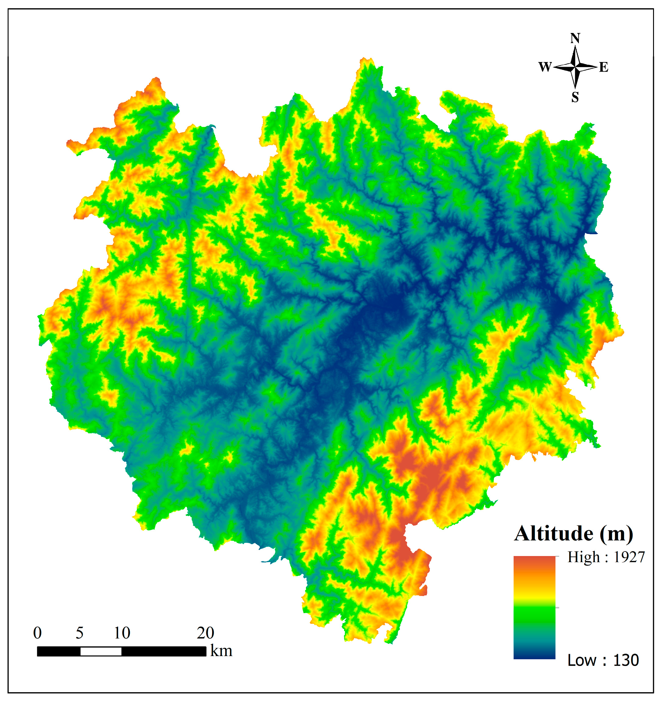
2.1. Overview of the Study Area

Longquan City, located in the southwest of Zhejiang Province, is positioned between 27°42′ and 28°20′ N latitude, as well as 118°42′ and 119°25′ E longitude. Spanning a distance of 70.25 km from east to west and 70.80 km from north to south, it covers a vast area of 3059 km². Longquan City lies within the subtropical monsoon climate zone, boasting an impressive forest coverage rate of 84.2%, rich biodiversity, and abundant natural resources. The average annual temperature is 17.6 °C, coupled with an annual precipitation of 1699.4 mm, and an annual relative humidity averaging 79%. The administrative distribution map of Longquan City is illustrated in Figure 1. All remote sensing figures in this study are drawn from using ArcMap 10.8 (ESRI 2011; ArcGIS Desktop: Release 10.8, Redlands, CA, USA; Environmental Systems Research Institute).

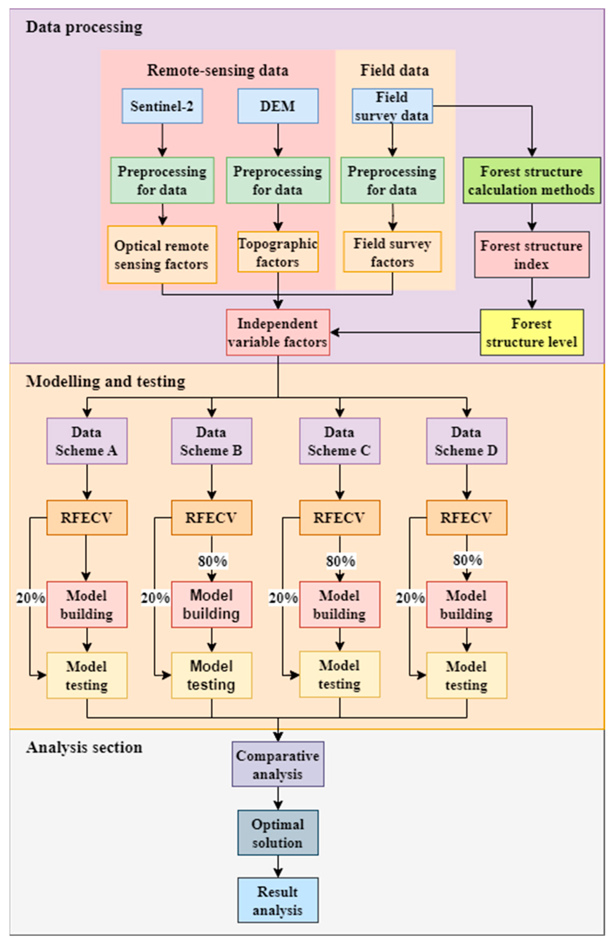
2.2. Research Framework

The research framework (as shown in Figure 2) included three components: data processing, modelling and testing, and the analysis section. During the data processing, Sentinel-2 remote sensing data, DEMs, and field survey data were preprocessed to extract the key characteristic factors. This study adopts the sub-compartment as the basic evaluation unit. By referencing the corresponding formulas in the “Monitoring Indicator System and Technological Specification of Forest Ecological Quality” (T/CSF 002-2021), using field survey data, the forest structure index (FSI) for each sub-compartment was calculated [25]. Subsequently, these indices served as the basis for evaluating the forest structure levels of the sub-compartments [6]. During the modelling and testing, four distinct data combination schemes were adopted. Subsequently, the RFECV method was used for each data scheme to screen the feature factors. Afterwards, 80% of the data were allocated to the training set, while the remaining 20% were designated as the test set. By comparing the results using the test set, the best data scheme and the optimal machine learning model were identified. Finally, a comprehensive analysis of the results based on a combination of the best data scheme and optimal machine learning model was conducted.

2.3. Data Sources and Preprocessing

2.3.1. Data Sources

This study adopted a comprehensive set of data sources by integrating field survey data, Sentinel-2 optical data, and DEMs. The field survey data originated from the 2017 forest resource planning and design survey carried out in Longquan City. The Forestry Bureau of Longquan City provided the forest resource planning and design survey data used in this study. It exhaustively covered the entire geographical area of Longquan City, in the form of vector data. Forestry experts collected these data on-site, according to the standards in the “Technical Regulations for Inventory for Forest Management Planning and Design” [6]. The Sentinel-2 optical remote sensing image was conveniently accessed on the European Space Agency’s (ESA) Copernicus data center website, free of charge. The DEM data were downloaded from the GeoSpatial Data Cloud website (www.gscloud.cn, accessed on 20 December 2023), and were generated by the Advanced Spaceborne Thermal Emission and Reflection Radiometer in 2009, with a resolution of 30 m, the IMG data type, Universal Transverse Mercator (UTM) projection, and the World Geodetic System 1984 (WGS84).

2.3.2. Data Preprocessing

(1)

Forest resource planning and design survey data

The detailed grading criteria for the ten indicators are shown in

Table 1. Grading criteria for tree species composition.

Grade	Division Standard
Excellent (4)	Prominent dominant tree species, multiple associated tree species
Good (3)	Dominant tree species, few associated tree species
Fair (2)	One dominant tree species, one associated tree species
Poor (1)	No dominant tree species or single species

,

Table 2. Grading criteria for forest layer and community structure.

Grade	Division Standard
Excellent (4)	Has a complete structure, with a tree layer, shrub layer, herbaceous layer, and ground cover layer, etc.
Good (3)	Has a relatively complete structure, with a tree layer and another two lower vegetation layers
Fair (2)	Has a structure with a tree layer and one other lower vegetation layer
Poor (1)	Simple structure with only one tree layer

,

Table 3. Grading criteria for natural regeneration level.

Grade	Height (cm)
	≤30	30~49	≥50
Excellent (4)	≥5000	≥3000	≥2500
Good (3)	4000~4999	2000~2999	1500~2499
Fair (2)	3000~3999	1000~1999	500~1499
Poor (1)	<3000	<1000	<500

Note: The natural regeneration grade is determined by the number of naturally regenerated individuals per height class (individuals/ha or individuals/acre).

and

Table 4. Grading criteria for forest structure assessment indicators.

Category	Assignment Criteria and Grades
	Excellent (4)	Good (3)	Fair (2)	Poor (1)
Tree species composition	Criteria and Ranking of Evaluation Indicators for Tree Species Composition (Table 1)
Tree age group structure	Mature forest	Near-mature forest	Middle-aged forest	Overmature forest or immature forest
Forest layer and community structure	Evaluation indicators, value standards, and levels for forest layer and community structure (Table 2)
Mean diameter at breast height (cm)	≥29.0	17.0~28.9	5.0~16.9	<5.0
Mean tree height (cm)	≥16.0	10.0~15.9	4.0~9.9	<4.0
Diameter class distribution (cm)	≥38	26~36	14~24	6~12
Fractional vegetation cover	≥70%	40%~69%	20%~39%	<20%
Leaf area index	≥5.0	3.0~5.0	2.0~2.9	<2.0
Canopy density	≥0.7	0.5~0.69	0.3~0.49	0.2~0.29
Natural regeneration level	Evaluation criteria and levels for natural regeneration (Table 3)

. The impact factors of the forest structure included ten key indicators, involving the tree species composition, tree age group structure, and forest layer and community structure (as shown in Table 4). Except for the leaf area index and vegetation cover, the data for the other eight factors were all from the forest resource planning and design survey. To mitigate the potential impact of missing or abnormal data on the experimental results and improve result accuracy, this study conducted meticulous preprocessing operations on the survey data. The handling method for outliers was to exclude samples whose values deviated from the average of the original dataset by more than three standard deviations. Consequently, the original dataset encompassed 71,730 sub-compartments, of which 56,100 proved valid upon filtering.

Without a doubt, the forest structure grades can be accurately calculated using the ten indicators in Table 4, and the calculation method is simple. However, as mentioned earlier, it requires a lot of investigation time, manpower, and financial resources, especially for a survey of the tree diameter and height.

Notably, some indicators in the on-site survey, such as the land type, soil type, and tree species, may not change rapidly over time, so they can be used for a relatively long time after a survey, which can reduce the cost of data acquisition. This study attempted to replace the high-cost data mentioned above with low-cost data. Specifically, there were a total of 11 indicators, as shown in

Table 5. Field survey indicators.

No.	Indicator Name	Explanation
1	DI_LEI	Land type
2	DI_MAO	Landforms
3	PO_WEI	Slope position
4	TU_RANG_MC	Soil type
5	TU_RANG_ZD	Soil texture
6	TU_CENG_HD	Soil depth
7	FU_ZHI_HD	Humus layer thickness
8	LIN_ZHONG	Tree species
9	QI_YUAN	Origin
10	YOU_SHI_SZ	Dominant tree species
11	NL	Average tree age

.

(2)

DEM Image

The DEM imagery illustrating Longquan City is depicted in Figure 3, from which, three terrain parameters were extracted: the elevation, slope, and aspect.

(3)

Sentinel-2 remote sensing images

The Sentinel-2 L1C level data products (acquired on 25 December 2017, detailed information presented in

Table 6. Technical parameters of Sentinel-2 products.

Band	Name	Wavelength (nm)	Resolution (m)
B1	Aerosol	442.7	60
B2	Blue	492.4	10
B3	Green	559.8	10
B4	Red	664.5	10
B5	Red Edge 1	704.1	20
B6	Red Edge 2	740.5	20
B7	Red Edge 3	782.8	20
B8	NIR	832.8	10
B8a	Narrow NIR	864.7	20
B9	Water vapor	945.1	60
B11	SWIR 1	1613.7	20
B12	SWIR 2	2202.4	20

) that we initially obtained only underwent orthorectified and geometric correction. To address atmospheric radiation errors, this study employed the Sen2Cor plugin to perform atmospheric correction on L1C level data, thereby obtaining higher quality L2A level data products. Additionally, the corrected imagery was resampled to a uniform 10 m resolution using SNAP 9.0.0 software, thereby unifying the resolution across all the bands. Subsequently, all Sentinel-2 images were exported in the ENVI format, mosaicked, and precisely cropped using vector tools within the ENVI 5.3 software. The ultimate remote sensing image of Longquan City is shown in Figure 4, with a schematic diagram of the sub-compartment shown in Figure 4B.

Furthermore, this study derived various optical remote sensing factors from preprocessed Sentinel-2 satellite images, including both single-band images and those with a diverse array of vegetation indices formulated through combinations of bands (

Table 7. Vegetation index formula.

No.	Vegetation Index	Formula	References
1	Normalized Difference Vegetation Index (NDVI)	$NDVI=\frac{NIR-R}{NIR+R}$	[27]
2	Ratio Vegetation Index (RVI)	$RVI=\frac{NIR}{R}$	[28]
3	Normalized Difference Infrared Index (NDII)	$NDII=\frac{NIR-SWIR1}{NIR+SWIR1}$	[29]
4	Normalized Difference Green Index (NDGI)	$NDGI=\frac{G-R}{G+R}$	[30]
5	Enhanced Vegetation Index (EVI)	$EVI=\frac{2.5\times (NIR-R)}{NIR+6\times R-7.5\ast B+1}$	[31]
6	Difference Vegetation Index (DVI)	$DVI=NIR-R$	[32]
7	Soil-Adjusted Vegetation Index (SAVI)	$SAVI=\frac{NIR-R}{NIR+R+0.5}$	[33]
8	Chlorophyll Index (CI green)	$CIgreen=\frac{NIR}{G}$	[34]
9	Carotenoid Reflectance Index (CRI)	$CRI=\frac{1}{B}-\frac{1}{G}$	[35]
10	Modified Normalized Difference Vegetation Index (mNDVI)	$mNDVI=\frac{NIR-R}{NIR+R-2\times B}$	[36]

Note: R represents the red band; G represents the green band; B represents the blue band; NIR represents the near-infrared band.

). Specially, the B10 band, representing a 60 m cirrus band with minimal contribution to the surface information, was excluded during the atmospheric correction process [26]. Consequently, the remaining 12 bands (specifically, bands 1, 2, 3, 4, 5, 6, 7, 8, 8A, 9, 11, and 12) were exploited to calculate the red-edge vegetation index (

Table 8. Red-edge vegetation index formula.

No.	Red-Edge Vegetation Index	Formula	References
1	Modified Red-Edge Normalized Difference Vegetation Index (mNDVIre)	$mNDVIre=\frac{NIR-Re1}{NIR+Re1-2\times B}$	[36]
2	Normalized Difference Water Index (NDWI)	$NDWI=\frac{G-NIR}{G+NIR}$	[37]
3	Red-Edge Ratio Vegetation Index (RVIre)	$RVIre=\frac{NIR}{Re1}$	[38]
4	Red Edge 1 Normalized Difference Index (NDVIre1)	$NDVIre1=\frac{NIR-Re1}{NIR+Re1}$	[39]
5	Red Edge 2 Normalized Difference Index (NDVIre2)	$NDVIre2=\frac{NIR-Re2}{NIR+Re2}$	[39]
6	Red Edge 3 Normalized Difference Vegetation Index (NDVIre3)	$NDVIre3=\frac{NIR-Re3}{NIR+Re3}$	[39]
7	Plant Senescence Reflectance Index (PSRI)	$PSRI=\frac{R-G}{Re2}$	[40]
8	Modified Simple Ratio Red Edge 2 Vegetation Index (MSRren)	$MSRren=\frac{\frac{Re4}{Re1}-1}{\sqrt{\frac{Re4}{Re1}+1}}$	[41]
9	Red Edge 1 Normalized Difference Index (NDre1)	$NDre1=\frac{Re2-Re1}{Re2+Re1}$	[41]
10	Red Edge 2 Normalized Difference Index (NDre2)	$NDre2=\frac{Re3-Re1}{Re3+Re1}$	[41]

Note: R represents the red band; G represents the green band; B represents the blue band; NIR represents the near-infrared band; Re represents the red-edge band.

).

2.3.3. Labeling of the Data

As shown in Table 4, the ten indicators, encompassing the tree species composition, tree age structure, stand and community structure, average diameter at breast height, average tree height, diameter distribution, natural regeneration level, vegetation cover, leaf area index, and canopy density, were utilized to calculate the forest structure grades [25]. Due to the absence of leaf area index and vegetation cover data during the field survey, we resorted to using the SNAP software to calculate these values for Longquan City [42]. After that, each of the ten indicators was assigned numerical values corresponding to their respective grades, based on the evaluation criteria [25].

All indicators for the 56,100 sub-compartments were assigned a grade of four for excellent, three for good, two for fair, and one for poor. To convert the values of each grade into the 0–1 range, a normalization formula was used, as shown in Equation (1).

$$V_{ij}=Y_{ij}/max{Y}_{ij}$$

(1)

where $Y_{ij}$ represents the specific grade of the i-th indicator of the j-th sub-compartment, $max{Y}_{ij}$ represents the maximum value of the i-th indicator within the scope of China, $V_{ij}$ represents the evaluation value for the i-th indicator of the j-th sub-compartment.

Meanwhile, the Analytic Hierarchy Process (AHP) and expert consultation method were employed to determine the relative weight of the ten evaluation indicators (see

Table 9. Weights for the ten evaluation indicators.

Evaluation Indicator	Original Weight	Normalized Weight
Tree species composition	0.0412	0.1282
Tree age group structure	0.0363	0.1129
Stand and community structure	0.0331	0.1030
Mean diameter at breast height	0.0122	0.0380
Mean tree height	0.0094	0.0292
Diameter class distribution	0.0205	0.0638
Natural regeneration level	0.0285	0.0886
Fractional vegetation cover	0.0555	0.1726
Leaf area index	0.0373	0.1160
Canopy density	0.0475	0.1477

for detailed original weights and normalized weights of each indicator, with values ranging from 0.0094 to 0.0555 and from 0.0292 and 0.1726, respectively) [25].

Subsequently, the forest structure index was calculated using Formula (2).

$$FSI=\sum V_{ij}\ast W_{ij}$$

(2)

where $FSI$ represents the forest structure index, $V_{ij}$ (calculated using Formula (1)) represents the evaluation value of the i-th indicator for the j-th sub-compartment, and $W_{ij}$ represents the normalized weight of the i-th indicator for the j-th sub-compartment.

Consequently, the distribution of the FSIs for each sub-compartment in Longquan City are represented in Figure 5.

Intuitively, the calculated values for the FSIs should also be divided into four grades: “Poor” with 0.25 corresponding to the original grade score of one point; “Fair” with 0.5 corresponding to the original grade score of two points; “Good” with 0.75 corresponding to the original grade score of three points; “Excellent” with 1 corresponding to the original grade score of four points.

In fact, when calculating FSIs, due to the involvement of ten indicators, the calculated values are usually distributed in the adjacent intervals of the above 4 values (0.25, 0.5, 0.75, 1).

Subsequently, the FSIs were further categorized into three grades: values between 0.25 and 0.5 were classified as “Poor”, indicating areas where the forest structure requires improvement; values between 0.5 and 0.75 were classified as “Moderate”, suggesting a reasonable structure but room for enhancement; values between 0.75 and 1 fell into the “Good” category, indicating a healthy forest structure that meets ecological balance standards.

Furthermore, applying category encoding to each level of the forest structure to avoid errors in classifier processing of the classification features, the rating standards and codes for the forest structure levels were used, as shown in

Table 10. Rating standards and codes for forest structure level.

Code	Forest Structure Level	Forest Structure Index
1	Good	[0.75, 1]
2	Moderate	[0.5, 0.75)
3	Poor	[0.25, 0.5)

.

2.4. Methods

2.4.1. Design of the Data Scheme

To explore the impact of different data combinations on a classifier’s effectiveness, this study involved four data schemes. Specifically, Data Scheme A only involved Sentinel-2 satellite imagery, from which the SNAP software calculated the leaf area index (LAI), fractional vegetation cover (FVC), and various vegetation indices. Data Scheme B integrated the data from Data Scheme A and the DEMs. Data Scheme C extended the dataset further by encompassing a subset of easily accessible and relatively stable field survey data, in addition to the data already used in Data Scheme A. Finally, Data Scheme D combined all the data sources mentioned above to create a comprehensive dataset. The detailed data combinations are presented in

Table 11. Data combination schemes.

Data Combination Scheme	Data Source
A	Sentinel-2
B	Sentinel-2, DEMs
C	Sentinel-2, forest resource planning and design survey data
D	Sentinel-2, DEMs, forest resource planning and design survey data

.

2.4.2. Feature Selection Methods

The RFECV method, a wrapper method for feature selection, outperforms filtering methods, such as the chi-square test and F-test, in regard to precision and is extensively employed for screening feature subsets [43,44]. However, its strength comes with a trade-off as it requires multiple training sessions on feature subsets, considerably increasing the computational burden. The process involves two distinct stages: Recursive Feature Elimination (RFE) and Cross-Validation (CV). During the RFE phase, the algorithm iteratively selects features by continuously constructing and refining models, until all the features have been assessed. Subsequently, the algorithm selects the optimal feature subset, based on the importance scores of the features. Moving to the CV phase, the algorithm executes cross-validation using various feature subsets identified in the RFE phase and, ultimately, pinpoints the optimal subset based on the model’s accuracy. The workflow of the RFECV method is depicted, step-by-step, in Figure 6.

2.4.3. CatBoost

CatBoost is an advanced gradient boosting algorithm that, akin to XGBoost, enhances the performance of gradient boosting decision trees (GBDT) by seamlessly handling categorical features [45]. When employing CatBoost for modeling, there is no need for manual encoding of categorical data. CatBoost automatically converts the categorical data into numerical equivalents. Moreover, it can combine these features based on their interrelationships to engender new significant features, thereby augmenting the model’s predictive accuracy. CatBoost processes and computes samples predicated on a specific random order when managing categorical features and constructing tree models. This methodology facilitates unbiased estimates of target variable statistics and model gradient values, effectively circumventing prediction shifts [46,47].

Given an observation dataset $S$ = {($x_1$, $Y_1$), ($x_2$, $Y_2$), …, ($x_n$, $Y_n$)}, where $x_i$ = ($x_{i1}$, $x_{i2}$, …, $x_{in}$) represents an n-dimensional vector containing both numerical and categorical features, and $Y_i$ denotes the label value. The CatBoost algorithm performs a two-step process to preprocess these features. First, it binarizes all the numerical features by using oblivious trees as base predictors, effectively converting floating-point features, statistical information, and one-hot encoding into binary format. Second, it handles categorical features by converting them into numerical features through the following procedure:

(1) Randomly permute the observation values to generate multiple random sequences;

(2) Given a specific sequence, replace the categories with the average label value of the training dataset.

$$x_{ik}=\frac{{\sum }_{j=1}^n\left[x_{jk}=x_{ik}\right]\ast Y_j}{{\sum }_{j=1}^n\left[x_{jk}=x_{ik}\right]}$$

(3)

where, if $x_{jk}$ = $x_{ik}$, then [$x_{ik}$ = $x_{ik}$] = 1; otherwise, it is 0. In the permutation, values belonging to the same category are positioned ahead of the specified value.

(3) Let $\theta =\left({\theta }_1,{\theta }_2\dots \dots ,{\theta }_n\right)$, and convert the categorical feature values into numerical values. Where θ is a sequence used for randomly permuting feature values. Moreover, ${\theta }_p$ denotes the $p$-th position in the sequence.

$$x_{{\theta }_p,k}=\frac{{\sum }_{j=1}^{p-1}\left[x_{{\theta }_j,k}=x_{{\theta }_p,k}\right]+a\ast P}{{\sum }_{j=1}^{p-1}\left[x_{{\theta }_j,k}=x_{{\theta }_p,k}\right]+a}$$

(4)

where a is a weighting factor greater than 0; p is the priori.

2.4.4. Optimal Hyperparameters

In this study, we have employed Python 3.8.0 and utilized the functionalities provided by the Scikit-Learn and CatBoost libraries to construct the models [48,49]. Specifically, we implemented models, such as RF, KNN, SVM, and RF, using the Scikit-Learn library, while the CatBoost model was built using the CatBoost library. The optimal parameters for the four models were ascertained through the Bayesian optimization algorithm and are presented in

Table 12. Optimal hyperparameter configuration for the four models.

Model	Optimal Hyperparameters
KNN	n_neighbors = 6, weights = ‘distance’, algorithm = ‘brute’
SVM	C = 4.4226, gamma = 0.0867
RF	n_estimators = 696, min_samples_split = 4
CatBoost	n_estimators = 676, learning_rate = 0.1195, depth = 10

.

2.5. Performance Metrics

During model evaluation, crucial metrics include accuracy (Formula (5)), precision (Formula (6)), recall (Formula (7)), and the kappa statistic (Formula (8)). Accuracy signifies the model’s probability of producing accurate predictions. Precision represents the ratio of positive samples accurately predicted as positive, while recall underscores the model’s proficiency in correctly identifying all positive instances. The kappa statistic quantifies the model’s enhancement over random guessing. Additionally, the confusion matrix provides an intuitive visualization of the model’s classification performance across various categories. These metrics are indispensable for gauging model performance during model selection and fine tuning of the parameters.

$$Accuracy=\frac{TP+TN}{TP+TN+FP+FN}$$

(5)

$$Precision=\frac{TP}{TP+FP}$$

(6)

$$Recall=\frac{TP}{TP+FN}$$

(7)

$$Kappa=\frac{Po-Pe}{1-Pe}$$

(8)

3. Results

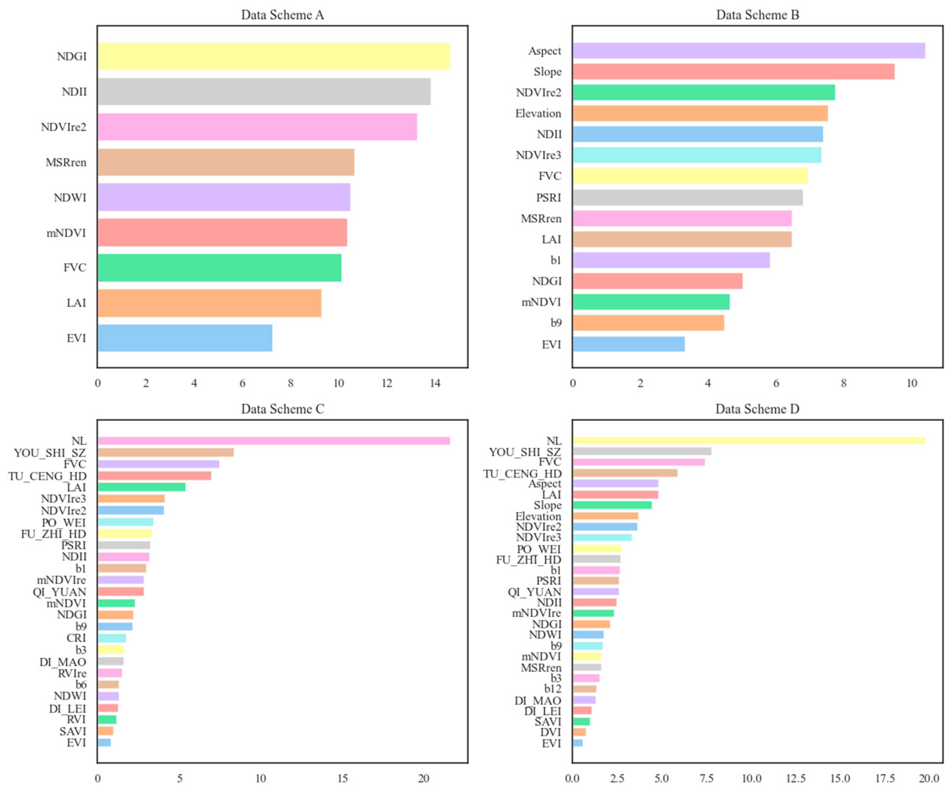
3.1. Feature Selection

The Recursive Feature Elimination with Cross-Validation (RFECV) algorithm was employed for dimensionality reduction of the indicator set, using the CatBoost algorithm as the base processor for feature selection. The algorithm parameters were carefully finetuned, designating kappa as the scoring function, and repeated validation was achieved through the 10-fold cross-validation utilized.

As shown in Table 11, we devised four distinct data schemes (A, B, C, and D) for modeling, each encompassing a unique combination of data. After conducting feature importance analysis using CatBoost, the specific significance of each feature factor was ultimately revealed, as illustrated in Figure 7. The figure suggests that the average tree age (NL) and dominant tree species (YOU_SHI_SZ) play a pivotal role in forest structure assessment.

After that, by leveraging the RFECV algorithm, we selected the feature factors from these schemes; the detailed results are outlined in

Table 13. Selected factors for four data schemes using RFECV algorithm.

Factors	A	B	C	D	Factors	A	B	C	D
b1		√	√	√	NDII	√	√	√	√
b3			√	√	mNDVI	√	√	√	√
b6			√		RVIre			√
b9		√	√	√	LAI	√	√	√	√
b12				√	FVC	√	√	√	√
CRI			√		Elevation	-	√	-	√
MSRren	√	√		√	Aspect	-	√	-	√
PSRI		√	√	√	Slope	-	√	-	√
NDVIre2	√	√	√	√	DI_LEI	-	-	√	√
NDVIre3		√	√	√	DI_MAO	-	-	√	√
RVI			√		PO_WEI	-	-	√	√
NDWI	√		√	√	TU_CENG_HD	-	-	√	√
mNDVIre			√	√	FU_ZHI_HD	-	-	√	√
SAVI			√	√	QI_YUAN	-	-	√	√
DVI				√	YOU_SHI_SZ	-	-	√	√
EVI	√	√	√	√	NL	-	-	√	√
NDGI	√	√	√	√

.

3.2. Comparative Analysis of Classification Results

Table 14. Performance of four models based on four data schemes.

Program	Overall Accuracy Rate	Category Accuracy Rate			Recall	Kappa
		Good	Moderate	Poor
KNN-A	75.33%	50.43%	79.36%	47.99%	48.27%	0.2538
KNN-B	75.23%	48.99%	79.78%	49.17%	49.69%	0.2701
KNN-C	82.24%	67.08%	85.39%	69.96%	65.14%	0.5108
KNN-D	81.87%	65.85%	84.91%	70.57%	63.86%	0.4954
SVM-A	76.41%	66.01%	76.85%	63.11%	38.96%	0.1208
SVM-B	77.26%	69.06%	77.90%	64.17%	42.61%	0.1918
SVM-C	84.54%	74.82%	86.86%	74.12%	69.00%	0.5751
SVM-D	84.48%	75.62%	86.90%	72.81%	69.09%	0.5749
RF-A	77.58%	66.20%	79.26%	56.01%	47.42%	0.2664
RF-B	77.81%	67.78%	79.22%	58.23%	47.19%	0.2659
RF-C	86.20%	76.48%	87.84%	81.34%	71.52%	0.6203
RF-D	86.33%	77.79%	87.72%	82.08%	71.24%	0.6209
CatBoost-A	77.41%	62.10%	79.91%	54.55%	49.71%	0.2936
CatBoost-B	77.51%	60.47%	79.96%	57.23%	49.79%	0.2959
CatBoost-C	87.75%	77.52%	89.91%	81.53%	76.52%	0.6756
CatBoost-D	88.07%	78.19%	90.04%	82.82%	76.86%	0.6833

presents the experimental results for the SVM, KNN, RF, and CatBoost algorithms, based on four distinct data schemes. Initially, Data Scheme A, comprised solely of single-source remote sensing data (including Sentinel-2 original bands, vegetation index, LAI, and FVC), yielded the least effective performance, with overall accuracies ranging between 75.33% and 77.58% across the four models. Subsequently, Data Scheme B, which combined single-source remote sensing data with terrain features derived from DEMs data, resulted in an overall accuracy improvement for all the models, except for a slight decrease of 0.1% in the KNN. The CatBoost, RF, and SVM algorithms improved the performance by 0.10%, 0.23%, and 0.85%, respectively. Data Scheme C, which combined single-source remote sensing data with field survey data, significantly improved the model’s performance, boosting the overall accuracy by 6.91% to 10.34%. Data Scheme D, encompassing all previously mentioned data, that is, single-source remote sensing data, terrain features, and field survey data, emerged with the best performance, with overall accuracies ranging from 86.33% to 88.07% across the four distinct models. Furthermore, the accuracies for the categories “good”, “moderate”, and “poor” were 70.57% to 82.82%, 84.91% to 90.04%, and 65.85% to 78.19%, respectively, accompanied by a kappa coefficient that ranged from 0.4954 to 0.6833. In summary, the integration of multiple data sources, particularly the inclusion of field survey data, substantially improved the accuracy of the forest structure classification. While Data Scheme D excelled in regard to ensemble learning algorithms like RF and CatBoost, Data Scheme C was superior in regard to traditional classifiers, such as KNN and SVM. In terms of algorithms, the experimental results showed that ensemble learning algorithms have higher prediction accuracy and reliability than traditional classifiers. Specifically, in regard to Data Scheme D, RF’s kappa coefficient increased by 0.1255 compared to KNN and by 0.046 compared to SVM, while CatBoost further improved by 0.0624 based on RF. The overall accuracy of RF was 4.46% higher than KNN and 1.85% higher than SVM, while CatBoost further improved by 1.74% based on RF. These insights offer valuable guidance for future research and applications in regard to forest structure classification.

Furthermore, the CatBoost model consistently outperformed all the data schemes, achieving remarkable results in the CatBoost Data Scheme D model, specifically. The model achieved an impressive overall accuracy of 88.07%, along with a recall of 76.86%, and a kappa coefficient of 0.6833. These results indicated that the CatBoost model has high accuracy and stability in addressing forest structure classification challenges.

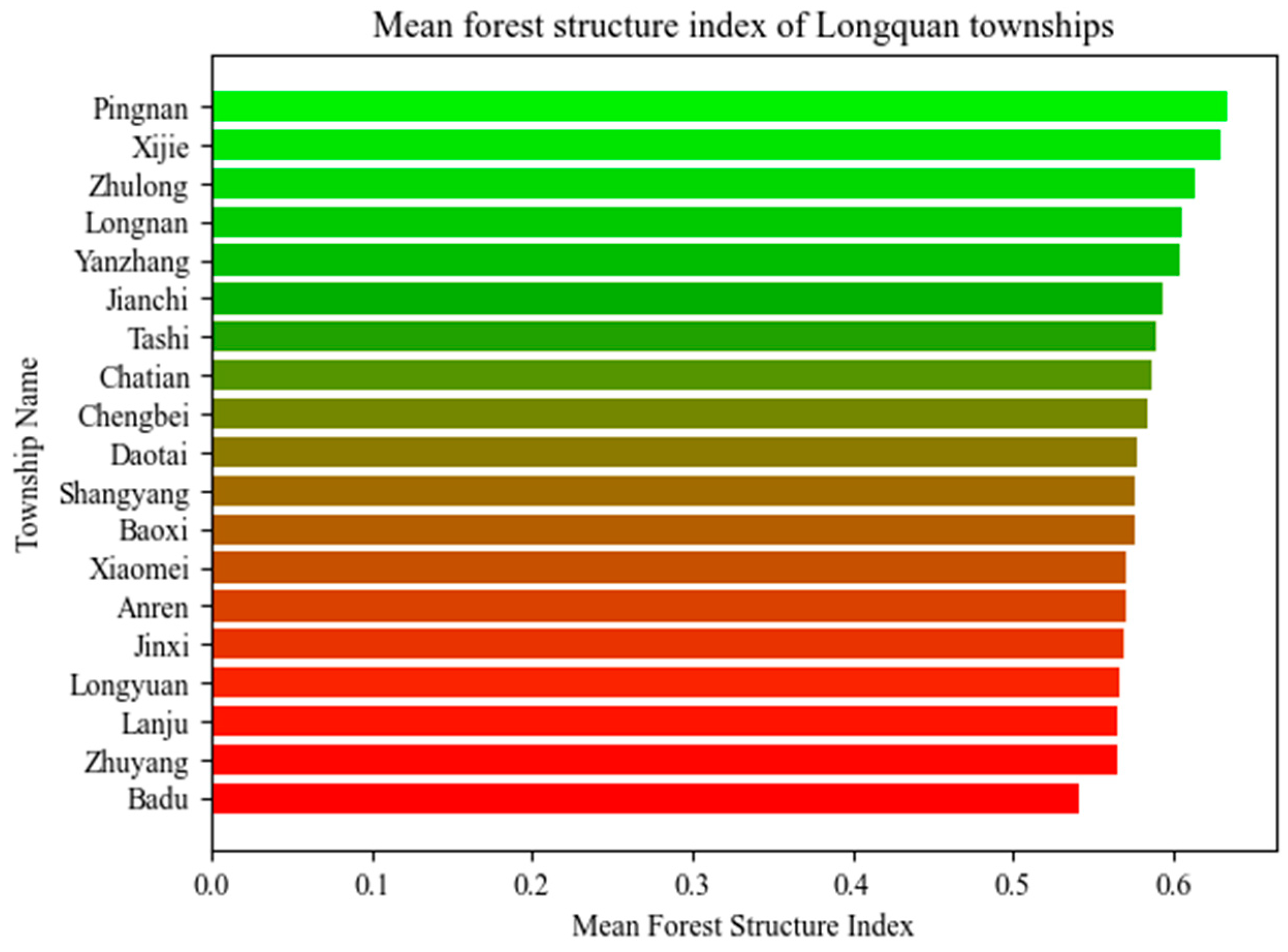
3.3. Results on the Forest Structure Grades in Longquan City

Ultimately, the levels of forest structure grades for Longquan City were evaluated based on Data Scheme D and the CatBoost algorithm, and the results are presented in

Table 15. Results of forest structural classifications.

Level	Longquan City
	Sub-Compartment Quantity	Percentage
Good	6273	11.18%
Moderate	43,070	76.77%
Poor	6757	12.05%

. Among the 56,100 sub-compartments, the majority belonged to the “moderate” forest structure level, with a total of 43,070, accounting for 76.77% of the entire dataset. In contrast, there were much fewer levels classified as “poor”, with a total of only 6757, accounting for 12.05% of the total. Finally, the least prevalent category was the sub-compartments with a “good” level of forest structure, totaling 6273 and accounting for 11.18% of the overall data.

Figure 8 presents the levels of forest structure grades for the forest sub-compartments in Longquan City. Meanwhile, Figure 9 illustrates the average FSI for various townships in Longquan City, highlighting the Pingnan Township and Xijie Street as the areas with the most favorable forest structure. This is primarily attributable to the Fengyang Mountain National Nature Reserve in Pingnan Township and the expansive forest area in Xijie Street. Conversely, the Batu Township exhibited the least desirable forest structure level. Despite the fact that Batu Town is known as “the premier town in Longquan City”, the area of pure forest accounts for 59% of the total forest area, which may lead to a lower FSI.

4. Discussion

4.1. Remote Sensing in Forest Structure Evaluation

This study computed 22 vegetation indices for assessing forest structure, using Sentinel-2 imagery. These indices span multiple aspects, ranging from spectral reflectance to vegetation structure, and included well-known metrics, such as RVI, NDVI, DVI, EVI, and SAVI, which mirror crucial forest parameters, such as forest biomass, growth status, and vegetation cover [50].

Using the CatBoost algorithm as the base processor for feature selection, the RFECV algorithm was further used to extract the key remote sensing factors that significantly impact forest structure classification. These selected factors are statistically significant and intimately tied to the anticipated changes in forest structure parameters. For instance, the PSRI is closely linked to the health of forests, while the NDII is correlated with forest growth conditions. Furthermore, the combination of NDII and NDGI effectively captures the phenological information of vegetation [51], offering a nuanced understanding of its seasonal fluctuations. Additionally, the SAVI and NDWI shed light on forests’ water use efficiency and drought stress, respectively [52,53]. By integrating diverse remote sensing information, we can facilitate a comprehensive forest structure assessment across multiple dimensions. However, to achieve a more precise evaluation, it is imperative to combine these remote sensing data with ground survey data. This integration yields a richer and more accurate information set that is invaluable for forest management and ecological research, enabling more informed decision-making and effective conservation strategies.

Currently, the integration of multi-source remote sensing data with machine learning for the assessment of forest structure remains an under-explored area. This manuscript presents a novel approach to evaluating forest structure, considering aspects such as the tree species composition, tree age, and the spatial structure of forests. By utilizing remote sensing data and easily obtainable ground survey data, machine learning techniques are applied to evaluate the forest structure, significantly reducing the need for extensive manual measurements. Similar methodologies have been employed in previous studies to assess forest ecological functions [20].

4.2. Complementarity of Multi-Source Data

Integrating multiple data sources can effectively offset the limitations inherent in different datasets [54]. Data Scheme A, which relied exclusively on Sentinel-2 optical remote sensing data, demonstrated limited effectiveness in classifying forest structure levels. Principally, the evaluation of forest structure necessitates ten forest parameters, most of which cannot be inverted using only optical remote sensing data [55,56]. For instance, predicting the tree age group structure, mean diameter at breast height, and mean tree height, using solely optical remote sensing data, has yielded unsatisfactory results. Nevertheless, the integration of multiple data sources can effectively compensate for the deficiencies of optical remote sensing by inverting specific forest parameters [57].

Consequently, this study supplemented DEMs and field survey data based on optical remote sensing to identify the optimal data scheme. Upon comparison, it was determined that Data Scheme D, which integrated remote sensing images, DEMs, and field survey data, performed optimally in regard to the ensemble learning algorithms, achieving an impressive overall accuracy, ranging from 86.33% to 88.07%. The inclusion of DEM data provided the critical terrain features lacking in optical remote sensing, thereby helping to estimate the average tree height [58,59,60]. Furthermore, the tree age in the field survey data positively correlated with most of the forest structural parameters, such as the mean diameter at breast height, mean tree height, and tree age group structure [61]. By employing this method, the model facilitates more convenient long-term monitoring, leading to a more profound understanding of the dynamic changes in the forest structure. Moreover, these factors are often readily available through remote sensing images or straightforward on-site surveys, greatly simplifying the complexity of field investigations and reducing associated costs.

4.3. Advantages of CatBoost

This study aimed to identify the optimal machine learning algorithm for assessing forest structure by integrating multiple data sources. The RFECV selection method was utilized to deal with the intricate relationships between feature factors in high-dimensional data, enhancing the model’s flexibility and processing speed. Notably, most indicators, including ground survey factors and spectral features, exhibited nonlinear relationships with forest structure indices. For instance, as the tree age increased, the forest structure indices initially climbed and then declined, highlighting the intricate nature of their interplay beyond mere linear connections. Consequently, the study deployed the CatBoost algorithm, amplifying the objective function’s nonlinear approximation and improving the prediction accuracy. Among all the data schemes, the CatBoost algorithm exhibited the highest kappa coefficient, with values ranging from 0.2936 to 0.6833, and demonstrated remarkable proficiency in handling large-scale data. The underlying algorithm, rooted in symmetric binary trees to compute leaf nodes, accelerated model training and inference. Furthermore, the CatBoost algorithm’s inherent ability to account for missing values during decision tree construction obviated the need for additional preprocessing steps, streamlining data processing and enhancing the model’s robustness [62].

Moreover, the CatBoost algorithm can autonomously determine the importance of variables, thereby augmenting the accuracy and usability of the model. Researchers that combine field survey data with remote sensing data have demonstrated significant advancements using the CatBoost algorithm to estimate forest biomass or assess forest quality [63,64]. Moreover, we posit that the CatBoost algorithm is a promising methodology for establishing forest structure assessment models using remote sensing data, meriting deeper exploration and broader implementation.

4.4. Limitations of This Study

In this study, we exclusively employed the RFECV algorithm, with the CatBoost algorithm as the base estimator for feature extraction. However, it is worth exploring other algorithms or alternative feature selection methods to broaden our perspective. Our future research aims to conduct comparative analyses of multiple feature selection methods.

The ecosystem under scrutiny exhibits a significant imbalance in the hierarchical distribution of the forest structure. This data imbalance could compromise the accuracy and reliability of our models. To uphold the validity of our research findings, it is crucial to devise and implement more suitable strategies to counteract this imbalance. Our subsequent research phase will tackle this data imbalance, focusing on the improvement of data preprocessing algorithms and estimation models.

The forest structure offers a comprehensive perspective on forest space utilization. The forest structure assessment incorporates horizontal factors, like canopy density and leaf area index, and vertically distributed factors, such as tree height and forest layer. Future studies could utilize radar remote sensing to more accurately reflect the vertical distribution of forests in space, thereby enhancing the performance of our model.

5. Conclusions

This study refers to the forest ecological quality monitoring index system and technical specifications to compute the forest structure indices specific to Longquan City sub-compartments and, subsequently, categorize them as good, moderate, or poor. Among the 56,100 sub-compartments after preprocessing, the majority belonged to the “moderate” forest structure level, with a total of 43,070, accounting for 76.77% of the entire dataset.

By integrating multiple data sources, including Sentinel-2 remote sensing data, DEMs, and field survey data, the inherent limitations of the different datasets are effectively offset, resulting in optimal performance.

The application of the RFECV method has been proven to be effective in eliminating irrelevant factors, reducing data dimensionality and, subsequently, enhancing the model’s generalizability. The screening results show that the average tree age and dominant tree species are the most significant factors.

Among the four machine learning algorithms, the CatBoost algorithm emerged as the most accurate and stable model across all datasets, achieving a kappa coefficient of 0.6833, an overall accuracy rate of 88.07%, and a recall rate of 76.86%.

By utilizing remote sensing data, DEMs, and easily obtainable ground survey data, machine learning algorithms are applied to evaluate forest structure, significantly reducing the cost of data surveys.

References

1. Mason, B.; Mencuccini, M. Managing Forests for Ecosystem Services—Can Spruce Forests Show the Way? Forestry 2014, 87, 189–191. [Google Scholar] [CrossRef]
2. Staudhammer, C.L.; LeMay, V.M. Introduction and Evaluation of Possible Indices of Stand Structural Diversity. Can. J. For. Res. 2001, 31, 1105–1115. [Google Scholar] [CrossRef]
3. Franklin, J.F.; Spies, T.A.; Pelt, R.V.; Carey, A.B.; Thornburgh, D.A.; Berg, D.R.; Lindenmayer, D.B.; Harmon, M.E.; Keeton, W.S.; Shaw, D.C.; et al. Disturbances and Structural Development of Natural Forest Ecosystems with Silvicultural Implications, Using Douglas-Fir Forests as an Example. For. Ecol. Manag. 2002, 155, 399–423. [Google Scholar] [CrossRef]
4. Scrinzi, G.; Marzullo, L.; Galvagni, D. Development of a Neural Network Model to Update Forest Distribution Data for Managed Alpine Stands. Ecol. Model. 2007, 206, 331–346. [Google Scholar] [CrossRef]
5. Liang, X.; Kukko, A.; Hyyppä, J.; Lehtomäki, M.; Pyörälä, J.; Yu, X.; Kaartinen, H.; Jaakkola, A.; Wang, Y. In-Situ Measurements from Mobile Platforms: An Emerging Approach to Address the Old Challenges Associated with Forest Inventories. ISPRS J. Photogramm. Remote Sens. 2018, 143, 97–107. [Google Scholar] [CrossRef]
6. GB/T 26424-2010; Technical Regulations for Inventory for Forest Management Planning and Design. Survey, Planning and Design Institute of the State Forestry Administration: Beijing, China, 2011; p. 56.
7. Meng, Y.; Cao, B.; Dong, C.; Dong, X. Mount Taishan Forest Ecosystem Health Assessment Based on Forest Inventory Data. Forests 2019, 10, 657. [Google Scholar] [CrossRef]
8. Liu, Z.; Wu, Y.; Zhang, X.; Li, M.; Liu, C.; Li, W.; Fu, M.; Qin, S.; Fan, Q.; Luo, H.; et al. Comparison of Variable Extraction Methods Using Surface Field Data and Its Key Influencing Factors: A Case Study on Aboveground Biomass of Pinus Densata Forest Using the Original Bands and Vegetation Indices of Landsat 8. Ecol. Indic. 2023, 157, 111307. [Google Scholar] [CrossRef]
9. Immitzer, M.; Atzberger, C.; Koukal, T. Tree Species Classification with Random Forest Using Very High Spatial Resolution 8-Band WorldView-2 Satellite Data. Remote Sens. 2012, 4, 2661–2693. [Google Scholar] [CrossRef]
10. Zhu, L.; Zhou, S. Research on automatic estimation method of forest canopy based on spatial data cloud platform and machine learning. For. Constr. 2018, 31–34. [Google Scholar]
11. Periasamy, S.; Ravi, K.P. A Novel Approach to Quantify Soil Salinity by Simulating the Dielectric Loss of SAR in Three-Dimensional Density Space. Remote Sens. Environ. 2020, 251, 112059. [Google Scholar] [CrossRef]
12. Feng, Q.; Zhou, L.; Chen, E.; Liang, X.; Zhao, L.; Zhou, Y. The Performance of Airborne C-Band PolInSAR Data on Forest Growth Stage Types Classification. Remote Sens. 2017, 9, 955. [Google Scholar] [CrossRef]
13. TAN, P.; ZHU, J.; FU, H.; LIN, H. Inversion of Forest Height Based on ALOS-2 PARSAR-2 Multi-Baseline Polarimetric SAR Interferometry Data. J. Radars 2020, 9, 569–577. [Google Scholar]
14. Zhang, Y.; Li, M. A New Method for Monitoring Start of Season (SOS) of Forest Based on Multisource Remote Sensing. Int. J. Appl. Earth Obs. Geoinf. 2021, 104, 102556. [Google Scholar] [CrossRef]
15. Roffey, M.; Wang, J. Evaluation of Features Derived from High-Resolution Multispectral Imagery and LiDAR Data for Object-Based Support Vector Machine Classification of Tree Species. Can. J. Remote Sens. 2020, 46, 473–488. [Google Scholar] [CrossRef]
16. Kumar, P.; Krishna, A.P. InSAR-Based Tree Height Estimation of Hilly Forest Using Multitemporal Radarsat-1 and Sentinel-1 SAR Data. IEEE J. Sel. Top. Appl. Earth Obs. Remote Sens. 2019, 12, 5147–5152. [Google Scholar] [CrossRef]
17. Ahmed, O.S.; Franklin, S.E.; Wulder, M.A.; White, J.C. Characterizing Stand-Level Forest Canopy Cover and Height Using Landsat Time Series, Samples of Airborne LiDAR, and the Random Forest Algorithm. ISPRS J. Photogramm. Remote Sens. 2015, 101, 89–101. [Google Scholar] [CrossRef]
18. Panagiotidis, D.; Abdollahnejad, A.; Slavík, M. 3D Point Cloud Fusion from UAV and TLS to Assess Temperate Managed Forest Structures. Int. J. Appl. Earth Obs. Geoinf. 2022, 112, 102917. [Google Scholar] [CrossRef]
19. Ette, J.S.; Ritter, T.; Vospernik, S. Insights in Forest Structural Diversity Indicators with Machine Learning: What Is Indicated? Biodivers. Conserv. 2023, 32, 1019–1046. [Google Scholar] [CrossRef]
20. Fang, N.; Yao, L.; Wu, D.; Zheng, X.; Luo, S. Assessment of Forest Ecological Function Levels Based on Multi-Source Data and Machine Learning. Forests 2023, 14, 1630. [Google Scholar] [CrossRef]
21. Gebauer, A.; Brito Gómez, V.M.; Ließ, M. Optimisation in Machine Learning: An Application to Topsoil Organic Stocks Prediction in a Dry Forest Ecosystem. Geoderma 2019, 354, 113846. [Google Scholar] [CrossRef]
22. Huang, X. Research and Development of Feature Dimensionality Reduction. Comput. Sci. 2018, 45, 16-21+53. [Google Scholar]
23. Jeon, H.; Oh, S. Hybrid-Recursive Feature Elimination for Efficient Feature Selection. Appl. Sci. 2020, 10, 3211. [Google Scholar] [CrossRef]
24. Shen, Z.; Miao, J.; Wang, J.; Zhao, D.; Tang, A.; Zhen, J. Evaluating Feature Selection Methods and Machine Learning Algorithms for Mapping Mangrove Forests Using Optical and Synthetic Aperture Radar Data. Remote Sens. 2023, 15, 5621. [Google Scholar] [CrossRef]
25. T/CSF 002-2021; Monitoring Indicator System and Technological Specification of Forest Ecological Quality. Ecology and Nature Conservation Institute, Chinese Academy of Forestry: Beijing, China, 2021; pp. 5–14.
26. Raiyani, K.; Gonçalves, T.; Rato, L.; Salgueiro, P.; Marques Da Silva, J.R. Sentinel-2 Image Scene Classification: A Comparison between Sen2Cor and a Machine Learning Approach. Remote Sens. 2021, 13, 300. [Google Scholar] [CrossRef]
27. Rouse, J.W.; Haas, R.H.; Schell, J.A.; Deering, D.W. Monitoring Vegetation Systems in the Great Plains with ERTS. NASA Spec. Publ. 1973, 351, 309. [Google Scholar]
28. Jordan, C.F. Derivation of Leaf-Area Index from Quality of Light on the Forest Floor. Ecology 1969, 50, 663–666. [Google Scholar] [CrossRef]
29. Hardisky, M.A. The Influence of Soil Salinity, Growth Form, and Leaf Moisture on-the Spectral Radiance of Spartina alterniflora Canopies. Photogramm. Eng. Remote Sens. 1983, 49, 77–83. [Google Scholar]
30. Yang, W.; Kobayashi, H.; Wang, C.; Shen, M.; Chen, J.; Matsushita, B.; Tang, Y.; Kim, Y.; Bret-Harte, M.S.; Zona, D.; et al. A Semi-Analytical Snow-Free Vegetation Index for Improving Estimation of Plant Phenology in Tundra and Grassland Ecosystems. Remote Sens. Environ. 2019, 228, 31–44. [Google Scholar] [CrossRef]
31. Huete, A.R.; Liu, H.Q.; Batchily, K.; van Leeuwen, W. A Comparison of Vegetation Indices over a Global Set of TM Images for EOS-MODIS. Remote Sens. Environ. 1997, 59, 440–451. [Google Scholar] [CrossRef]
32. Richardson, A.J.; Wiegand, C.L. Distinguishing Vegetation from Soil Background Information. Photogramm. Eng. Remote Sens. 1977, 43, 1541–1552. [Google Scholar]
33. Huete, A.R. A Soil-Adjusted Vegetation Index (SAVI). Remote Sens. Environ. 1988, 25, 295–309. [Google Scholar] [CrossRef]
34. Lopez-Alvarez, B.; Urbano-Peña, M.A.; Moran-Ramírez, J.; Ramos-Leal, J.A.; Tuxpan-Vargas, J. Estimation of the Environment Component of the Water Poverty Index via Remote Sensing in Semi-Arid Zones. Hydrol. Sci. J. 2020, 65, 2647–2657. [Google Scholar] [CrossRef]
35. Liu, L.; Pang, Y.; Ren, H.; Li, Z. Predict Tree Species Diversity from GF-2 Satellite Data in a Subtropical Forest of China. Sci. Silvae Sin. 2019, 55, 61–74. [Google Scholar]
36. Sims, D.; Gamon, J. Relationships Between Leaf Pigment Content and Spectral Reflectance Across a Wide Range of Species, Leaf Structures and Developmental Stages. Remote Sens. Environ. 2002, 81, 337–354. [Google Scholar] [CrossRef]
37. Zong, Y.; Li, Y.; Liu, H. A Study of Coastal Wetland Vegetation Classification Based on Object⁃oriented Random Forest Method. J. Nanjing Norm. Univ. (Eng. Technol. Ed.) 2021, 47–55. [Google Scholar]
38. Cao, L. Estimation of Forest Stock Volume in Yanqing District Based on Sentinel-2 Images; Beijing Forestry University: Beijing, China, 2019. [Google Scholar]
39. Gitelson, A.A.; Merzlyak, M.N. Remote Estimation of Chlorophyll Content in Higher Plant Leaves. Int. J. Remote Sens. 1997, 18, 2691–2697. [Google Scholar] [CrossRef]
40. Zhang, X.; Hou, X.; Wang, M.; Wang, L.; Liu, F. Study on Relationship Between Photosynthetic Rate and Hyperspectral Indexes of Wheat Under Stripe Rust Stress. Spectrosc. Spectr. Anal. 2022, 42, 940–946. [Google Scholar]
41. Wang, X. Research on Forest Dynamic Change Detection Method Based on Sentinel-2; Huazhong Agricultural University: Wuhan, China, 2020. [Google Scholar]
42. De Luca, G.; MN Silva, J.; Di Fazio, S.; Modica, G. Integrated Use of Sentinel-1 and Sentinel-2 Data and Open-Source Machine Learning Algorithms for Land Cover Mapping in a Mediterranean Region. Eur. J. Remote Sens. 2022, 55, 52–70. [Google Scholar] [CrossRef]
43. Wang, B.; Wang, W.; Zhou, C.; Fang, Y.; Zheng, Y. Feature Selection and Classification of Heart Sound Based on EMD Adaptive Reconstruction. Space Med. Med. Eng. 2020, 33, 533–541. [Google Scholar] [CrossRef]
44. Lu, P.; Zhuo, Z.; Zhang, W.; Tang, J.; Wang, Y.; Zhou, H.; Huang, X.; Sun, T.; Lu, J. A Hybrid Feature Selection Combining Wavelet Transform for Quantitative Analysis of Heat Value of Coal Using Laser-Induced Breakdown Spectroscopy. Appl. Phys. B 2021, 127, 19. [Google Scholar] [CrossRef]
45. Zhang, Y.; Zhao, Z.; Zheng, J. CatBoost: A New Approach for Estimating Daily Reference Crop Evapotranspiration in Arid and Semi-Arid Regions of Northern China. J. Hydrol. 2020, 588, 125087. [Google Scholar] [CrossRef]
46. Huang, G.; Wu, L.; Ma, X.; Zhang, W.; Fan, J.; Yu, X.; Zeng, W.; Zhou, H. Evaluation of CatBoost Method for Prediction of Reference Evapotranspiration in Humid Regions. J. Hydrol. 2019, 574, 1029–1041. [Google Scholar] [CrossRef]
47. Jiang, Q.; Yang, X.; Yang, C.; Zhao, Z. Object-Oriented Land Use Classification Based on CatBoost Algorithm. J. Jilin Univ. (Inf. Sci. Ed.) 2020, 38, 185–191. [Google Scholar]
48. Pedregosa, F.; Varoquaux, G.; Gramfort, A.; Michel, V.; Thirion, B.; Grisel, O.; Blondel, M.; Müller, A.; Nothman, J.; Louppe, G.; et al. Scikit-Learn: Machine Learning in Python. J. Mach. Learn. Res. 2011, 12, 2825–2830. [Google Scholar]
49. Prokhorenkova, L.; Gusev, G.; Vorobev, A.; Dorogush, A.V.; Gulin, A. CatBoost: Unbiased Boosting with Categorical Features. Adv. Neural Inf. Process. Syst. 2019, 31, 1–11. [Google Scholar]
50. Hussain, S.; Raza, A.; Abdo, H.G.; Mubeen, M.; Tariq, A.; Nasim, W.; Majeed, M.; Almohamad, H.; Al Dughairi, A.A. Relation of Land Surface Temperature with Different Vegetation Indices Using Multi-Temporal Remote Sensing Data in Sahiwal Region, Pakistan. Geosci. Lett. 2023, 10, 33. [Google Scholar] [CrossRef]
51. Xu, J.; Tang, Y.; Xu, J.; Chen, J.; Bai, K.; Shu, S.; Yu, B.; Wu, J.; Huang, Y. Evaluation of Vegetation Indexes and Green-Up Date Extraction Methods on the Tibetan Plateau. Remote Sens. 2022, 14, 3160. [Google Scholar] [CrossRef]
52. Bagheri, N. Application of Aerial Remote Sensing Technology for Detection of Fire Blight Infected Pear Trees. Comput. Electron. Agric. 2020, 168, 105147. [Google Scholar] [CrossRef]
53. Pérez-Romero, J.; Navarro-Cerrillo, R.M.; Palacios-Rodriguez, G.; Acosta, C.; Mesas-Carrascosa, F.J. Improvement of Remote Sensing-Based Assessment of Defoliation of Pinus Spp. Caused by Thaumetopoea Pityocampa Denis and Schiffermüller and Related Environmental Drivers in Southeastern Spain. Remote Sens. 2019, 11, 1736. [Google Scholar] [CrossRef]
54. Lin, H.; Liu, X.; Han, Z.; Cui, H.; Dian, Y. Identification of Tree Species in Forest Communities at Different Altitudes Based on Multi-Source Aerial Remote Sensing Data. Appl. Sci. 2023, 13, 4911. [Google Scholar] [CrossRef]
55. Spracklen, B.; Spracklen, D.V. Synergistic Use of Sentinel-1 and Sentinel-2 to Map Natural Forest and Acacia Plantation and Stand Ages in North-Central Vietnam. Remote Sens. 2021, 13, 185. [Google Scholar] [CrossRef]
56. Fang, G.; Xu, H.; Yang, S.-I.; Lou, X.; Fang, L. Synergistic Use of Sentinel-1, Sentinel-2, and Landsat 8 in Predicting Forest Variables. Ecol. Indic. 2023, 151, 110296. [Google Scholar] [CrossRef]
57. Ahmadi, K.; Kalantar, B.; Saeidi, V.; Harandi, E.K.G.; Janizadeh, S.; Ueda, N. Comparison of Machine Learning Methods for Mapping the Stand Characteristics of Temperate Forests Using Multi-Spectral Sentinel-2 Data. Remote Sens. 2020, 12, 3019. [Google Scholar] [CrossRef]
58. He, W.; Zhu, J.; Lopez-Sanchez, J.M.; Gómez, C.; Fu, H.; Xie, Q. Forest Height Inversion by Combining Single-Baseline TanDEM-X InSAR Data with External DTM Data. Remote Sens. 2023, 15, 5517. [Google Scholar] [CrossRef]
59. Xia, Y.; Pang, Y.; Liu, L.; Chen, B.; Dong, B.; Huang, Q. Forest Height Growth Monitoring of Cunninghamia lanceolata Plantation Using Multi-Temporal Aerial Photography with the Support of High Accuracy DEM. Sci. Silvae Sin. 2019, 55, 108–121. [Google Scholar]
60. Shen, J.; Lei, X.; Li, Y.; Lan, Y. Prediction mean height for Larix olgensis plantation based on Bayesian-regularization BP neural network. J. Nanjing For. Univ. 2018, 42, 147–154. [Google Scholar]
61. Rajarajan, K.; Verma, S.; Sahu, S.; Radhakrishna, A.; Kumar, N.; Priyadarshini, E.; Handa, A.; Arunachalam, A. Differential Gene Expression Analysis Reveals the Fast-Growth Mechanisms in Melia Dubia at Different Stand Ages. Mol. Biol. Rep. 2023, 50, 10671–10675. [Google Scholar] [CrossRef]
62. Hancock, J.T.; Khoshgoftaar, T.M. CatBoost for Big Data: An Interdisciplinary Review. J. Big Data 2020, 7, 94. [Google Scholar] [CrossRef] [PubMed]
63. Cao, L.; He, X.; Chen, S.; Fang, L. Assessing Forest Quality through Forest Growth Potential, an Index Based on Improved CatBoost Machine Learning. Sustainability 2023, 15, 8888. [Google Scholar] [CrossRef]
64. Zhang, Y.; Ma, J.; Liang, S.; Li, X.; Li, M. An Evaluation of Eight Machine Learning Regression Algorithms for Forest Aboveground Biomass Estimation from Multiple Satellite Data Products. Remote Sens. 2020, 12, 4015. [Google Scholar] [CrossRef]
Figure 1. (A) Administrative distribution map of China; (B) administrative distribution map of Zhejiang Province; (C) township administrative distribution map of Longquan City.
Forests 15 00533 g001
Figure 2. Schematic framework.
Forests 15 00533 g002
Figure 3. DEM image of Longquan City.
Forests 15 00533 g003
Figure 4. (A) Sentinel-2 optical remote sensing image of Longquan City; (B) schematic diagram of sub-compartment.
Forests 15 00533 g004
Figure 5. Calculation results on the forest structure index in Longquan City.
Forests 15 00533 g005
Figure 6. RFECV method workflow figure.
Forests 15 00533 g006
Figure 7. Importance of CatBoost features for four data schemes.
Forests 15 00533 g007
Figure 8. Levels of forest structure grades in Longquan City.
Forests 15 00533 g008
Figure 9. FSI ranking for various towns in Longquan City.
Forests 15 00533 g009