Abstract
Exposure to green spaces (GSs) has been perceived as a natural and sustainable solution to urban challenges, playing a vital role in rapid urbanization. Previous studies, due to their lack of direct spatial alignment and attention to a human-scale perspective, struggled to comprehensively measure urban GS exposure. To address this gap, our study introduces a novel GS exposure assessment framework, employing machine learning and street view images. We conducted a large-scale, fine-grained empirical study focused on downtown Shanghai. Our findings indicate a pronounced hierarchical structure in the distribution of GS exposure, which initially increases and subsequently decreases as one moves outward from the city center. Further, from both the micro and macro perspectives, we employed structural equation modeling and Geodetector to investigate the impact of the urban built environment on GS exposure. Our results highlight that maintaining an appropriate level of architectural density, enhancing the combination of sidewalks with GSs, emphasizing the diversity of regional characteristics, and avoiding excessive concentration of functions are effective approaches for increasing urban GS exposure and promoting human wellbeing. Our study offers scientific insights for urban planners and administrators, holding significant implications for achieving sustainable urban development.
1. Introduction
Urban green spaces (GSs), as the sole natural elements within urban structures, play a pivotal role in residents’ daily lives. They provide a range of services, including mitigating urban heat island effects [1], promoting urban hydrological cycles [2], enhancing biodiversity [3], and improving air quality [4]. Presently, rapid urbanization processes lead to chaotic urban expansion, population surges, and increased construction [5,6]. With escalating urban challenges and human habitats being at risk, urban GSs arise as nature-based, sustainable solutions [7,8]. This situation compels urban managers, planners, and researchers to reassess urban GSs, emphasizing their benefits to humanity [9].
GS exposure is typically defined as the extent of an individual’s (or group’s) interactions with natural settings [10]. This directly affects the health impacts of GSs on urban residents, making GS exposure a burgeoning interdisciplinary research area. There are various advantages of GS exposure [11,12]. On the one hand, GSs provide recreational areas, promoting outdoor exercise and physical health [13,14]. On the other hand, they can directly enhance residents’ mood, alleviate stress, restore focus, and, consequently, diminish the onset of disorders like depression [15,16,17]. The global trend of increasingly high population concentrations in urban areas is intensifying [18]. The exposure to GSs in the streets or at small scales heavily influences the daily lives of residents and is crucial in improving environmental quality. Such small-scale renewal and enhancement are also major aspects of future urban planning and construction [19,20]. Therefore, it is necessary to measure GS exposure at the street level to improve residents’ wellbeing.
Early research in environmental science and ecology focused on the significance of the natural environment for human society, emphasizing the protection of biodiversity, ecosystem services, and natural resources [21]. With the development of public health science, attention began to shift towards the impact of GSs on human health, such as improving the water quality, regulating microclimates, and purifying air [22,23]. Furthermore, psychological research has found that GSs have a positive impact on individuals’ mental health and emotional wellbeing, with the potential benefits of this impact even surpassing other aspects of greenery. Studies have shown that more GSs in people’s living environments are associated with enhanced social security, which helps improve their mental health [24]. With the acceleration of urbanization, people’s expectations for the quality of urban life have gradually increased, thereby focusing more attention on urban GSs as a part of residents’ daily lives [25,26]. In addition, the impact of urban GSs on residents has attracted further interest from scholars [15]. In this process, the concept of “GS exposure” was gradually proposed to describe the extent of people’s contact with GSs in their daily lives [10]. This concept quickly gained recognition in the academic community and was explored as a novel perspective on the relationship between humans and nature. Gong et al. argue that the positive effects of GS exposure are significant for vulnerable groups, such as children and the elderly [27]. Zhang et al. categorize the impact of GSs on residents’ health into three pathways: reducing harmful exposures, psychological restoration, and encouraging health-related behaviors [28]. Numerous studies have also combined GS exposure with epidemiological investigations, revealing the potential of GS exposure assessments in public health research [29,30].
The measurement of GS exposure is a foundational aspect of this area of research. The method of calculating GS exposure based on processing remote sensing data using GIS platforms has been widely used in previous research [31]. The Normalized Difference Vegetation Index (NDVI) can be used to measure the spatial distribution of urban greenery; therefore, it is often used as an important indicator of GS exposure [32]. Statistics Canada assessed GS exposure based on the NDVI within a 500 m buffer zone around residents’ dwellings [33]. Zhang et al. demonstrated the ways in which GS exposure can be achieved based on remote sensing imagery [34]. However, critics are concerned that the results of such measurements may be biased [35]. First, relying on geographical associations, such as the distance between communities and GSs, is an indirect method of measurement. This can result in challenges in aligning the multidimensional features of GS exposure, subsequently affecting the accuracy of the results [36]. Second, due to the resolution constraints of remote sensing imagery, it is difficult to precisely identify the exposure to GSs on a smaller scale [37]. Third, measurements of GS exposure should ideally focus directly on human subjects themselves. However, most existing studies have not paid attention to human perceptions or selection preferences. This oversight can lead to measurements that do not fully and accurately reflect the true conditions of GS exposure [38]. Additionally, the complexity of computation methods and the pronounced regional characteristics of geographical spatial data restrict the usability and generalizability of research outcomes. This limitation impedes the translation of study results into practical policies. Thus, there is a pressing need to establish a unified framework for measuring GS exposure [8].
How can we more accurately assess urban GS exposure from the perspective of residents? Is there a comprehensive and user-friendly method for measuring urban GS exposure, thereby providing better support for urban managers and planners? To address these questions, this study proposes a human-centric, multidimensional framework for assessing urban GS exposure. This study’s primary contributions are as follows: (1) Leveraging machine learning techniques and street view image data, this study establishes a wide-ranging, high-precision measurement framework for urban GS exposure, encompassing availability, accessibility, and attractiveness. (2) We evaluate the distribution of GS exposure in downtown Shanghai and explore its connection to urban spatial organization patterns. (3) From both detailed and broader perspectives, we examine the built environment’s influence on GS exposure. This study strives to characterize residents’ daily GS exposure, thereby better guiding urban planning and management strategies amidst urban development challenges.
1.1. Assessment of GS Exposure
Assessment methodologies for GS exposure can broadly be classified into two main categories: actual exposure and potential exposure [31]. Actual exposure assessments typically rely on self-reported data about individuals’ utilization of GSs, often collected via surveys or face-to-face interviews and detailing the frequency or duration of visits [39,40]. Recently, some studies have harnessed mobile signaling data or GPS data to obtain real-time exposure data, monitoring urban residents’ actual interactions with GSs [41,42]. The actual exposure can provide relatively accurate individual-level data and, through ongoing monitoring, yield temporal data series, facilitating insights into the “dose–response” relationship between GS exposure and resident health [43,44]. However, this method is constrained by challenges in data acquisition and the associated manual costs, making large-scale studies difficult. Potential exposure assessments are primarily concerned with bidimensional spatial exposure and three-dimensional visual exposure metrics [34]. Focusing on space as the subject of study, it underscores quantitative measurements of the characteristics of the GSs themselves. This allows for consistent data acquisition on spatial exposure [10], making it apt for large-scale measurements and research. By using street view images, researchers can precisely measure and analyze the distribution, types, and features of GSs, subsequently assessing the potential GS exposure levels of different communities and resident groups. Potential exposure assessments have the scope to delve deeply into health effects when combined with population data or activity trajectories [45]. Such a comprehensive approach aids in a holistic understanding of the influence of GSs on urban residents’ health and quality of life, providing a scientific foundation for urban planning and public health policy decisions [37].
Previous research assessing GSs often focused on the quantity and size of these spaces, only subsequently addressing issues such as the equity of their spatial distribution [46,47]. In fact, considering only the quantity and size of GSs, while neglecting the location of these spaces and their connection with residents, can lead to significant biases in the measurement of GS exposure. Incorporating the accessibility of GSs into the measurement of GS exposure is key to solving this problem [48]. Some researchers also suggest that the quality of a GS should be included in the factors affecting GS exposure [49], thus providing a more diversified perspective for its measurement. At the same time, most studies focus only on urban forests or parks, with little mention of street greening and residential GSs. This further widens the discrepancy between research findings and the actual effects of GS exposure.
1.2. Potential of Street View Images in GS Exposure Studies
In recent years, street view images have emerged as a pivotal resource for geospatial data collection and urban analysis [50,51]. Unlike remote sensing data, street view images allow researchers to observe and analyze urban spaces from a more human-scale perspective, virtually mimicking the effects of on-site inspections [52]. Street view images now cover the vast majority of cities globally and are gradually expanding to natural areas and rural regions, further increasing their data volume and application potential [53]. Google and Baidu are frequently used platforms for studies using such images. Google, being the world’s largest street view provider, pioneered and continues to deliver this service with impressive coverage and resolution [54]. In contrast, Baidu Street View offers superior coverage of Chinese cities, with their data accuracy matching that of Google [55]. Machine learning facilitates the extraction of meaningful results from massive datasets [56]. The integration of machine learning with street view images offers novel methodologies and perspectives for urban studies. It has been widely adopted in fields such as urban environmental measurement [57], property value assessments [58], and urban color analysis [59].
In urban research, measuring the proportion of GSs by using street view images can effectively replace the NDVI [43]. Street view images bring unique advantages to the assessment of GS exposure. Firstly, direct or indirect sensory stimulations play a crucial role here, with visual stimuli being particularly significant, especially on a psychological level [60,61]. This visual-exposure-based measurement approach is widely recognized in existing research. Secondly, street view images are stereo high-definition images that are collected based on a human perspective, allowing us to explore urban GS exposure from the scale of streets or smaller, and their accuracy is guaranteed. Thirdly, in previous research, due to the difficulty of conducting large-scale surveys, GSs could only be evaluated in terms of their quantity and location, making it difficult to assess GSs from the perspective of residents’ actual feelings about them [62]. Combining street view images with machine learning for perceptual measurements can effectively compensate for this shortcoming, thereby expanding the possible dimensions of GS exposure that can be measured [63]. It must be emphasized that based on open-source street view big data, this study’s proposed GS exposure assessment framework has great potential for expansion and application in research across different cities, which is crucial for urban planning and management [64].
2. Methodology
2.1. Framework for Measuring GS Exposure
Based on the contributions of an existing study [34], we developed a quantitative assessment framework for GS exposure at an everyday-contact scale, as illustrated in Figure 1. This framework predominantly uses open-source data and supports transference for measuring GS exposure in various cities. Given the definition and characteristics of GS exposure, we categorized it into three distinct metrics: availability, accessibility, and attractiveness of GSs. It should be noted that availability represents the presence or absence of GSs and is a fundamental indicator of GS exposure. Accessibility and attractiveness, on the other hand, are assessments of the attributes of GSs; thus, they are logically interconnected.
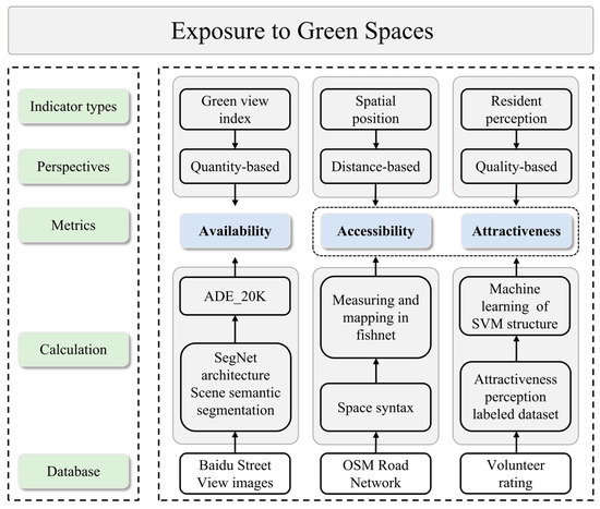
Figure 1.
GS exposure assessment framework.
- (1)
- Availability of GSs: This metric assesses the overall quantity of GSs, representing the source of GS exposure. We quantified the total amount of GSs from a visual perspective by collecting street view images and using semantic image segmentation techniques. This method facilitates a broad and precise measurement of GS exposure at an everyday-contact scale.
- (2)
- Accessibility of GSs: This metric signifies the ease with which one can reach GSs. This affects the likelihood and frequency of individuals encountering GSs, subsequently influencing GS exposure. To align with street view image data, we used spatial syntax to compute the accessibility of urban roads, thereby characterizing the accessibility of GSs.
- (3)
- Attractiveness of GSs: Attractiveness is a human-scale, subjective perceptual metric that, to some extent, represents the quality of GSs. The attractiveness of a GS can affect the visitation intent and duration of residents, further influencing GS exposure. Based on subjective attractiveness scores from street view images, we employed a machine learning model based on a support vector machine (SVM) to predict the city-scale attractiveness of GSs.
Using downtown Shanghai as a case study, we further applied the constructed GS exposure assessment framework to actual measurements. This study unveiled the influential role of the urban built environment in GS exposure from both micro and macro perspectives.
2.2. Study Area
Shanghai is situated between the 120°51′ E–122°12′ E longitudes and the 30°40′ N–31°53′ N latitudes. It is categorized as a megacity with a high density and is renowned for its historical and cultural significance. The city wields substantial international influence in sectors such as economics, finance, trade, and shipping. Covering a total area of 6340.5 km2, Shanghai comprises 16 administrative districts. Climatically, Shanghai has a subtropical monsoon climate with an annual average temperature of 25.8 °C. In terms of population, as of 2022, the city had a permanent residency of approximately 24.7589 million people. For this study, the chosen study area is downtown Shanghai (Figure 2), specifically the area inside the city’s outer ring. This includes Huangpu, Xuhui, Changning, Jing’an, Putuo, Hongkou, and Yangpu districts, as well as portions of Pudong New Area, Minhang, Baoshan, and Jiading districts, covering an area of 660 km2. This region boasts the longest developmental history in Shanghai, the highest level of urbanization, and the highest population density, making it particularly representative of the city as a whole. In recent years, with a shift in Shanghai’s urban planning policies from expansion-focused development to optimizing existing structures, emphasis has been placed on curbing haphazard urban construction, refining the city’s structure, and enhancing the quality of living environments. Consequently, measuring the exposure to GSs in downtown Shanghai is of paramount importance for guiding the city’s future developmental strategies.
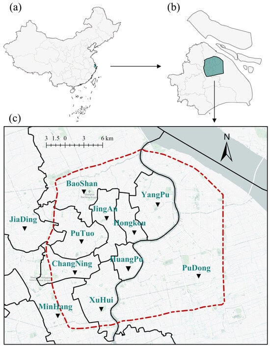
Figure 2.
Study area: (a) China, (b) Shanghai, (c) downtown Shanghai with the districts.
2.3. Street View Data Collection
This study collected street view images from downtown Shanghai for subsequent urban GS exposure measurements. The platform that was used for image collection was Baidu Maps (https://map.baidu.com, accessed on 23 August 2023) Using the Python language, we constructed HTTP_URLs and set up image capture points every 50 m on road networks, downloaded from OpenStreetMap (OSM), resulting in a total of 71,533 sampling points. With the help of a GIS, we calculated the viewing direction for each sampling point to ensure that all street view images were aligned with the forward direction of the road, thus ensuring the accuracy of the results. By developing a program in Python, we accessed Baidu Street View Map’s API to collect images with a pixel resolution of 600 × 480 from four different directions for each sampling point. After data cleaning and removing invalid data, we obtained 250,776 valid street view images, which were combined to produce a total of 62,694 panoramic street view images. The street view data collection was completed on 23 August 2023. The street view image collection process is illustrated in Figure 3.
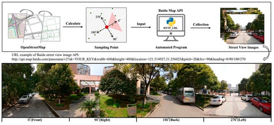
Figure 3.
Baidu street view image collection process.
2.4. Measurement of GSs’ Availability Based on Image Segmentation
Utilizing street view images combined with machine learning to identify the characteristics of urban built environments has been established as an effective research method [65,66]. In this study, we employed semantic image segmentation techniques using the convolutional neural network (CNN) structure to identify the proportional representation of visual elements in street view images. Among the numerous algorithms that have been developed for semantic segmentation, SegNet stands out due to its efficiency and effectiveness across various applications [67]. In our study, we used the SegNet algorithm, which is based on an encoder–decoder architecture, to semantically segment the street view images. This algorithm comprises two main components: an encoder and a decoder. The encoder is responsible for extracting and compressing the semantic information of objects from images, while the decoder restores this compressed information to the original image dimensions, achieving pixel-level classifications. A detailed representation of SegNet’s complete architecture and workflow is provided in Figure 4. We trained the semantic segmentation model using the ADE_20K dataset. This dataset can identify 150 types of urban environmental elements, such as sky, roads, cars, and trees, and has been proven to have a high accuracy [68]. The training results show an accuracy of 90.83% in the training set and 89.95% in the validation set, indicating that the model can effectively perform interpretive work on street view images segmentation. Subsequently, we summed up all the elements that could characterize urban GSs (including trees, grass, and plants) to obtain the measurement results for the availability of GSs. Additionally, based on previous research [69], we also extracted the segmentation results for other elements such as buildings, sky, and road to represent the characteristics of the urban built environment on a microscale.
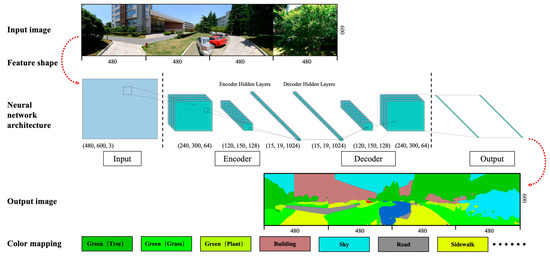
Figure 4.
Image segmentation process of street view images.
2.5. Measurement of GSs’ Accessibility Based on Spatial Syntax
Space syntax is a common method for measuring accessibility. It can abstract complex urban space situations into mathematical graphs and nodes. It uses mathematical topological relationships to describe the quantitative relationships between spaces, thereby exploring the impact of urban spatial forms on human spatial behavior. Due to the detailed nature of road data, they may interfere with the calculation of accessibility. Studies have shown that spatial syntax can enhance the understanding of urban layouts, and it is widely adopted in urban spatial analyses [70]. In this study, we used spatial syntax to calculate urban GSs’ accessibility. We used road network data from OSM as the original data. However, because of the detailed nature of the road data, they might interfere with accessibility calculations. To address this, we first incorporated a buffer for the roads using a GIS. We then extracted the central lines of these buffer zones, establishing a new road network. Finally, the network underwent street consolidation, street simplification, and topological treatments to ensure that it provided high-quality data for accessibility calculations. The calculation formula for spatial syntax is expressed in Equation (1):
where represents the accessibility value of space , denotes the shortest path from space to space , and represents the shortest path between space and that includes space ( < , = 1, 2, 3, …, n − 1, = 2, 3, 4, …, n).
Drawing from a prior study [71], we used a standard daily travel distance of 500 m for residents as the accessibility radius and calculated the accessibility value for each street. The computations and visualizations were conducted in depthmapX 0.8.0 [72].
2.6. Measurement of GSs’ Attractiveness Based on Machine Learning
Machine-learning-based predictions of urban environmental perceptions are widely employed in urban spatial quality measurements. These are characterized by their broad scope, high precision, and user-friendly operations. Such approaches provide precise data support for urban planners and administrators [73,74]. Based on this premise, our study employed a subjective perception prediction approach to assess the attractiveness of urban GSs. Following the experimental procedures of previous research [75,76], we recruited 32 volunteers to assess the attractiveness of street view images: 17 females and 15 males, with an average age of approximately 35 years and a local/nonlocal ratio of 1:1. We proved that this number of volunteers led to scientific and reliable data, and the accuracy of machine learning training conducted on this basis meets scientific requirements [77,78]. Each volunteer was assigned 50 streetscape images and was required to observe each image for no less than 30 s. The sampling method was not completely random. Volunteers were instructed to rate the attractiveness of the streetscape images, with a score of 1 indicating very unattractive, 2 somewhat unattractive, 3 neutral, 4 somewhat attractive, and 5 very attractive. Notably, all the volunteers’ scoring processes were conducted on Tencent Cloud servers.
Subsequently, we developed a prediction model based on the SVM to evaluate the attractiveness of GSs within the city. This model demonstrated exceptional performance in previous studies [79,80]. The training dataset is derived from the volunteers’ scores for the attractiveness of GSs, representing a quantification of human evaluations. Each score is associated with a corresponding GS image, which is preprocessed through image segmentation techniques to extract key image features as input variables. An SVM can help us score all street view images against a uniform standard, thereby facilitating the prediction of the attractiveness of urban GSs. To achieve a more precise model fit, we utilized the radial basis function as the kernel function. The mathematical expression for this SVM model is presented in Equation (2):
where represents the normal vector of the decision boundary. We aimed to minimize this objective function while adhering to the constraints that are described in Equation (3).
where represents the sample’s class label, denotes the sample’s feature vector, and b is the bias term.
During this process, we fine-tuned the SVM’s hyperparameters to enhance the model’s performance, thus completing the model’s training. We used 75% of the perceived attractiveness data to train the SVM model, with the remaining 25% serving as the validation set to test the model’s accuracy. Figure 5 illustrates the process of predicting the attractiveness of GSs.
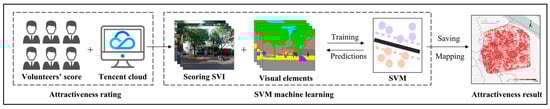
Figure 5.
Attractiveness prediction process based on SVM machine learning model.
2.7. Measurement of GS Exposure
In geographical research, data are often processed in the form of a fishnet (i.e., a fishnet grid), which facilitates the overlay of data at different scales [47]. In this study, the metrics of GS exposure were all mapped onto a 500 m × 500 m fishnet grid for subsequent calculations. The size of the fishnet was chosen based on the average daily travel distance of residents in the city, a criterion that has been validated in related studies [71]. The measurements for accessibility and attractiveness were normalized to better reflect the actual GS exposure. The specific calculation is expressed in Equation (4).
where Gi represents the GS exposure at location i, Qi denotes the visual proportion of GS at location i, Ci is the accessibility at location i, Ti is the attractiveness score at location i, and S represents the standard deviation.
Subsequently, we utilized principal component analysis (PCA) to further clarify the contributions of each GS exposure indicator. The varimax rotation method was applied to enhance interpretability. The calculation formula for PCA is expressed in Equation (5):
where Y represents the dimensionality-reduced data matrix, denotes the centered data matrix, and Pk is the matrix composed of the selected k eigenvectors.
To further quantify the spatial distribution characteristics of GS exposure in downtown Shanghai, we constructed 13 concentric circles, with the geometric center of the study area as the center point and intervals of 1.5 km. The innermost circle had a radius of 1.5 km, and each subsequent circle increased by 1.5 km, forming 13 urban belts. These urban belts covered the majority of the study area.
2.8. Analysis of the Association between GS Exposure and the Built Environment
2.8.1. Measurement of Micro and Macro Characteristics of Built Environment
This study measured the built environment characteristics at both the micro- and macroscales. The microscale built environment typically refers to the built environment features that humans can directly perceive. Therefore, the built environment features that were used in this study were extracted from the street-scale streetscape image scene elements of the segmentation results. We extracted the four most dominant features that were not related to GSs: building, sky, roadway, and sidewalk. These four elements are strong representations of built environment characteristics and are frequently used in related studies [63,66,81]. To match the data on GS exposure, we mapped the built environment data onto a grid corresponding to the GS exposure, with the value in each grid being the average of the sampled data points.
Measuring macroscale built environment characteristics is based on the 5Ds framework [82,83]. The 5Ds framework evaluates urban built characteristics from a functional perspective and is widely used in urban studies [84,85]. It includes the density, design, diversity, destination accessibility, and distance to transit of urban built environment features. Following a previous study [69], the density is measured by the building density in each grid. Design is evaluated by means of the road network density and the number of intersections within the grid. Further, we utilized points of interest (POIs) data to measure other metrics. POI data provide comprehensive and accurate information on urban land use. The POI dataset for this study was retrieved using the API provided by Gaode Map (https://lbs.amap.com/, accessed on 26 June 2023). POIs in the Gaode Map database are divided into over 20 categories. We reclassified the original POI dataset into five categories representing essential urban functions: residential, enterprises, commercial, public services, and entertainment. After removing duplicates and irrelevant data, we obtained a total of 861,028 valid POI entries. The descriptive statistics of these five categories of POIs are presented in Table 1. The diversity was calculated based on the entropy score of these POI data in each grid [86], expressed as Equation (6):
where M represents POIs diversity, pi denotes the proportion of the I type of POI, and n is the total number of POI types that are presented in the grid. The destination accessibility is measured by the total number of the five types of POIs in each grid. The distance to transit is gauged by the number of transportation hubs, including bus stations, subway stations, car parks, train stations, etc. The statistical features of each built environment factor are shown in Table 2.

Table 1.
The five fundamental POI types and the corresponding categories in the original Gaode Map.
Table 2.
Summary statistics for all variables in downtown Shanghai.
2.8.2. Regression Analysis
This study conducted a regression analysis of the GS exposure in downtown Shanghai and its urban built environment to further elucidate their association. Three distinct regression models were employed, including the ordinary least squares (OLS) regression model, the spatial lag model (SLM), and the spatial error model (SEM).
The OLS linear regression model is a global model that estimates the parameters of the explanatory variables in a linear model by minimizing the sum of squared differences between the predicted and observed values in a dataset. The fundamental assumptions of the OLS model are that the residuals are random and homoscedastic [87]. Its formula is expressed in Equation (7):
where Y is the dependent variable, X is the matrix of explanatory variables, β is the vector of coefficients, and ϵ is the vector of random error terms.
However, it should be noted that OLS models may exhibit biases in analyses involving spatial data. Such biases often arise due to spatial dependencies, wherein the value that is observed at one location is influenced by values at neighboring locations. To address this issue, the present study employs both the SLM and the SEM. The SLM postulates that spatial dependencies may stem from the autocorrelation of the dependent variable [69]. The computational formula for the SLM is expressed in Equation (8):
where ρ is the coefficient of spatial autocorrelation, wij is the spatial weight between geographic units i and j, and the other symbols are the same as in the OLS model.
The SEM tends to consider the autocorrelation of the error terms [69]. Its calculation formula is expressed in Equation (9):
where λ is the coefficient for the spatial error autocorrelation, wij is the spatial weight between geographic units i and j, and the other symbols are the same as in the OLS model.
In the statistical analysis, we used the cells of a fishnet (i.e., grid cells) as the basic spatial units and generated spatial weights using queen contiguity. The spatial regression models were run in GeoDa 1.20.0.36 [88].
2.8.3. Geodetector Analysis
Geodetector is a spatial analysis method used to detect spatial heterogeneity and reveal its underlying driving forces [89]. It is widely applied in the research of geography, ecology, sociology, and related fields [90,91]. The foundational principle of Geodetector is that it partitions the total sample into multiple subsamples and evaluates the spatial heterogeneity and variable relationships by means of variance. If the sum of variances of the subsamples is smaller than the total variance of all samples, spatial differences exist. If the spatial distributions of two variables tend to be consistent, a statistical correlation exists between them [92]. Pertinent to this study, if the spatial variation in GS exposure is triggered by a specific factor, then the spatial distribution of this factor should share similarities with that of the GS exposure. The Geodetector method utilizes the power of the determinant () to reflect the spatial correlation between factors X and Y and to identify the driving effect of the factor on the dependent variable. Its calculation formula is expressed in Equation (10):
where denotes the explanatory power of a factor on the variation in GS exposure; represents the number of samples in the study area; is the number of samples in region (category) of factor X; is the total variance of Y in the study area; is the variance of Y in region of factor X; and L denotes the number of regions (categories) for factor X. A higher value of implies that X has a greater explanatory power on Y, and vice versa.
Geodetector discerns the interactive effects between different factors Xs, assessing whether the joint effect of factors X1 and X2 either amplifies or attenuates the explanatory power on the dependent variable Y, or if their impacts on Y are mutually independent [93]. This method of assessment calculates the values of two factors of Y, and . The next step is to compute the interactive q value, denoted as , which is formed by the tangent of the superimposed variables and . This value is then compared to and to indicate the type of interaction between the two variables. Specifically, if < min(, it indicates nonlinear attenuation. If min( < < max(, it denotes single-factor nonlinear attenuation. If > max(, it signifies dual-factor enhancement. If = + , it points to dual-factor independence. And if > + , it indicates nonlinear enhancement.
3. Results
3.1. Measurement of GS Exposure Metrics
The GS exposure metrics were visualized on a map using a grid-like representation, enabling better observation of their spatial distribution. Figure 6 depicts the distribution pattern of the availability of GSs as “low in the center, high around the edges”. This pattern might be attributed to the high construction density in central urban areas. A high construction density usually equates to fewer available green areas. The mean value of availability was 0.242, with a standard deviation of 0.092. In most regions, the availability was clustered around the mean, generally tending to be on the lower side. The spatial distribution of the accessibility of GSs demonstrated a “low–high–low” pattern from the city center outward. This might have stemmed from the evolution of urban development and road construction scenarios. Due to traffic congestion and land use restrictions, the accessibility of GSs in the central region was relatively low. However, in the transitional zone between the center and the periphery, the accessibility of GSs was relatively high, likely due to better road infrastructure and traffic conditions. The mean value of accessibility was 0.349, with a standard deviation of 0.145, indicating variations in attractiveness across different regions. The spatial distribution of the attractiveness of GSs resembled that of accessibility, but the southwestern region exhibited higher attractiveness. This might be due to the superior landscape quality and a higher number of recreational facilities in that area. The mean value for attractiveness was 0.492, with a standard deviation of 0.177. This suggested that while attractiveness was generally high in most regions, there were some fluctuations. The Gaussian fitting results indicated that all three indices followed a normal distribution.
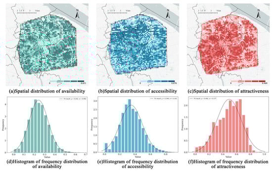
Figure 6.
Spatial distribution and histogram of frequency distribution of three GS exposure metrics.
3.2. GS Exposure Measurements and Spatial Distribution Characteristics
The results for GS exposure were normalized and are presented in a grid pattern in Figure 7. Downtown Shanghai displayed a “low–high–low” trend in GS exposure from the center to the outskirts, with a low overall exposure average value of 0.177. Areas of minimal exposure were primarily found in the convergence of Jing’an, Hongkou, and Huangpu districts and the periphery of the city center. Both high and low levels of urbanization seemed to be detrimental to GS exposure. Based on the city’s developmental pattern, central locations with older, denser developments restricted GS allocation. Conversely, the outer city center, which was still developing at the time, lacked a well-developed infrastructure. Representative images showed that central areas were densely populated with mixed elements, but adding greenery could significantly enhance GS exposure. Peripheral areas, mostly consisting of highways or elevated roads, offered expansive views. Despite having high-quality GSs, the exposure remained low due to their geographic location and accessibility constraints. Numbers 1–8 represent the street view image display of typical areas.
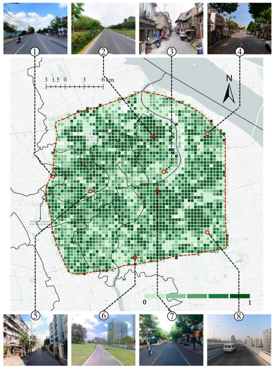
Figure 7.
Spatial distribution of GS exposure.
The analysis of urban belts can better assist us in understanding the spatial structure of GS exposure. As depicted in Figure 8a, we aggregated and averaged the GS exposure values within these urban belts, revealing exposure variation across the city. Figure 8b compares the average exposure values for each urban belt, showing a range from 0.132 to 0.232. Using the distance from the inner city as the independent variable and the GS exposure average as the dependent variable, we performed a quadratic fit, with results presented in Figure 8c. The quadratic term coefficient was −0.002, the linear coefficient was 0.025, and the constant was 0.135. This suggested a pronounced trend of GS exposure increasing when moving from the inner city to the outskirts and then decreasing again, highlighting the spatial inequality of GS exposure.

Figure 8.
Mapping of GS exposure changes using concentric circles from downtown Shanghai.
By conducting a PCA on three pivotal metrics of urban GS exposure, we found that the first principal component (PC1) explained 53.4% of the total variance (Table 3). This indicates that PC1 likely encapsulated shared traits among the three metrics, serving as a comprehensive GS exposure measure. PC1 and PC2 accounted for almost 87% of the total variance, emphasizing their significance in characterizing GS exposure. In Table 4, we observed that each indicator is independently explained by different principal components. The results indicate that attractiveness is closely related to PC1, suggesting that attractiveness plays a major role in assessing exposure to green spaces. Accessibility is entirely correlated with PC2, indicating that accessibility is the second most significant factor. Availability is fully explained by PC3, and although it contributes the least to the total variance, it remains a decisive factor in determining whether residents can actually use GSs. This further highlights the leading role of the quality of GSs focused on in this study in the GS exposure. In practical urban planning and construction, the accessibility and attractiveness of GSs need to be given priority to effectively enhance urban environmental quality.
Table 3.
Explained variance ratio in principal component analysis.
Table 4.
Principal component loadings for green space exposure metrics.
3.3. Regression Analysis Results
We assessed the multicollinearity among the independent variables using the variance inflation factor (VIF). The results showed that all VIF values of the variables were below 4, indicating no multicollinearity issues, which ensured that the statistical results were reliable. The Lagrange multiplier (LM) and robust LM tests are often employed to identify the suitability of spatial models. This study employed the LM test to determine which model is more suitable (Table 5). The Koenker–Bassett test was highly significant, suggesting spatial heterogeneity among the built environment variables, thus necessitating further spatial regression analysis using the SLM and SEM. Our results revealed that both the micro- and macrolevel SLM models had higher values of the LM and robust LM. Thus, this study primarily focused on the regression results of the SLM.
Table 5.
Model setting verification of micro- and macroscale built environment.
The results of the regression model of GS exposure reveal the significant impact of built environment factors on GS exposure (Table 6). The microscale and macroscale, respectively, represent the human perspective and the urban perspective, which can help us gain a more comprehensive understanding of the urban built environment. The results indicated that the SLM outperformed the SEM and OLS model in terms of R2, AIC, and LLV, suggesting that the SLM model was more capable of explaining the association between urban built environment factors and GS exposure. At the microscale of the built environment, both the building and sky view indexes are significantly negatively correlated with GS exposure (p < 0.001), with coefficients of −0.373 and −0.498, respectively. The sidewalk view index is significantly positively correlated with GS exposure (p < 0.01), with a coefficient of 0.263. This indicates that an increase in the building and sky view indexes, or a decrease in the sidewalk view index, will lead to a reduction in GS exposure. The roadway view index did not show a significant relationship with GS exposure in any model (p > 0.05). At the macroscale, the building density is positively correlated with GS exposure (p < 0.001), as is the POI diversity (p < 0.01). The number of POIs is negatively correlated with GS exposure (p < 0.05). Street intersections, street density, and transit stops do not show a significant relationship with GS exposure (p > 0.05). Overall, both the micro- and macroscale factors of the built environment significantly affect GS exposure, but the microscale built environment factors have a stronger explanatory power.
Table 6.
Results of regression models of GS exposure in fishnet grid.
3.4. Geodetector Analysis Results
In this study, Geodetector was employed to further delve into the relationship between built environment factors and GS exposure. Figure 9a depicts the magnitude of the influence that was exerted by different built environment factors on GS exposure. The findings revealed that the sky view index had the highest q-statistic, 0.102, with a significant p-value below 0.001, suggesting its paramount influence on GS exposure. Both the POI quantity and the sidewalk view index also demonstrated certain levels of influence, with q-statistics of 0.040 and 0.037, respectively, and both with p-values below 0.001. While other factors, such as the building view index, building density, and diversity of POIs, had relatively lower q-statistics, they remained statistically significant due to their p-values being below 0.001. Notably, both the roadway view index and street intersections exhibited negligible effects on GS exposure, which was consistent with the results from the structural equation model regression.
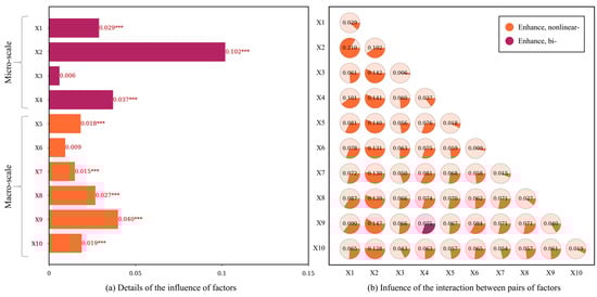
Figure 9.
Geodetector analysis results of GS exposure and built environment. *** denotes significance at the 0.1% level.
When exploring how built environment factors affect GS exposure, singular factors can rarely explain the GS exposure independently, and interactions among factors should be considered. Previous studies on interactions relied primarily on the product of factors. However, in real urban settings, these interactions are intricate and cannot be fully explained by merely multiplying factors. Geodetector is capable of identifying the magnitude and interrelationships of interactions between pairs of factors. As depicted in Figure 9b, the sky view index’s interaction effects with other factors often have higher values, such as its interaction coefficient with the building view index of 0.210, highlighting its role as a key factor in multifactorial interactions. Additionally, the POI quantity also displayed considerable interaction effects with other factors, such as its interaction with street intersections of 0.084, suggesting its significant role in complex urban environments. In contrast, the roadway view index and street intersections had relatively low interaction effects with other factors, echoing the earlier single-factor analysis, which further confirmed their minimal impact on GS exposure. Intriguingly, nearly all the interactions exhibited nonlinear enhancement, implying that the relationships among these factors are complex and nonlinear, and GS exposure cannot be simply predicted by cumulating the impacts of individual factors. The only exception was the interaction between the POI quantity and the sidewalk view index, possibly indicating that their combined effect on the GS exposure was linear or nearly linear. These findings shed light on the interaction effects between built environment factors, suggesting that they operate within a complex milieu of multiple interacting elements, which in turn influence the GSs.
4. Discussion
4.1. Multidimensional Framework for Measuring Urban GS Exposure
Although the significance of urban GSs is universally recognized, neglecting issues such as their accessibility to residents, their ease of use, and residents’ daily interactions with these spaces can lead to disparities between GS construction and utilization. This results in actual imbalances in their distribution. Hence, devising a comprehensive, scientific, and practical framework for measuring GS exposure is of paramount importance. The combination of street view images and machine learning can help us revisit GSs from the perspective of streets or at even smaller scales, integrating previously hard-to-obtain perceptual data into the research on GSs [63,94]. This approach allows for a more comprehensive and accurate discussion of the efficacy of GSs, moving beyond simply measuring their quantity. GS exposure is a human-centric evaluation indicator, and this framework is conducted from a human-centric perspective, specifically reflected in three aspects: (1) The research data are derived from street view images. These are façade images that are shot from a human viewpoint, providing a method for observing the urban environment from a human-centric perspective, laying the foundation for this study. (2) The assessment framework that is constructed in this study incorporates subjective human perception. Residents’ perception of the attractiveness of GSs is an important indicator of this framework, helping us to examine GSs from the residents’ perspective. (3) This study focuses on the street scale, assessing the GS exposure that is most relevant to residents’ daily lives, revealing the impact of daily GS exposure, and assisting in enhancing the social welfare effect of urban GSs.
More importantly, our proposed GS exposure measurement framework has scalability and application potential. Acquiring high-resolution remote sensing images often requires approval from governments or relevant agencies. In contrast, high-precision street view images are entirely open-source and much easier to acquire than high-resolution remote sensing images, and they can also support the measurement of GS exposure. With the support of this open-source street view big data, the GS exposure measurement that we developed in this study can be conveniently transferred for use in different urban spaces and widely applied in future urban planning and policy making.
4.2. Spatial Variation in GS Exposure in Downtown Shanghai
This study delved into the GS exposure in downtown Shanghai, revealing a strong correlation between GS exposure and urban spaces. The study found spatial differences in the availability, accessibility, and attractiveness of GSs, which were closely tied to factors such as the urban construction density, transportation conditions, and landscape quality. Our measurement results indicated a “low–high–low” spatial distribution pattern for GS exposure, which was directly related to the city’s developmental pattern and construction density. Central areas exhibited lower GS exposure, possibly due to their high construction density and land use restrictions. As they are typically hubs for commerce, culture, and politics with high land prices, the allocation of GSs in these regions is often constrained. This phenomenon is observed in many major cities, reflecting the contradiction between commercial and residential space demands and GS provisions [95,96]. In contrast to the city center, while peripheral urban regions might offer more room for GS development, the GS exposure remained low in peripheral urban regions due to inadequate infrastructure and geographical constraints. This suggests that, during the initial phases of urban development, the planning and construction of GSs are often overlooked, potentially impacting a city’s sustainable growth and its residents’ quality of life. Transition areas between the city center and the outskirts, with better road construction and transportation conditions, exhibit higher GS accessibility [97]. The elevated GS exposure levels in these regions can be attributed to their unique position during urban development phases. Being focal areas of urban expansion with superior infrastructure and public services, GS planning and construction are often focused on more here [98].
Considering the population distribution of Shanghai, the differences in GS exposure directly impact the equity of residents’ wellbeing. The population distribution in Shanghai is characterized by a dense center and sparsely populated outskirts [99], which directly interact with the “low–high–low” distribution pattern of GSs. This means that a large population in the central area has limited exposure to GSs. Moreover, the central area comprises many old neighborhoods, which are predominantly inhabited by elderly people [100] who have limited mobility. The negative effects of a low GS exposure are more pronounced in these living areas. With the trend of an ageing population, this issue warrants significant attention. Our study also found that in the central urban areas of Shanghai, the exposure to GSs was not clearly associated with residential areas. This suggests that the construction of GSs at the street scale has been somewhat neglected in past residential area developments. This also adversely affects the wellbeing of urban residents.
4.3. Micro and Macro Influences of Built Environment on GS Exposure
This study, at both the micro- and macroscales, extracted features of the urban built environment and conducted a cross-sectional analysis of GS exposure in relation to these features, aiming to uncover how urban construction influences GS exposure. Utilizing structural equation modeling, we regressed urban built environment factors at both scales. At the microlevel, we identified that the building and sky view indexes had significant negative correlations with GS exposure, while the sidewalk view index was positively correlated. An increased building view index typically signified building clusters encroaching upon GSs. Areas with a high sky view index often had lesser-developed infrastructures, leading to limited greenery. Well-constructed sidewalks increased the accessibility of GSs and the likelihood of residents visiting them, consequently enhancing GS exposure, which is consistent with a prior study [101]. By optimizing urban spatial layouts and improving the combination of sidewalks and GSs, GS exposure can be effectively enhanced [102].
At the macroscale, the building density was positively correlated with GS exposure. Although many studies have demonstrated that a high building density negatively affects the quantity and density of GSs [96], this is not necessarily the case for GS exposure. GS exposure needs to be considered comprehensively, taking into account the availability, accessibility, and attractiveness of GSs. In underdeveloped urban areas with a very low building density, there may be abundant greenery, but the area’s accessibility is poor, which discourages residents from entering, and the quality of the GS is not guaranteed. Paul and Bardhan argue that for areas lacking blue and GSs, increasing building sites is an effective improvement strategy [103], which supports the results of this study. This outcome also illustrates that, for cities, both excessive development and a lack of construction are detrimental to enhancing GS exposure.
A diverse range of POIs fostered GS exposure, while an excessive number of POIs could lead to spatial congestion and organizational chaos, emphasizing the importance of quality over quantity in urban planning. This underscored the importance of maintaining diverse POIs, avoiding overconcentration of similar types [104,105], and thereby sustaining adequate GS exposure. Geographical detector analysis further revealed the interactive effects among built environment factors, indicating their operation within a complex, multifactorial context that affects GS exposure. These findings provide a more comprehensive understanding of the relationship between the urban built environment and GS exposure, offering strong theoretical support for future urban planning and resource management.
In conclusion, through empirical analysis of downtown Shanghai, this study highlights the significant impact of the urban built environment on GS exposure, offering scientific backing for urban planners and managers and aiming to provide a comprehensive and in-depth theoretical foundation and practical guidance for sustainable urban development.
4.4. Policy Suggestions
China has fully transitioned from incremental development to stock development, and this is particularly true for Shanghai, a megacity in China. Optimizing the spatial structure and improving the quality of landscapes directly affect Shanghai’s urban vitality and residents’ wellbeing and are central to the city’s future urban planning and GS construction. The “Shanghai Municipal Land Space Planning (2020–2040)” framework, released by the Shanghai Municipal Government, clearly proposes to optimize the layout of urban GSs and enhance urban ecological functions, providing policy support for this study.
The findings of this study have important implications for urban planning. Firstly, urban planners need to re-examine the configuration of GSs in central urban areas and explore how to improve GS exposure under conditions of a high construction density. We suggest exploring innovative greening methods, such as rooftop greening and vertical greening, to make full use of limited spaces. Additionally, through urban renewal projects, transforming abandoned industrial lands into public GSs can bring more GSs to urban centers. Secondly, for the outskirts and newly developed areas, GS planning and construction should be thought through in the early stages of urban planning to ensure a sufficient proportion of public green lands and ecological lands, promoting sustainable urban development. Lastly, given the characteristics of higher GS exposure in transitional areas, it is important to strengthen the connectivity and accessibility of GSs in these areas by setting up more pedestrian paths and bike lanes, among other infrastructures, to increase residents’ utilization of and satisfaction with GSs. This will help improve the quality of life for urban residents and the overall environmental quality of the city.
In summary, there is a significant correlation between the results of GS exposure measurements and urban development patterns, providing valuable references for urban planning and management. By optimizing the configuration of GSs and enhancing their accessibility and attractiveness, we can promote the green development of cities, creating more livable and sustainable urban environments.
4.5. Limitations and Future Directions
We constructed a GS exposure assessment framework based on machine learning and street view imagery. Subsequently, we extracted urban built environment factors at both the micro- and macroscales, revealing the impact of the urban built environment on GS exposure. Our study results deepen our understanding of GS measurement and facilitate the practical application of our findings in urban construction. However, our study has its limitations, which will require further exploration and improvement in future research.
Firstly, we established our GS exposure assessment framework by selecting three dimensions: availability, accessibility, and attractiveness. Nevertheless, there are other aspects of the pathways through which GSs function. For instance, Gascon et al. suggested that the benefits of GSs to human health are achieved through “mediators”, such as improved air quality or noise reduction [106]. These comprehensive factors should be incorporated into future assessment frameworks to achieve a holistic understanding of the role of GSs.
Secondly, our study utilized a cross-sectional analysis to examine the influence of urban built environment factors on GS exposure, lacking a consideration for time series. Xing et al. pointed out that a comprehensive understanding of the spatial and temporal dynamics of GSs is crucial for planners and decision makers [107]. Future research should encompass broader spatial and temporal dimensions, incorporating socioeconomic factors and policy environments, to fully understand the relationship between urban development and GS exposure.
Lastly, it is essential to recognize that the goal of GS exposure is to enhance human wellbeing. Future studies should integrate population data or human mobility patterns to promote precise measurements at the resident level. Furthermore, incorporating public health data will shed light on the intricate mechanisms through which GS exposure impacts residents’ health.
5. Conclusions
In the context of rapid urbanization, evaluating GS exposure is crucial for enhancing urban quality and residents’ wellbeing. This study addressed the limitations of previous evaluation methods by employing machine learning and street view images to construct a novel, human-centric framework for assessing GS exposure. It comprehensively examined the efficacy of GSs regarding the aspects of availability, accessibility, and attractiveness. Supported by open-source street view big data, this framework boasts considerable scalability and operability, allowing for its application across different cities and holding the potential to impact urban planning, city management, and public health.
Using downtown Shanghai as a case study, we demonstrate the practicality of this evaluation framework. This study found that the spatial distribution of GS exposure in downtown Shanghai exhibits a clearly layered structure, increasing and then decreasing from the center to the outskirts. This reflects significant spatial heterogeneity in GS exposure, which becomes evident with urban development. Thanks to the establishment of this assessment framework, we further reveal the complex relationship between GS exposure and the urban built environment on both the micro- and macroscales. On a microscale, the building and sky view indexes are significantly negatively correlated with GS exposure, while the sidewalk view index is positively correlated, indicating that both the excessive clustering and dispersion of buildings are detrimental to GS construction, and that well-developed pedestrian pathways can enhance residents’ exposure to GSs. On a macroscale, the building density is positively correlated with GS exposure, showing that areas with higher urban development levels have greater GS exposure. Additionally, a diverse range of POIs can promote GS exposure, while an excessive number may have the opposite effect.
Overall, this study provides an efficient and scientific tool with which urban researchers and managers can assess and improve urban GS exposure. By thoroughly analyzing the case of downtown Shanghai, this study not only reveals the spatial distribution patterns and influencing factors of GS exposure but also offers valuable experiences and methods for other cities. This contributes to promoting sustainable urban development, enhancing the wellbeing of city residents and providing scientific guidance for urban planning and policymaking.
Author Contributions
Conceptualization, T.Z. and Y.H.; data curation, Y.L.; funding acquisition, Y.H.; methodology, T.Z. and L.W.; supervision, Y.H.; visualization, T.Z. and W.Z.; writing—original draft, T.Z., L.W. and Y.H.; writing—review and editing, T.Z., L.W. and Y.H. All authors have read and agreed to the published version of the manuscript.
Funding
This research was funded by Reconstructing the Architecture System based on the Coherence Mechanism of “Architecture-human-environment” in the Chinese Context, Key Project of National Natural Science Foundation of China, grant number 52038007.
Data Availability Statement
The data presented in this study are available on request from the corresponding author. In order to promote future research and the dissemination of this innovation, the source data and code for this research can be found at https://github.com/Ericzzz66/ZTLUrbanStudies/tree/main/Changlifang_GSexposureframework (accessed on 29 March 2024).
Conflicts of Interest
The authors declare no conflicts of interest.
Correction Statement
This article has been republished with a minor correction to the existing affiliation information. This change does not affect the scientific content of the article.
References
- Onishi, A.; Cao, X.; Ito, T.; Shi, F.; Imura, H. Evaluating the Potential for Urban Heat-Island Mitigation by Greening Parking Lots. Urban For. Urban Green. 2010, 9, 323–332. [Google Scholar] [CrossRef]
- Liu, W.; Chen, W.; Peng, C. Assessing the Effectiveness of Green Infrastructures on Urban Flooding Reduction: A Community Scale Study. Ecol. Model. 2014, 291, 6–14. [Google Scholar] [CrossRef]
- Yang, J.; Guan, Y.; Xia, J.C.; Jin, C.; Li, X. Spatiotemporal Variation Characteristics of Green Space Ecosystem Service Value at Urban Fringes: A Case Study on Ganjingzi District in Dalian, China. Sci. Total Environ. 2018, 639, 1453–1461. [Google Scholar] [CrossRef] [PubMed]
- Jaafari, S.; Shabani, A.A.; Moeinaddini, M.; Danehkar, A.; Sakieh, Y. Applying Landscape Metrics and Structural Equation Modeling to Predict the Effect of Urban Green Space on Air Pollution and Respiratory Mortality in Tehran. Environ. Monit. Assess. 2020, 192, 412. [Google Scholar] [CrossRef] [PubMed]
- Recio, A.; Linares, C.; Banegas, J.R.; Díaz, J. Road Traffic Noise Effects on Cardiovascular, Respiratory, and Metabolic Health: An Integrative Model of Biological Mechanisms. Environ. Res. 2016, 146, 359–370. [Google Scholar] [CrossRef] [PubMed]
- Qin, B.; Zhu, W.; Wang, J.; Peng, Y. Understanding the Relationship between Neighbourhood Green Space and Mental Wellbeing: A Case Study of Beijing, China. Cities 2021, 109, 103039. [Google Scholar] [CrossRef]
- Wachsmuth, D.; Angelo, H. Green and Gray: New Ideologies of Nature in Urban Sustainability Policy. Ann. Am. Assoc. Geogr. 2018, 108, 1038–1056. [Google Scholar] [CrossRef]
- Bush, J. The Role of Local Government Greening Policies in the Transition towards Nature-Based Cities. Environ. Innov. Soc. Transit. 2020, 35, 35–44. [Google Scholar] [CrossRef]
- Kolimenakis, A.; Solomou, A.D.; Proutsos, N.; Avramidou, E.V.; Korakaki, E.; Karetsos, G.; Maroulis, G.; Papagiannis, E.; Tsagkari, K. The Socioeconomic Welfare of Urban Green Areas and Parks; A Literature Review of Available Evidence. Sustainability 2021, 13, 7863. [Google Scholar] [CrossRef]
- Bratman, G.N.; Anderson, C.B.; Berman, M.G.; Cochran, B.; De Vries, S.; Flanders, J.; Folke, C.; Frumkin, H.; Gross, J.J.; Hartig, T.; et al. Nature and Mental Health: An Ecosystem Service Perspective. Sci. Adv. 2019, 5, eaax0903. [Google Scholar] [CrossRef]
- Hartig, T.; Mitchell, R.; De Vries, S.; Frumkin, H. Nature and Health. Annu. Rev. Public Health 2014, 35, 207–228. [Google Scholar] [CrossRef]
- Van Den Berg, A.E.; Jorgensen, A.; Wilson, E.R. Evaluating Restoration in Urban Green Spaces: Does Setting Type Make a Difference? Landsc. Urban Plan. 2014, 127, 173–181. [Google Scholar] [CrossRef]
- Lu, Y. Using Google Street View to Investigate the Association between Street Greenery and Physical Activity. Landsc. Urban Plan. 2019, 191, 103435. [Google Scholar] [CrossRef]
- Tang, J.; Long, Y. Measuring Visual Quality of Street Space and Its Temporal Variation: Methodology and Its Application in the Hutong Area in Beijing. Landsc. Urban Plan. 2019, 191, 103436. [Google Scholar] [CrossRef]
- Berman, M.G.; Kross, E.; Krpan, K.M.; Askren, M.K.; Burson, A.; Deldin, P.J.; Kaplan, S.; Sherdell, L.; Gotlib, I.H.; Jonides, J. Interacting with Nature Improves Cognition and Affect for Individuals with Depression. J. Affect. Disord. 2012, 140, 300–305. [Google Scholar] [CrossRef]
- Wang, R.; Zhao, J.; Meitner, M.J.; Hu, Y.; Xu, X. Characteristics of Urban Green Spaces in Relation to Aesthetic Preference and Stress Recovery. Urban For. Urban Green. 2019, 41, 6–13. [Google Scholar] [CrossRef]
- Schertz, K.E.; Berman, M.G. Understanding Nature and Its Cognitive Benefits. Curr. Dir. Psychol. Sci. 2019, 28, 496–502. [Google Scholar] [CrossRef]
- Wang, R.; Xue, D.; Liu, Y.; Chen, H.; Qiu, Y. The Relationship between Urbanization and Depression in China: The Mediating Role of Neighborhood Social Capital. Int. J. Equity Health 2018, 17, 105. [Google Scholar] [CrossRef]
- Gong, F.-Y.; Zeng, Z.-C.; Zhang, F.; Li, X.; Ng, E.; Norford, L.K. Mapping Sky, Tree, and Building View Factors of Street Canyons in a High-Density Urban Environment. Build. Environ. 2018, 134, 155–167. [Google Scholar] [CrossRef]
- Ye, Y.; Richards, D.; Lu, Y.; Song, X.; Zhuang, Y.; Zeng, W.; Zhong, T. Measuring Daily Accessed Street Greenery: A Human-Scale Approach for Informing Better Urban Planning Practices. Landsc. Urban Plan. 2019, 191, 103434. [Google Scholar] [CrossRef]
- Williams, D.; Worster, D. The Wealth of Nature: Environmental History and the Ecological Imagination. J. Wildl. Manag. 1994, 58, 386. [Google Scholar] [CrossRef]
- Maas, J. Green Space, Urbanity, and Health: How Strong Is the Relation? J. Epidemiol. Community Health 2006, 60, 587–592. [Google Scholar] [CrossRef] [PubMed]
- Fuller, R.A.; Irvine, K.N.; Devine-Wright, P.; Warren, P.H.; Gaston, K.J. Psychological Benefits of Greenspace Increase with Biodiversity. Biol. Lett. 2007, 3, 390–394. [Google Scholar] [CrossRef] [PubMed]
- Maas, J.; Spreeuwenberg, P.; Van Winsum-Westra, M.; Verheij, R.A.; Vries, S.; Groenewegen, P.P. Is Green Space in the Living Environment Associated with People’s Feelings of Social Safety? Environ. Plan. Econ. Space 2009, 41, 1763–1777. [Google Scholar] [CrossRef]
- Qureshi, S.; Breuste, J.H.; Lindley, S.J. Green Space Functionality Along an Urban Gradient in Karachi, Pakistan: A Socio-Ecological Study. Hum. Ecol. 2010, 38, 283–294. [Google Scholar] [CrossRef]
- Home, R.; Bauer, N.; Hunziker, M. Cultural and Biological Determinants in the Evaluation of Urban Green Spaces. Environ. Behav. 2010, 42, 494–523. [Google Scholar] [CrossRef]
- Gong, Y.; Gallacher, J.; Palmer, S.; Fone, D. Neighbourhood Green Space, Physical Function and Participation in Physical Activities among Elderly Men: The Caerphilly Prospective Study. Int. J. Behav. Nutr. Phys. Act. 2014, 11, 40. [Google Scholar] [CrossRef] [PubMed]
- Zhang, R.; Zhang, C.-Q.; Rhodes, R.E. The Pathways Linking Objectively-Measured Greenspace Exposure and Mental Health: A Systematic Review of Observational Studies. Environ. Res. 2021, 198, 111233. [Google Scholar] [CrossRef] [PubMed]
- Paul, L.A.; Hystad, P.; Burnett, R.T.; Kwong, J.C.; Crouse, D.L.; Van Donkelaar, A.; Tu, K.; Lavigne, E.; Copes, R.; Martin, R.V.; et al. Urban Green Space and the Risks of Dementia and Stroke. Environ. Res. 2020, 186, 109520. [Google Scholar] [CrossRef]
- Russette, H.; Graham, J.; Holden, Z.; Semmens, E.O.; Williams, E.; Landguth, E.L. Greenspace Exposure and COVID-19 Mortality in the United States: January–July 2020. Environ. Res. 2021, 198, 111195. [Google Scholar] [CrossRef]
- Zhang, J.; Yu, Z.; Cheng, Y.; Sha, X.; Zhang, H. A Novel Hierarchical Framework to Evaluate Residential Exposure to Green Spaces. Landsc. Ecol. 2022, 37, 895–911. [Google Scholar] [CrossRef]
- Gascon, M.; Cirach, M.; Martínez, D.; Dadvand, P.; Valentín, A.; Plasència, A.; Nieuwenhuijsen, M.J. Normalized Difference Vegetation Index (NDVI) as a Marker of Surrounding Greenness in Epidemiological Studies: The Case of Barcelona City. Urban For. Urban Green. 2016, 19, 88–94. [Google Scholar] [CrossRef]
- Pinault, L.; Christidis, T.; Toyib, O.; Crouse, D.L. Statistics Canada Ethnocultural and Socioeconomic Disparities in Exposure to Residential Greenness within Urban Canada. Health Rep. 2021, 32, 3–14. [Google Scholar] [CrossRef]
- Zhang, J.; Liu, Y.; Zhou, S.; Cheng, Y.; Zhao, B. Do Various Dimensions of Exposure Metrics Affect Biopsychosocial Pathways Linking Green Spaces to Mental Health? A Cross-Sectional Study in Nanjing, China. Landsc. Urban Plan. 2022, 226, 104494. [Google Scholar] [CrossRef]
- Helbich, M. Spatiotemporal Contextual Uncertainties in Green Space Exposure Measures: Exploring a Time Series of the Normalized Difference Vegetation Indices. Int. J. Environ. Res. Public. Health 2019, 16, 852. [Google Scholar] [CrossRef]
- Berto, R. The Role of Nature in Coping with Psycho-Physiological Stress: A Literature Review on Restorativeness. Behav. Sci. 2014, 4, 394–409. [Google Scholar] [CrossRef]
- Labib, S.M.; Lindley, S.; Huck, J.J. Spatial Dimensions of the Influence of Urban Green-Blue Spaces on Human Health: A Systematic Review. Environ. Res. 2020, 180, 108869. [Google Scholar] [CrossRef] [PubMed]
- Zhang, Y.; Van Den Berg, A.; Van Dijk, T.; Weitkamp, G. Quality over Quantity: Contribution of Urban Green Space to Neighborhood Satisfaction. Int. J. Environ. Res. Public. Health 2017, 14, 535. [Google Scholar] [CrossRef] [PubMed]
- Hipp, J.A.; Gulwadi, G.B.; Alves, S.; Sequeira, S. The Relationship Between Perceived Greenness and Perceived Restorativeness of University Campuses and Student-Reported Quality of Life. Environ. Behav. 2016, 48, 1292–1308. [Google Scholar] [CrossRef]
- Groenewegen, P.P.; Van Den Berg, A.E.; Maas, J.; Verheij, R.A.; De Vries, S. Is a Green Residential Environment Better for Health? If So, Why? Ann. Assoc. Am. Geogr. 2012, 102, 996–1003. [Google Scholar] [CrossRef]
- Wu, H.; Liu, L.; Yu, Y.; Peng, Z. Evaluation and Planning of Urban Green Space Distribution Based on Mobile Phone Data and Two-Step Floating Catchment Area Method. Sustainability 2018, 10, 214. [Google Scholar] [CrossRef]
- Li, D.; Deal, B.; Zhou, X.; Slavenas, M.; Sullivan, W.C. Moving beyond the Neighborhood: Daily Exposure to Nature and Adolescents’ Mood. Landsc. Urban Plan. 2018, 173, 33–43. [Google Scholar] [CrossRef]
- Larkin, A.; Hystad, P. Evaluating Street View Exposure Measures of Visible Green Space for Health Research. J. Expo. Sci. Environ. Epidemiol. 2019, 29, 447–456. [Google Scholar] [CrossRef] [PubMed]
- Culyba, A.J.; Guo, W.; Branas, C.C.; Miller, E.; Wiebe, D.J. Comparing Residence-Based to Actual Path-Based Methods for Defining Adolescents’ Environmental Exposures Using Granular Spatial Data. Health Place 2018, 49, 39–49. [Google Scholar] [CrossRef] [PubMed]
- Song, Y.; Huang, B.; Cai, J.; Chen, B. Dynamic Assessments of Population Exposure to Urban Greenspace Using Multi-Source Big Data. Sci. Total Environ. 2018, 634, 1315–1325. [Google Scholar] [CrossRef] [PubMed]
- Tan, C.; Tang, Y.; Wu, X. Evaluation of the Equity of Urban Park Green Space Based on Population Data Spatialization: A Case Study of a Central Area of Wuhan, China. Sensors 2019, 19, 2929. [Google Scholar] [CrossRef]
- Li, Y.; Zhang, Y.; Wu, Q.; Xue, R.; Wang, X.; Si, M.; Zhang, Y. Greening the Concrete Jungle: Unveiling the Co-Mitigation of Greenspace Configuration on PM2.5 and Land Surface Temperature with Explanatory Machine Learning. Urban For. Urban Green. 2023, 88, 128086. [Google Scholar] [CrossRef]
- Jarvis, I.; Gergel, S.; Koehoorn, M.; Van Den Bosch, M. Greenspace Access Does Not Correspond to Nature Exposure: Measures of Urban Natural Space with Implications for Health Research. Landsc. Urban Plan. 2020, 194, 103686. [Google Scholar] [CrossRef]
- Zhang, J.; Cheng, Y.; Li, H.; Wan, Y.; Zhao, B. Deciphering the Changes in Residential Exposure to Green Spaces: The Case of a Rapidly Urbanizing Metropolitan Region. Build. Environ. 2021, 188, 107508. [Google Scholar] [CrossRef]
- Helbich, M.; Yao, Y.; Liu, Y.; Zhang, J.; Liu, P.; Wang, R. Using Deep Learning to Examine Street View Green and Blue Spaces and Their Associations with Geriatric Depression in Beijing, China. Environ. Int. 2019, 126, 107–117. [Google Scholar] [CrossRef]
- Biljecki, F.; Ito, K. Street View Imagery in Urban Analytics and GIS: A Review. Landsc. Urban Plan. 2021, 215, 104217. [Google Scholar] [CrossRef]
- Berland, A.; Lange, D.A. Google Street View Shows Promise for Virtual Street Tree Surveys. Urban For. Urban Green. 2017, 21, 11–15. [Google Scholar] [CrossRef]
- Goel, R.; Garcia, L.M.T.; Goodman, A.; Johnson, R.; Aldred, R.; Murugesan, M.; Brage, S.; Bhalla, K.; Woodcock, J. Estimating City-Level Travel Patterns Using Street Imagery: A Case Study of Using Google Street View in Britain. PLoS ONE 2018, 13, e0196521. [Google Scholar] [CrossRef] [PubMed]
- Anguelov, D.; Dulong, C.; Filip, D.; Frueh, C.; Lafon, S.; Lyon, R.; Ogale, A.; Vincent, L.; Weaver, J. Google Street View: Capturing the World at Street Level. Computer 2010, 43, 32–38. [Google Scholar] [CrossRef]
- Han, X.; Wang, L.; He, J.; Jung, T. Restorative Perception of Urban Streets: Interpretation Using Deep Learning and MGWR Models. Front. Public Health 2023, 11, 1141630. [Google Scholar] [CrossRef]
- Wang, J.; Biljecki, F. Unsupervised Machine Learning in Urban Studies: A Systematic Review of Applications. Cities 2022, 129, 103925. [Google Scholar] [CrossRef]
- Biljecki, F.; Zhao, T.; Liang, X.; Hou, Y. Sensitivity of Measuring the Urban Form and Greenery Using Street-Level Imagery: A Comparative Study of Approaches and Visual Perspectives. Int. J. Appl. Earth Obs. Geoinf. 2023, 122, 103385. [Google Scholar] [CrossRef]
- Kang, Y.; Zhang, F.; Gao, S.; Peng, W.; Ratti, C. Human Settlement Value Assessment from a Place Perspective: Considering Human Dynamics and Perceptions in House Price Modeling. Cities 2021, 118, 103333. [Google Scholar] [CrossRef]
- Zhong, T.; Ye, C.; Wang, Z.; Tang, G.; Zhang, W.; Ye, Y. City-Scale Mapping of Urban Façade Color Using Street-View Imagery. Remote Sens. 2021, 13, 1591. [Google Scholar] [CrossRef]
- Grahn, P.; Stigsdotter, U.K. The Relation between Perceived Sensory Dimensions of Urban Green Space and Stress Restoration. Landsc. Urban Plan. 2010, 94, 264–275. [Google Scholar] [CrossRef]
- Stessens, P.; Canters, F.; Huysmans, M.; Khan, A.Z. Urban Green Space Qualities: An Integrated Approach towards GIS-Based Assessment Reflecting User Perception. Land Use Policy 2020, 91, 104319. [Google Scholar] [CrossRef]
- Xu, J.; Xiong, Q.; Jing, Y.; Xing, L.; An, R.; Tong, Z.; Liu, Y.; Liu, Y. Understanding the Nonlinear Effects of the Street Canyon Characteristics on Human Perceptions with Street View Images. Ecol. Indic. 2023, 154, 110756. [Google Scholar] [CrossRef]
- Zhang, F.; Zhou, B.; Liu, L.; Liu, Y.; Fung, H.H.; Lin, H.; Ratti, C. Measuring Human Perceptions of a Large-Scale Urban Region Using Machine Learning. Landsc. Urban Plan. 2018, 180, 148–160. [Google Scholar] [CrossRef]
- Chen, X.; Meng, Q.; Hu, D.; Zhang, L.; Yang, J. Evaluating Greenery around Streets Using Baidu Panoramic Street View Images and the Panoramic Green View Index. Forests 2019, 10, 1109. [Google Scholar] [CrossRef]
- Ma, X.; Ma, C.; Wu, C.; Xi, Y.; Yang, R.; Peng, N.; Zhang, C.; Ren, F. Measuring Human Perceptions of Streetscapes to Better Inform Urban Renewal: A Perspective of Scene Semantic Parsing. Cities 2021, 110, 103086. [Google Scholar] [CrossRef]
- Nagata, S.; Nakaya, T.; Hanibuchi, T.; Amagasa, S.; Kikuchi, H.; Inoue, S. Objective Scoring of Streetscape Walkability Related to Leisure Walking: Statistical Modeling Approach with Semantic Segmentation of Google Street View Images. Health Place 2020, 66, 102428. [Google Scholar] [CrossRef] [PubMed]
- Badrinarayanan, V.; Kendall, A.; Cipolla, R. SegNet: A Deep Convolutional Encoder-Decoder Architecture for Image Segmentation. IEEE Trans. Pattern Anal. Mach. Intell. 2016, 39, 2481–2495. [Google Scholar] [CrossRef]
- Zhou, B.; Zhao, H.; Puig, X.; Xiao, T.; Fidler, S.; Barriuso, A.; Torralba, A. Semantic Understanding of Scenes Through the ADE20K Dataset. Int. J. Comput. Vis. 2019, 127, 302–321. [Google Scholar] [CrossRef]
- Chen, L.; Lu, Y.; Ye, Y.; Xiao, Y.; Yang, L. Examining the Association between the Built Environment and Pedestrian Volume Using Street View Images. Cities 2022, 127, 103734. [Google Scholar] [CrossRef]
- Battistin, F. Space Syntax and Buried Cities: The Case of the Roman Town of Falerii Novi (Italy). J. Archaeol. Sci. Rep. 2021, 35, 102712. [Google Scholar] [CrossRef]
- Lyu, Y.; Forsyth, A. Attitudes, Perceptions, and Walking Behavior in a Chinese City. J. Transp. Health 2021, 21, 101047. [Google Scholar] [CrossRef]
- Hillier, B.; Yang, T.; Turner, A. Normalising Least Angle Choice in Depthmap and How It Opens up New Perspectives on the Global and Local Analysis of City Space. J. Space Syntax 2012, 3, 155–193. [Google Scholar]
- Wang, R.; Liu, Y.; Lu, Y.; Zhang, J.; Liu, P.; Yao, Y.; Grekousis, G. Perceptions of Built Environment and Health Outcomes for Older Chinese in Beijing: A Big Data Approach with Street View Images and Deep Learning Technique. Comput. Environ. Urban Syst. 2019, 78, 101386. [Google Scholar] [CrossRef]
- Zhang, F. “Perception Bias”: Deciphering a Mismatch between Urban Crime and Perception of Safety. Landsc. Urban Plan. 2021, 207, 104003. [Google Scholar] [CrossRef]
- Liu, Q.; Wang, X.; Liu, J.; Zhang, G.; An, C.; Liu, Y.; Fan, X.; Hu, Y.; Zhang, H. The Relationship between the Restorative Perception of the Environment and the Physiological and Psychological Effects of Different Types of Forests on University Students. Int. J. Environ. Res. Public. Health 2021, 18, 12224. [Google Scholar] [CrossRef] [PubMed]
- Wang, L.; Han, X.; He, J.; Jung, T. Measuring Residents’ Perceptions of City Streets to Inform Better Street Planning through Deep Learning and Space Syntax. ISPRS J. Photogramm. Remote Sens. 2022, 190, 215–230. [Google Scholar] [CrossRef]
- Yao, Y.; Liang, Z.; Yuan, Z.; Liu, P.; Bie, Y.; Zhang, J.; Wang, R.; Wang, J.; Guan, Q. A Human-Machine Adversarial Scoring Framework for Urban Perception Assessment Using Street-View Images. Int. J. Geogr. Inf. Sci. 2019, 33, 2363–2384. [Google Scholar] [CrossRef]
- Wang, R.; Feng, Z.; Pearce, J.; Yao, Y.; Li, X.; Liu, Y. The Distribution of Greenspace Quantity and Quality and Their Association with Neighbourhood Socioeconomic Conditions in Guangzhou, China: A New Approach Using Deep Learning Method and Street View Images. Sustain. Cities Soc. 2021, 66, 102664. [Google Scholar] [CrossRef]
- Liu, C.-C.; Lin, T.-C.; Yuan, K.-Y.; Chiueh, P.-T. Spatio-Temporal Prediction and Factor Identification of Urban Air Quality Using Support Vector Machine. Urban Clim. 2022, 41, 101055. [Google Scholar] [CrossRef]
- Zhang, S.; Omar, A.H.; Hashim, A.S.; Alam, T.; Khalifa, H.A.E.-W.; Elkotb, M.A. Enhancing Waste Management and Prediction of Water Quality in the Sustainable Urban Environment Using Optimized Algorithm of Least Square Support Vector Machine and Deep Learning Techniques. Urban Clim. 2023, 49, 101487. [Google Scholar] [CrossRef]
- Han, X.; Wang, L.; Seo, S.H.; He, J.; Jung, T. Measuring Perceived Psychological Stress in Urban Built Environments Using Google Street View and Deep Learning. Front. Public Health 2022, 10, 891736. [Google Scholar] [CrossRef] [PubMed]
- Ewing, R.; Cervero, R. Travel and the Built Environment. J. Am. Plann. Assoc. 2010, 76, 265–294. [Google Scholar] [CrossRef]
- Boer, R.; Zheng, Y.; Overton, A.; Ridgeway, G.K.; Cohen, D.A. Neighborhood Design and Walking Trips in Ten U.S. Metropolitan Areas. Am. J. Prev. Med. 2007, 32, 298–304. [Google Scholar] [CrossRef] [PubMed]
- Lu, Y.; Sarkar, C.; Xiao, Y. The Effect of Street-Level Greenery on Walking Behavior: Evidence from Hong Kong. Soc. Sci. Med. 2018, 208, 41–49. [Google Scholar] [CrossRef] [PubMed]
- Kang, C.-D. The S + 5Ds: Spatial Access to Pedestrian Environments and Walking in Seoul, Korea. Cities 2018, 77, 130–141. [Google Scholar] [CrossRef]
- Shannon, C.E. A Mathematical Theory of Communication. Bell Syst. Tech. J. 1948, 27, 379–423. [Google Scholar] [CrossRef]
- Acheampong, M.; Ejiofor, C.; Salinas-Miranda, A.; Wall, B.; Yu, Q. Priority Setting towards Achieving Under-Five Mortality Target in Africa in Context of Sustainable Development Goals: An Ordinary Least Squares (OLS) Analysis. Glob. Health Res. Policy 2019, 4, 17. [Google Scholar] [CrossRef] [PubMed]
- Anselin, L.; Syabri, I.; Kho, Y. GeoDa: An Introduction to Spatial Data Analysis. Geogr. Anal. 2006, 38, 5–22. [Google Scholar] [CrossRef]
- Wang, J.; Li, X.; Christakos, G.; Liao, Y.; Zhang, T.; Gu, X.; Zheng, X. Geographical Detectors-Based Health Risk Assessment and Its Application in the Neural Tube Defects Study of the Heshun Region, China. Int. J. Geogr. Inf. Sci. 2010, 24, 107–127. [Google Scholar] [CrossRef]
- Feng, R.; Wang, F.; Wang, K.; Wang, H.; Li, L. Urban Ecological Land and Natural-Anthropogenic Environment Interactively Drive Surface Urban Heat Island: An Urban Agglomeration-Level Study in China. Environ. Int. 2021, 157, 106857. [Google Scholar] [CrossRef]
- Yin, Q.; Wang, J.; Ren, Z.; Li, J.; Guo, Y. Mapping the Increased Minimum Mortality Temperatures in the Context of Global Climate Change. Nat. Commun. 2019, 10, 4640. [Google Scholar] [CrossRef] [PubMed]
- Wang, J.-F.; Zhang, T.-L.; Fu, B.-J. A Measure of Spatial Stratified Heterogeneity. Ecol. Indic. 2016, 67, 250–256. [Google Scholar] [CrossRef]
- Zhu, L.; Meng, J.; Zhu, L. Applying Geodetector to Disentangle the Contributions of Natural and Anthropogenic Factors to NDVI Variations in the Middle Reaches of the Heihe River Basin. Ecol. Indic. 2020, 117, 106545. [Google Scholar] [CrossRef]
- Zhang, Z.; Long, Y.; Chen, L.; Chen, C. Assessing Personal Exposure to Urban Greenery Using Wearable Cameras and Machine Learning. Cities 2021, 109, 103006. [Google Scholar] [CrossRef]
- Wu, Z.; Chen, R.; Meadows, M.E.; Sengupta, D.; Xu, D. Changing Urban Green Spaces in Shanghai: Trends, Drivers and Policy Implications. Land Use Policy 2019, 87, 104080. [Google Scholar] [CrossRef]
- Davies, R.G.; Barbosa, O.; Fuller, R.A.; Tratalos, J.; Burke, N.; Lewis, D.; Warren, P.H.; Gaston, K.J. City-Wide Relationships between Green Spaces, Urban Land Use and Topography. Urban Ecosyst. 2008, 11, 269–287. [Google Scholar] [CrossRef]
- Xu, C.; Haase, D.; Pribadi, D.O.; Pauleit, S. Spatial Variation of Green Space Equity and Its Relation with Urban Dynamics: A Case Study in the Region of Munich. Ecol. Indic. 2018, 93, 512–523. [Google Scholar] [CrossRef]
- Cheng, P.; Min, M.; Hu, W.; Zhang, A. A Framework for Fairness Evaluation and Improvement of Urban Green Space: A Case of Wuhan Metropolitan Area in China. Forests 2021, 12, 890. [Google Scholar] [CrossRef]
- Yuan, H.; Yang, X. Spatial Distribution of Urban Basic Education Resources in Shanghai: Accessibility and Supply-Demand Matching Evaluation. Open Geosci. 2023, 15, 20220571. [Google Scholar] [CrossRef]
- He, D.; Ning, Y. Evolution of Population Structure and Spatial Distribution in Shanghai Since 2000. In Urban Development Challenges, Risks and Resilience in Asian Mega Cities; Singh, R.B., Ed.; Advances in Geographical and Environmental Sciences; Springer: Tokyo, Japan, 2015; pp. 227–249. ISBN 978-4-431-55042-6. [Google Scholar]
- Christian, H.; Knuiman, M.; Divitini, M.; Foster, S.; Hooper, P.; Boruff, B.; Bull, F.; Giles-Corti, B. A Longitudinal Analysis of the Influence of the Neighborhood Environment on Recreational Walking within the Neighborhood: Results from RESIDE. Environ. Health Perspect. 2017, 125, 077009. [Google Scholar] [CrossRef]
- Ehrenfeucht, R.; Loukaitou-Sideris, A. Planning Urban Sidewalks: Infrastructure, Daily Life and Destinations. J. Urban Des. 2010, 15, 459–471. [Google Scholar] [CrossRef]
- Paul, S.; Bardhan, S. Overview: Framework for Quantitative Assessment of Urban-Blue-and-Green-Spaces in a High-Density Megacity. Int. Rev. Spat. Plan. Sustain. Dev. 2022, 10, 280–301. [Google Scholar] [CrossRef] [PubMed]
- Xu, H.; Zhu, J.; Wang, Z. Exploring the Spatial Pattern of Urban Block Development Based on POI Analysis: A Case Study in Wuhan, China. Sustainability 2019, 11, 6961. [Google Scholar] [CrossRef]
- He, Q.; He, W.; Song, Y.; Wu, J.; Yin, C.; Mou, Y. The Impact of Urban Growth Patterns on Urban Vitality in Newly Built-up Areas Based on an Association Rules Analysis Using Geographical ‘Big Data’. Land Use Policy 2018, 78, 726–738. [Google Scholar] [CrossRef]
- Gascon, M.; Sánchez-Benavides, G.; Dadvand, P.; Martínez, D.; Gramunt, N.; Gotsens, X.; Cirach, M.; Vert, C.; Molinuevo, J.L.; Crous-Bou, M.; et al. Long-Term Exposure to Residential Green and Blue Spaces and Anxiety and Depression in Adults: A Cross-Sectional Study. Environ. Res. 2018, 162, 231–239. [Google Scholar] [CrossRef]
- Xing, L.; Liu, Y.; Liu, X.; Wei, X.; Mao, Y. Spatio-Temporal Disparity between Demand and Supply of Park Green Space Service in Urban Area of Wuhan from 2000 to 2014. Habitat Int. 2018, 71, 49–59. [Google Scholar] [CrossRef]
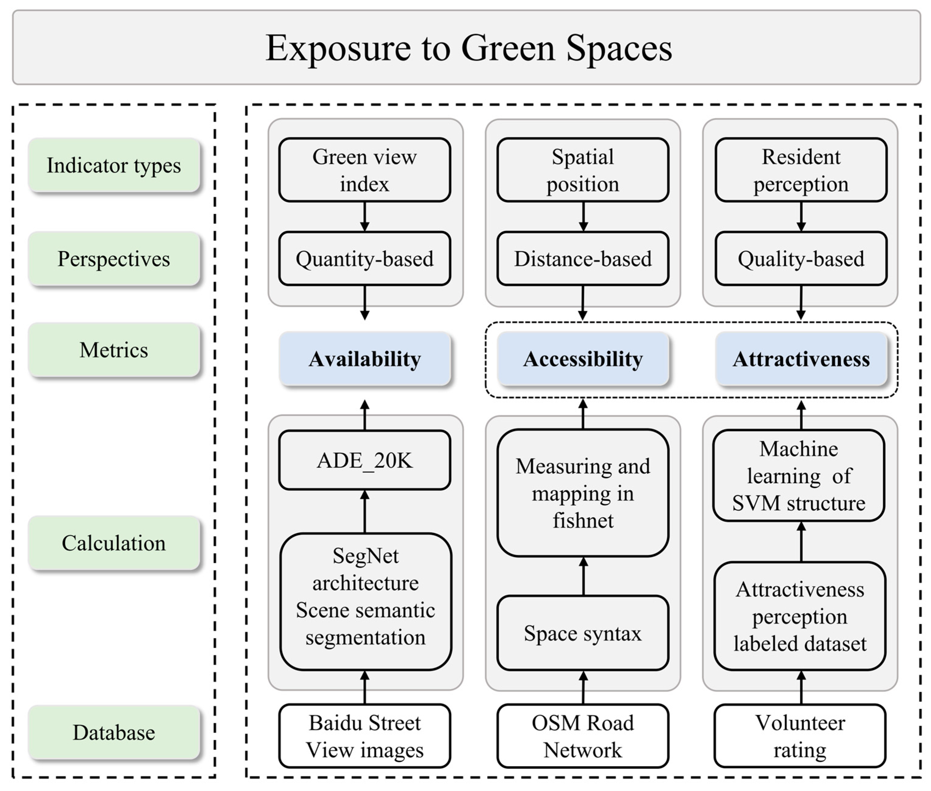
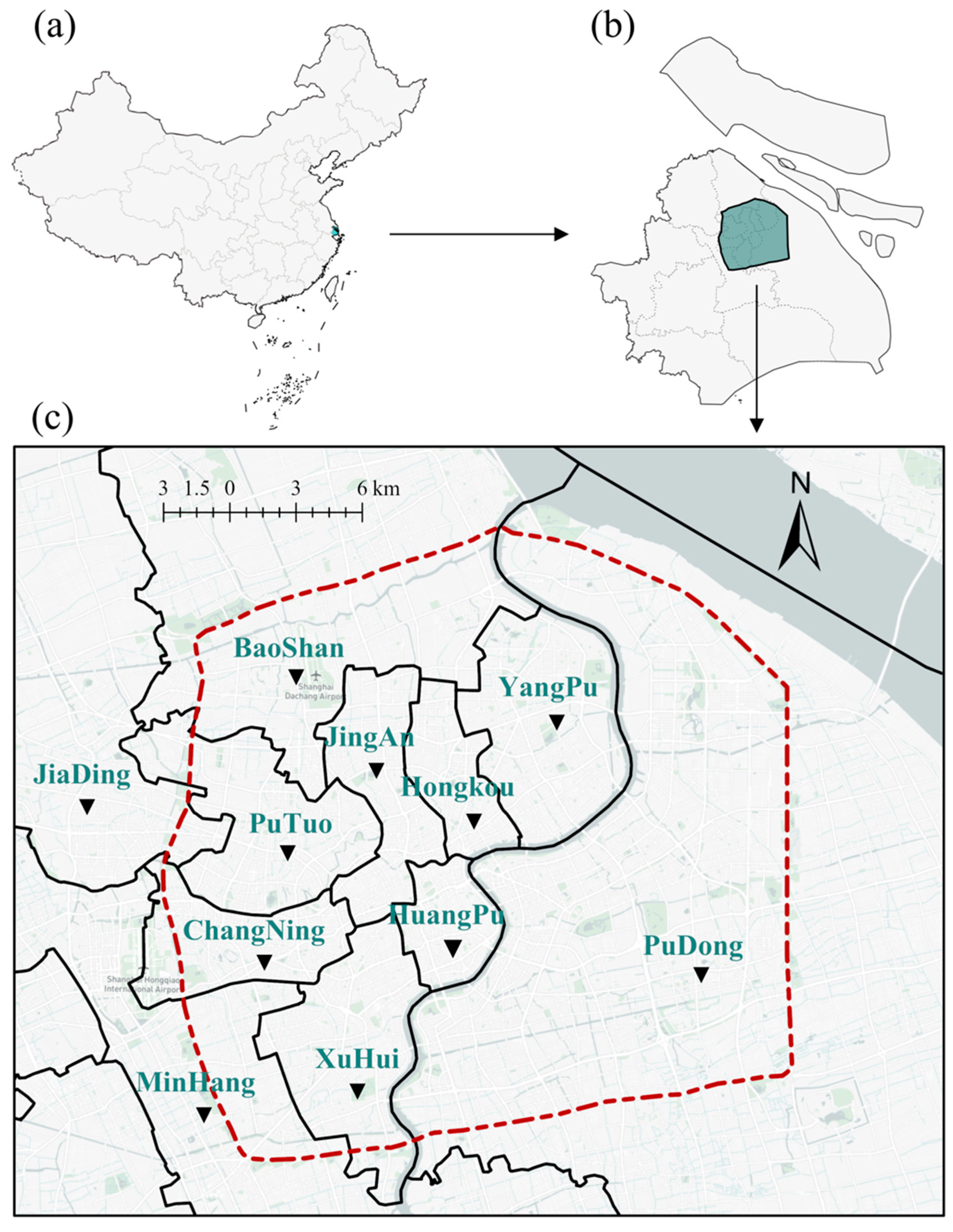
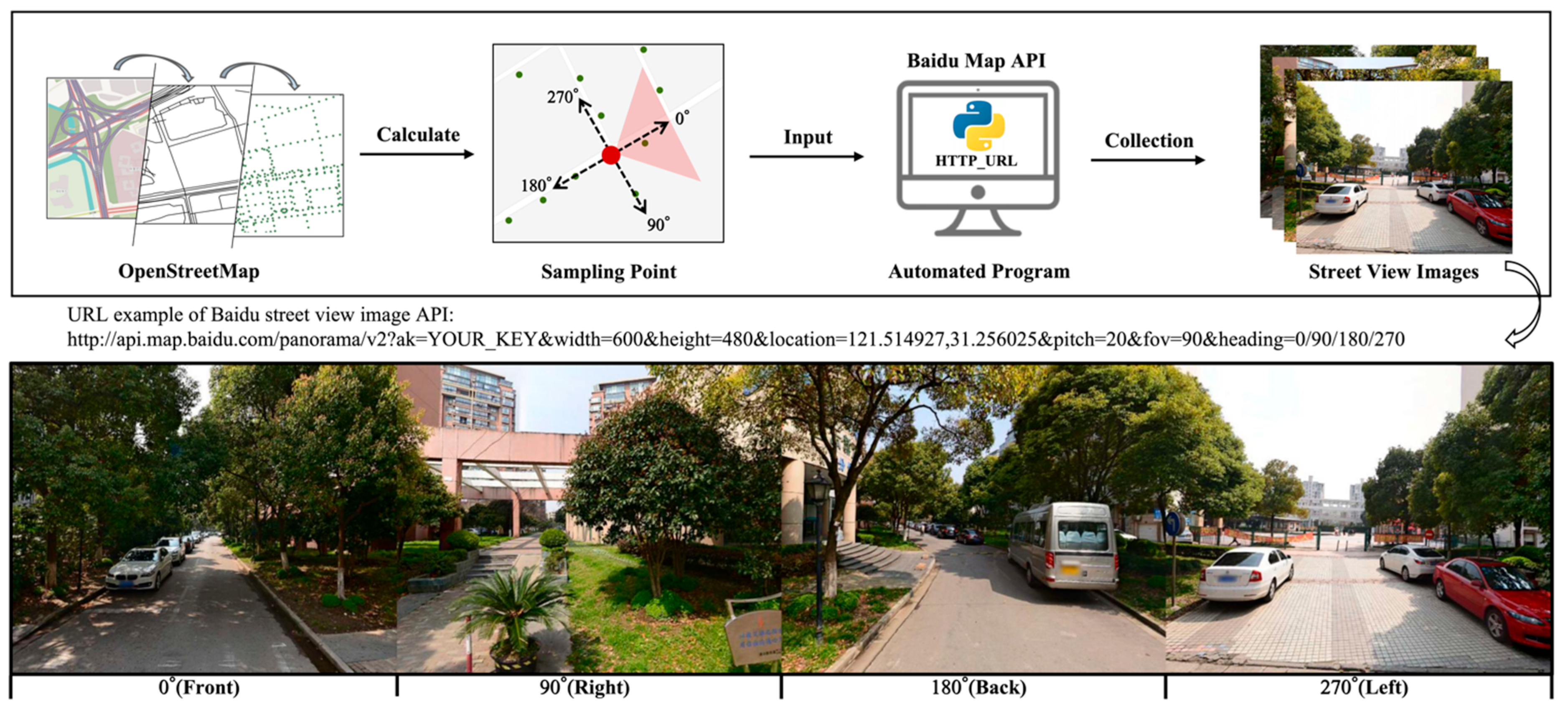
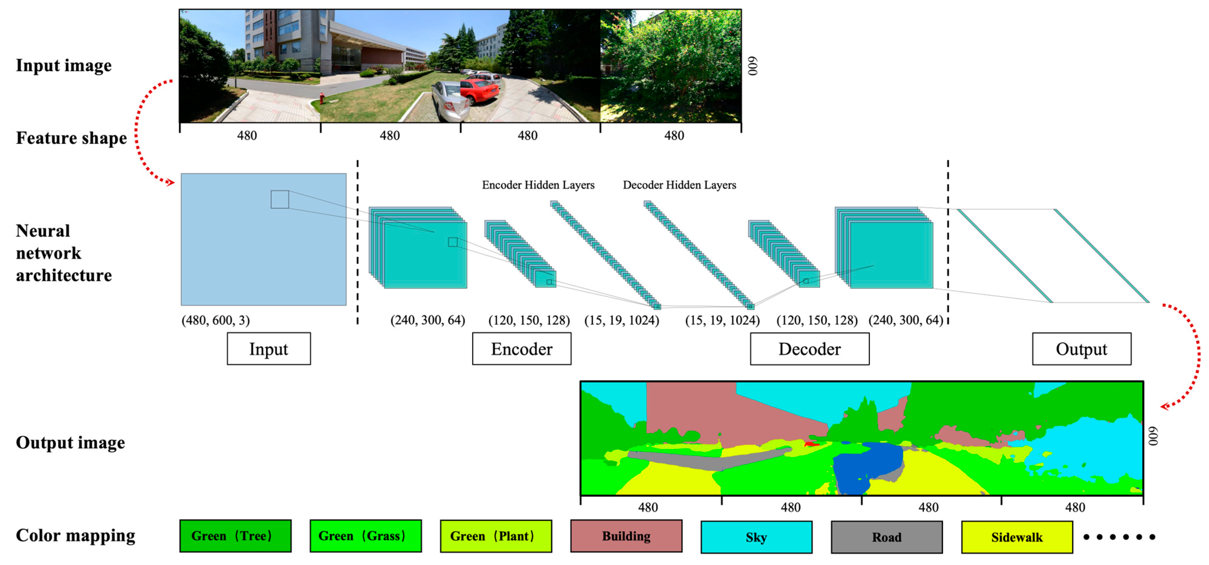

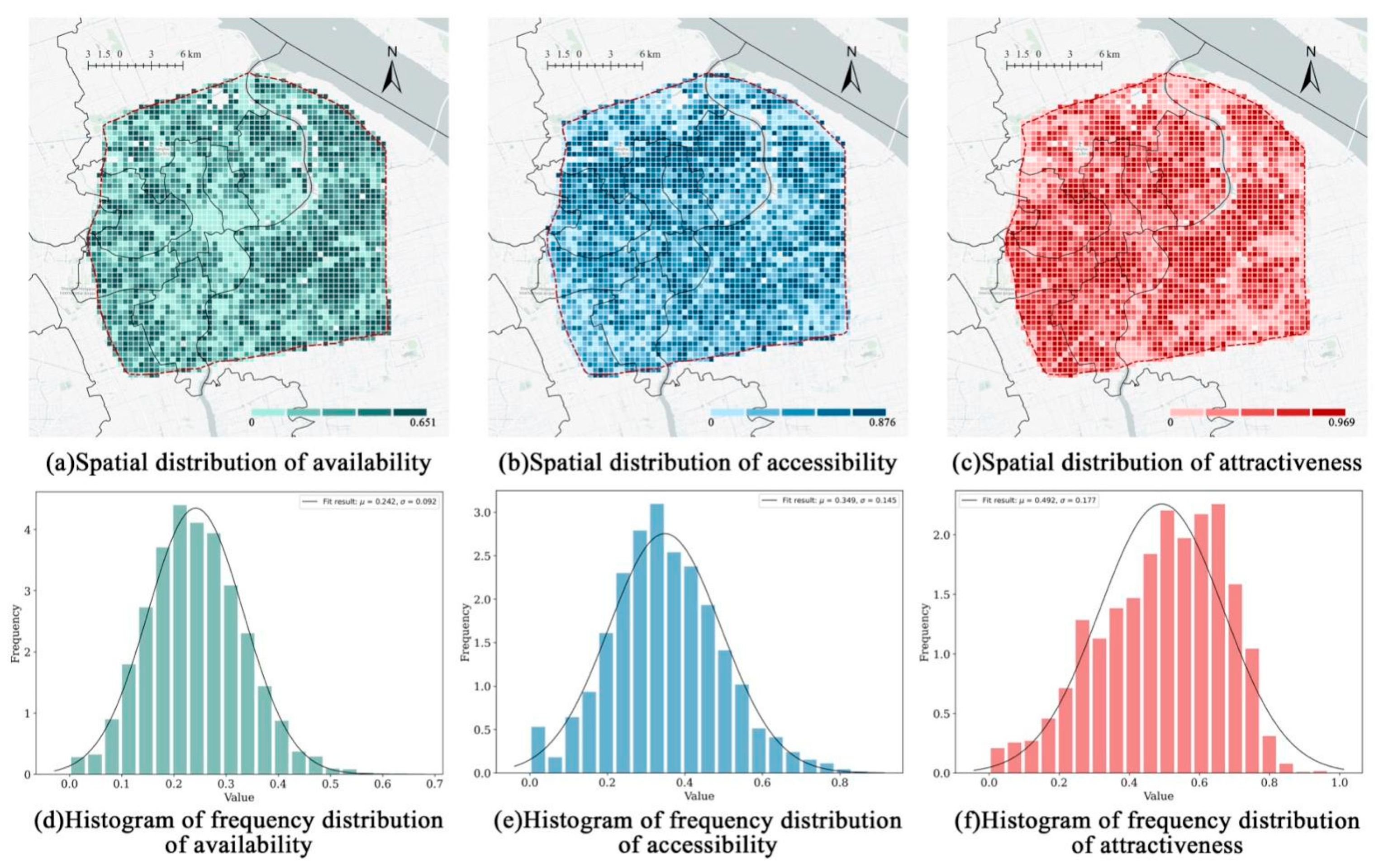
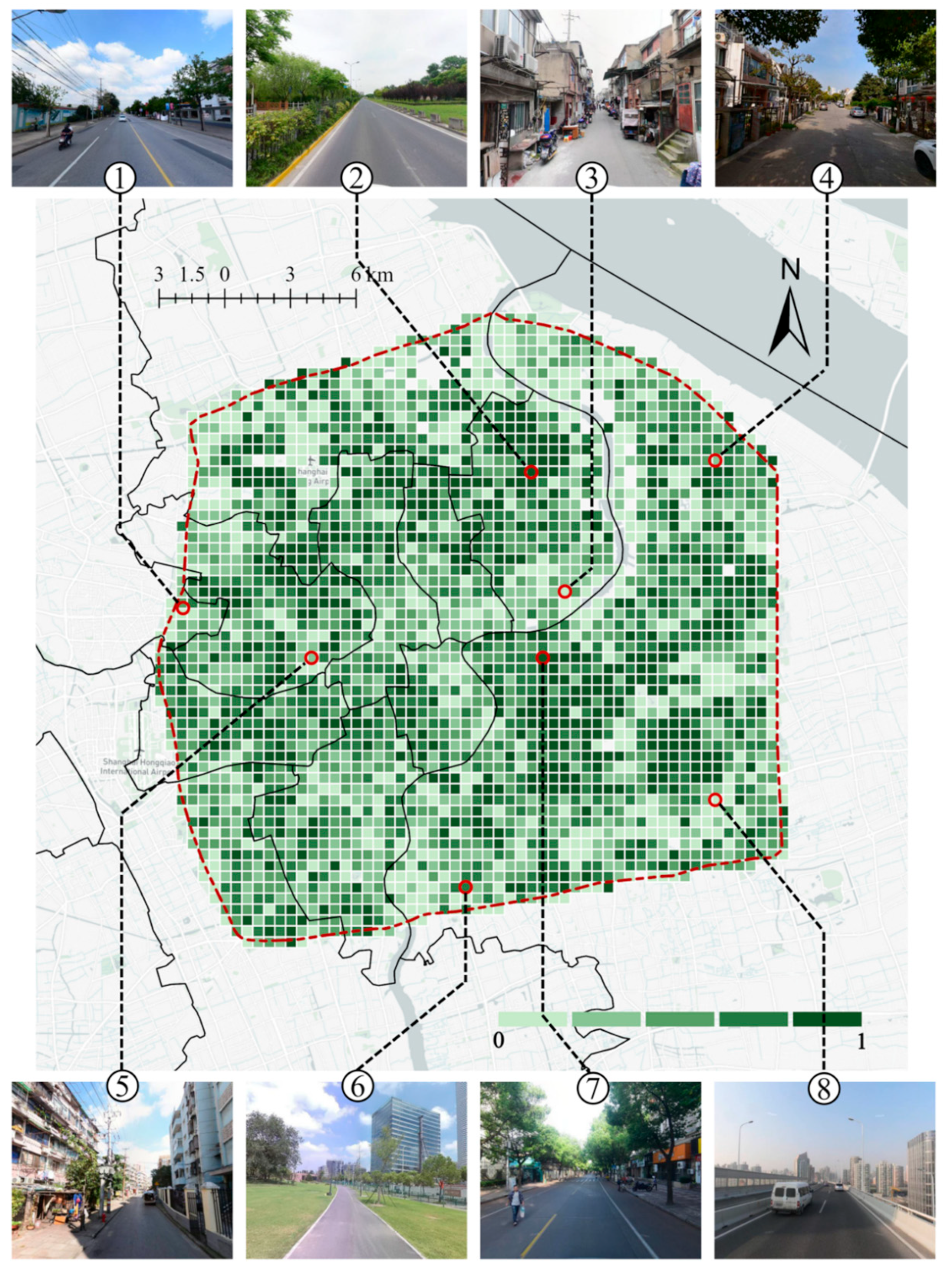
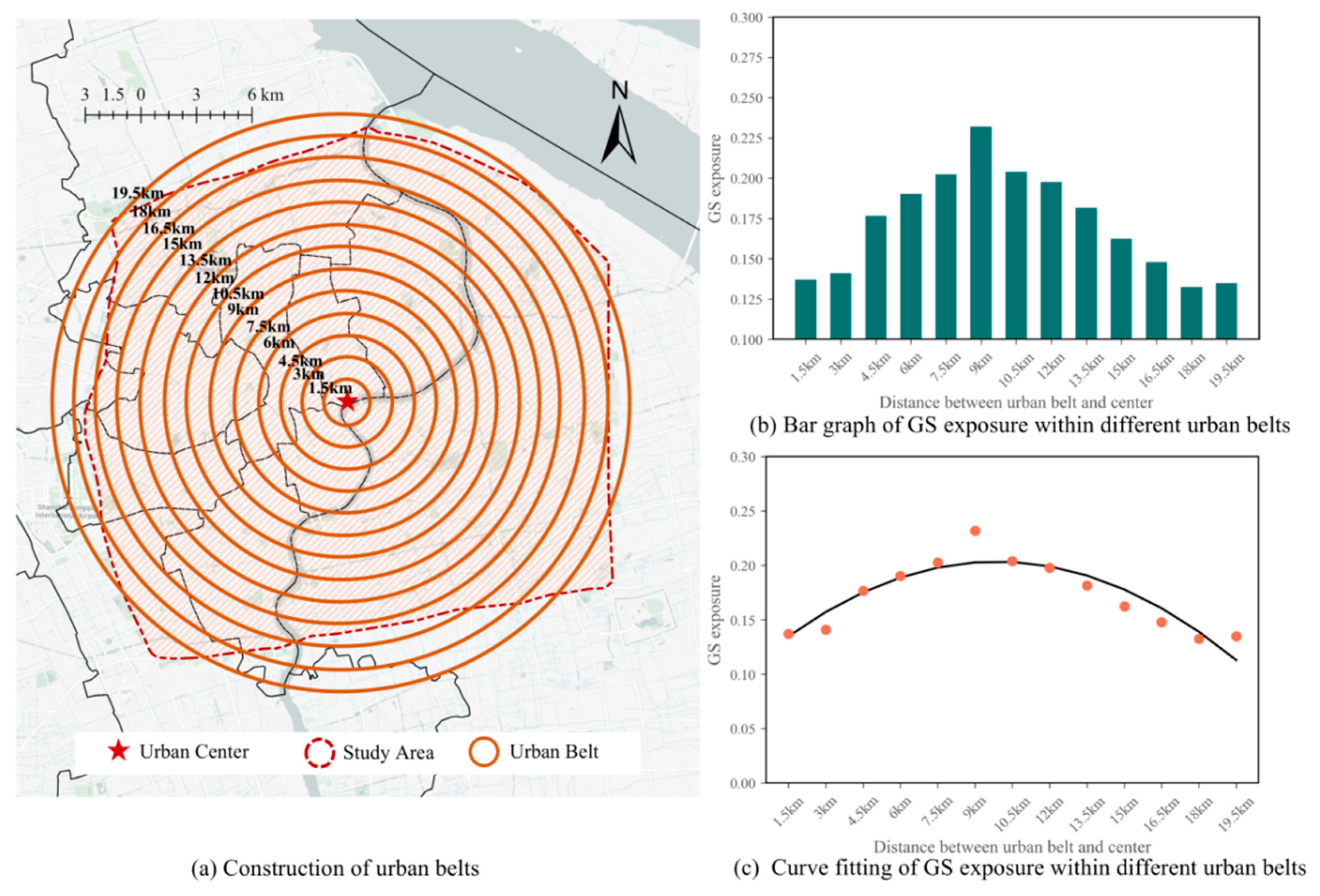
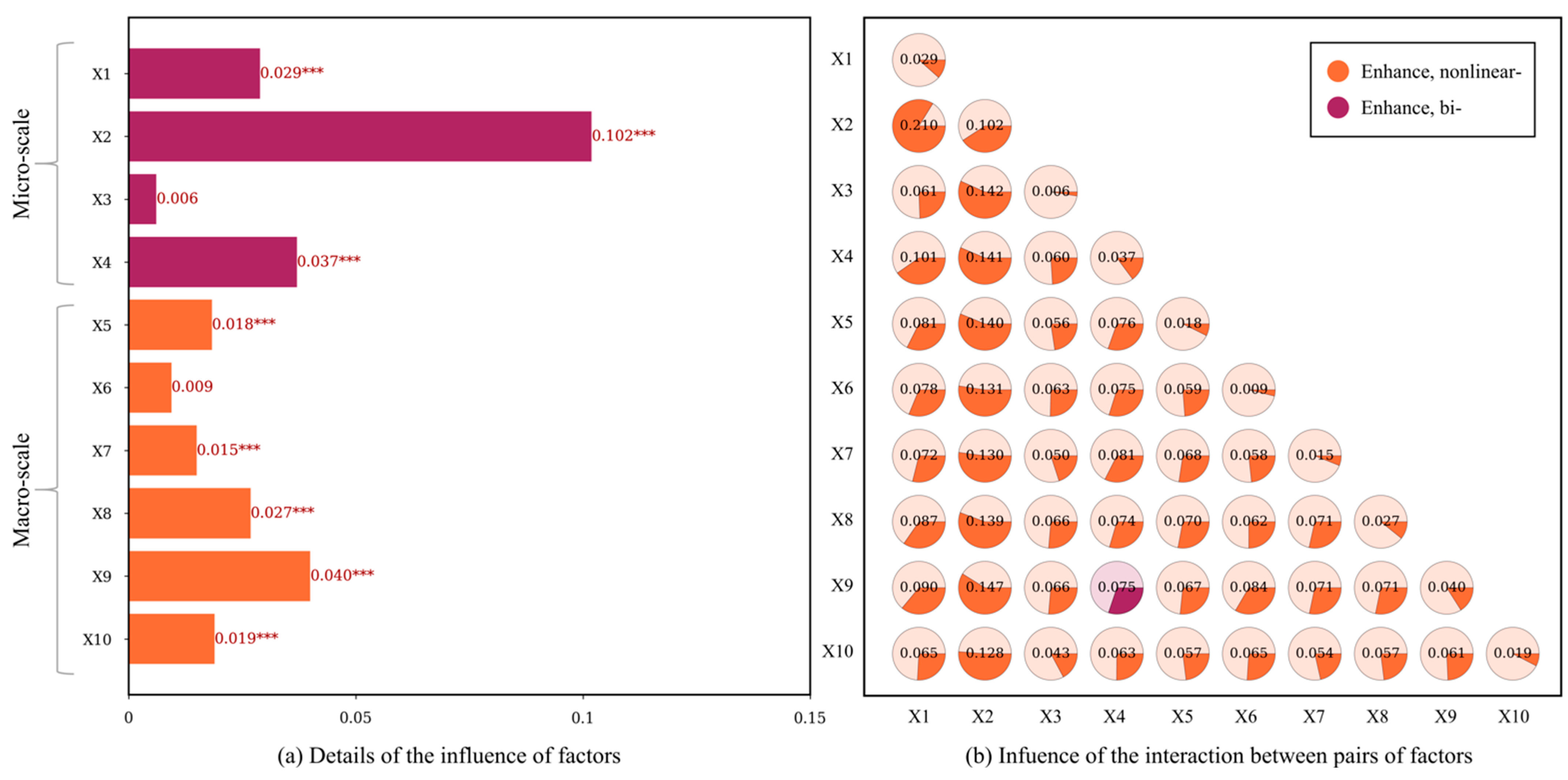
Disclaimer/Publisher’s Note: The statements, opinions and data contained in all publications are solely those of the individual author(s) and contributor(s) and not of MDPI and/or the editor(s). MDPI and/or the editor(s) disclaim responsibility for any injury to people or property resulting from any ideas, methods, instructions or products referred to in the content. |
© 2024 by the authors. Licensee MDPI, Basel, Switzerland. This article is an open access article distributed under the terms and conditions of the Creative Commons Attribution (CC BY) license (https://creativecommons.org/licenses/by/4.0/).