A Reliable DBH Estimation Method Using Terrestrial LiDAR Points through Polar Coordinate Transformation and Progressive Outlier Removal

Abstract

Diameter at breast height (DBH) is a crucial parameter for forest inventory. However, accurately estimating DBH remains challenging due to the noisy and incomplete cross-sectional points. To address this, this paper proposed a reliable DBH estimation method using terrestrial LiDAR points through polar coordinate transformation and progressive outlier removal. In this paper, the initial center was initially detected by rasterizing the convex hull, and then the Cartesian coordinates were transformed into polar coordinates. In the polar coordinate system, the outliers were classified as low and high outliers according to the distribution of polar radius difference. Both types of outliers were then removed using adaptive thresholds and the moving least squares algorithm. Finally, DBH was estimated by calculating the definite integral of arc length in the polar coordinate system. Twenty publicly available individual trees were adopted for the test. Experimental results indicated that the proposed method performs better than the other four classical DBH estimation methods. Furthermore, several extreme cases scanned using terrestrial LiDAR in practice, such as cross-sectional points with lots of outliers or larger data gaps, were also tested. Experimental results demonstrate that the proposed method accurately calculates DBH even in these challenging cases.

1. Introduction

Recent advancements in laser scanning technologies have made it possible to obtain accurate and detailed three-dimensional information about the structure of forests [1,2,3]. Terrestrial LiDAR (light detection and ranging), in particular, has emerged as a crucial method for monitoring forest resources due to its efficiency and precision [4,5]. The dense point clouds generated by this technology provide access to a wide range of forest attributes, including tree height [6], diameter at breast height (DBH, which is a measurement used in forestry to determine the diameter of a tree trunk at a standard height of 1.30 m above the ground) [7], crown width [8], tree volume [9], and above-ground biomass (AGB, which is an important metric used in forestry, ecology, and environmental studies to assess the carbon sequestration capacity of forests and vegetation) [10,11,12]. DBH, in particular, plays a vital role in forest inventory as it can be used to estimate various other tree metrics, such as tree height [13,14], wood volume [15], and foliage area [16]. Furthermore, DBH is also a key parameter in many allometric models used for AGB estimation [17,18].

Traditional methods for measuring DBH typically rely on calipers or tapes, which are inefficient and labor-intensive [19]. Moreover, manual visual measurements are prone to errors [4]. In contrast, terrestrial LiDAR offers an accurate and non-destructive solution for estimating DBH [20]. The methods using terrestrial LiDAR can be classified into three categories: DBH estimation based on regular geometry, DBH estimation by simulating manual measurement, and DBH estimation based on the quantitative structure model (QSM). The first two categories generally calculate DBH directly from point clouds, while the last category relies on the built individual tree models to achieve DBH values [4].

In terms of the DBH estimation methods based on regular geometry, circle fitting [21,22,23,24,25] and cylinder fitting [26,27,28] are two typical forms for calculating the DBH. Circle fitting methods involve selecting a slice of points and estimating the corresponding circle center and radius using techniques such as least squares fitting [21], random sample consensus (RANSAC) [29,30,31,32], and Hough transform [4,33]. For example, Reddy et al. [32] used the RANSAC algorithm for circle fitting, while Liu et al. [30] used RANSAC to calculate DBHs at different tree heights and removed wrongly calculated values based on the PauTa criterion to obtain accurate estimates. Panagiotidis et al. [34] applied a least squares circle fit algorithm in combination with hierarchical cluster analysis for DBH extraction. Koren et al. [35] compared five different circle fitting methods for DBH estimation and found that all four methods, except for the Monte Carlo method, tended to underestimate the DBH. Koren et al. [24] found that varying the thickness from 10 cm to 100 cm resulted in significant changes in calculated DBHs. Other factors such as range and angular errors of terrestrial LiDAR also have a significant impact on circle fitting results, as demonstrated by Wang et al. [6] in their experiments.

Cylinder fitting is similar to circle fitting but avoids selecting a specific layer of points [36]. Most circle fitting techniques can be applied to cylinder fitting as well. For example, Panagiotidis and Abdollahnejad [37] employed the RANSAC algorithm with a cylinder fitting strategy using points from cross-sectional areas and used the estimated the DBH for stem volume calculation. Srinivasan et al. [28] applied cylinder fitting to different height bins and calculated the average diameter of different directions to retrieve the DBH.

In summary, DBH estimation based on regular geometry assumes that the cross-section points of the stem are distributed in a circular or cylindrical shape. These methods have simple principles and are easy to implement. However, both circle fitting and cylinder fitting methods are sensitive to outliers, which can lead to incorrect DBH estimation results when dealing with noisy points or cross-section points with data gaps.

The second type of DBH estimation method relies on simulating manual measurement. Instead of assuming a regular geometry for the stem profile, these methods simulate the process of manual measurement using a tape [38]. As a result, these methods can be applied to different shapes of stem profiles and are more applicable in real-world scenarios. In this kind of method, convex hull points are generally detected initially [39]. You et al. [40] applied B-spline curves to interpolate the convex hull points and simulate the path of the tape. Subsequently, the DBH could be calculated using the calculated path length along the interpolated smooth curve. However, the extraction of convex hull points is easily influenced by outliers at the outermost points. In order to obtain more accurate DBH estimation results, Stovall et al. [39] proposed a convex hull peeling method to gradually remove outlying points. You et al. [38] proposed a caliper simulation method, where two parallel tangent lines were simulated as the caliper arms towards the convex hull points. By calculating the average distance between these lines, the DBH can be estimated. However, experimental results showed that this method tends to overestimate the DBH. In summary, the main advantage of these methods lies in their ability to handle irregular shapes of cross-section points of the stem. However, implementing these methods generally requires dense point clouds of high quality. Additionally, the simulation process is typically time-consuming [38].

The last category is QSM-based DBH estimation methods. In these methods, the QSM must be constructed for each individual tree as the first step. Several well-known individual tree modeling methods exist, including SimpleTree [41], TreeQSM [42] and AdTree [43]. It is important to note that all three of these methods are open-source, which facilitates the tree modeling process. DBH can be obtained as a byproduct of the modeling result. Ravaglia et al. [4] successfully applied SimpleTree for modeling and achieved satisfactory results in terms of DBH estimation. The mean errors in their study ranged from 1.03 cm to 3.34 cm. However, Ravaglia et al. [4] also mentioned that filtering is generally necessary to remove outliers and improve accuracy. Ye et al. [44] calculated DBH by building a quantitative structure model (QSM) for trees. However, their findings show that there are obvious deviations between QSM-based DBHs and referenced DBHs. The main limitation of this kind of method is that the accuracy of DBH estimation heavily relies on the quality of the QSM construction result. If the modeling result is poor due to occluded tree points, obtaining accurate DBH estimates becomes challenging. As a result, QSM-based DBH estimation methods are generally not suitable for single-scanned tree points, which are highly influenced by occlusion.

To sum up, data gaps caused by occlusion and outliers are the two main factors affecting the accuracy of DBH estimation regardless of the chosen DBH estimation method. Although some researchers have attempted to address these issues, occlusion and noisy points still affect most methods. Therefore, there is an urgent need to develop more accurate and robust DBH estimation methods. In this study, the Cartesian coordinates of cross-section points are first transformed into polar coordinates. This transformation is performed because points in polar coordinates are distributed in a wave-like pattern, which facilitates outlier detection through curve fitting. The noisy points are then classified as high or low outliers and removed separately using adaptive threshold filtering and the moving least squares algorithm. Finally, DBH is estimated based on the definite integral of arc length in the polar coordinate system.

2. Materials and Methods

2.1. Datasets

This study selected 20 individual trees from the terrestrial LiDAR datasets provided by Liang et al. [45]. These datasets were obtained in Evo, Finland (61.19° N, 25.11° E), using a Leica HDS6100 terrestrial laser scanner (Leica Geosystems AG, Heerbrugg, Switzerland). The scanner has a scanning view of 360° × 310° and a distance measurement accuracy of ±2 mm. Each individual tree was manually segmented from sample plots using an open-source visualization software called CloudCompare V2.13, and point clouds were scanned under different forest environments. Specifically, these 20 tree samples were chosen from three different forest plots measuring 32 by 32 m each. These plots contain a variety of tree species, including Scots pine, Norway spruce, silver birch, and downy birch. In each plot, both single-scan and multi-scan modes were used to capture the individual tree points. In the multi-scan mode, five scans were carried out within each plot: one at the center and four in the four quadrant directions.

The DBH values were measured manually using steel calipers at two perpendicular directions on-site. The mean value of these two measurements was considered the referenced DBH. In ideal conditions, the segmented points at breast height should be complete for each individual tree, as shown in Figure 1a,b. However, there are often outliers caused by the instrument itself or adjacent shrubs, which can introduce errors in DBH calculation, as shown in Figure 1c,d. Additionally, due to limitations in scanning view or occlusion, the segmented points at breast height may have data gaps, resulting in an incomplete circle-like shape, as shown in Figure 1e,f.

Among the selected 20 individual trees, all three cases mentioned above (complete points, noisy points, and incomplete points) were present. Therefore, the proposed method’s robustness against different scenarios can be tested.

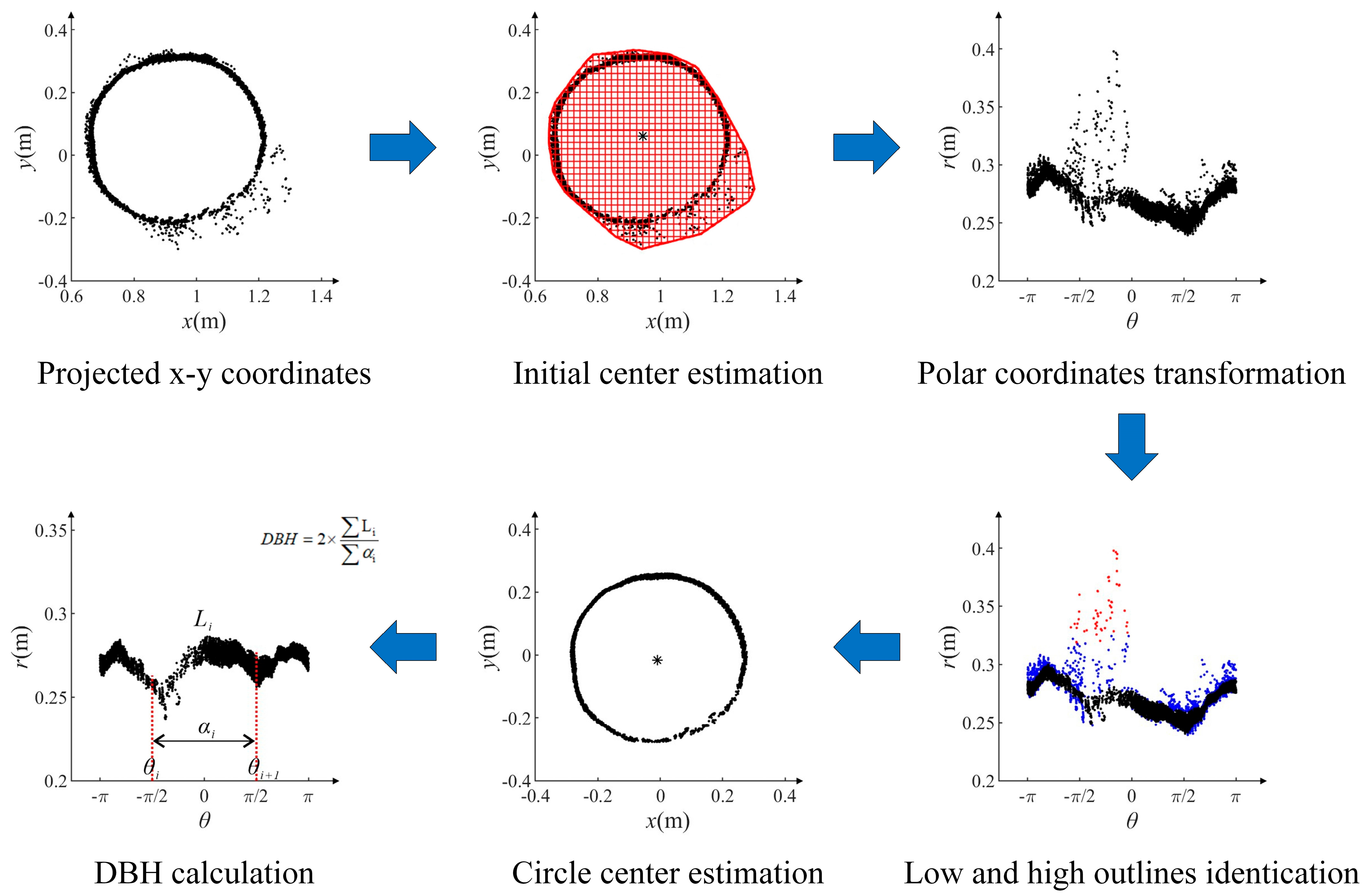
2.2. Methodology

The flowchart in Figure 2 illustrates the proposed method. DBH is commonly defined as the stem diameter at a distance of 1.30 m from the tree root. Therefore, a segment of point clouds between 1.25 m and 1.35 m from the tree root is initially segmented. These points are then projected onto a horizontal plane. To convert the points from Cartesian coordinates into polar coordinates, an initial center is estimated by rasterizing the convex hull formed by x–y coordinates. After transforming them into polar coordinates, it becomes apparent that there are outliers caused by the instrument itself or adjacent shrubs. These outliers significantly affect the accuracy of DBH estimation and are defined in this paper as high and low outliers. High outliers are removed using an adaptive threshold, while low outliers are identified through iterative use of the moving least squares algorithm. Once the outliers are removed, the polar coordinates are transformed back to Cartesian coordinates. Subsequently, a rough estimate of the circle center can be obtained using the least squares algorithm. Based on this newly calculated center, the Cartesian coordinates are further transformed into polar coordinates. Finally, DBH can be estimated by calculating the definite integral of arc length in the polar coordinate system. In summary, this paper includes three main steps: (i) fast initial center estimation by rasterizing convex hull, (ii) polar coordinate transformation and high/low outlier identification, and (iii) DBH estimation based on the definite integral of arc length.

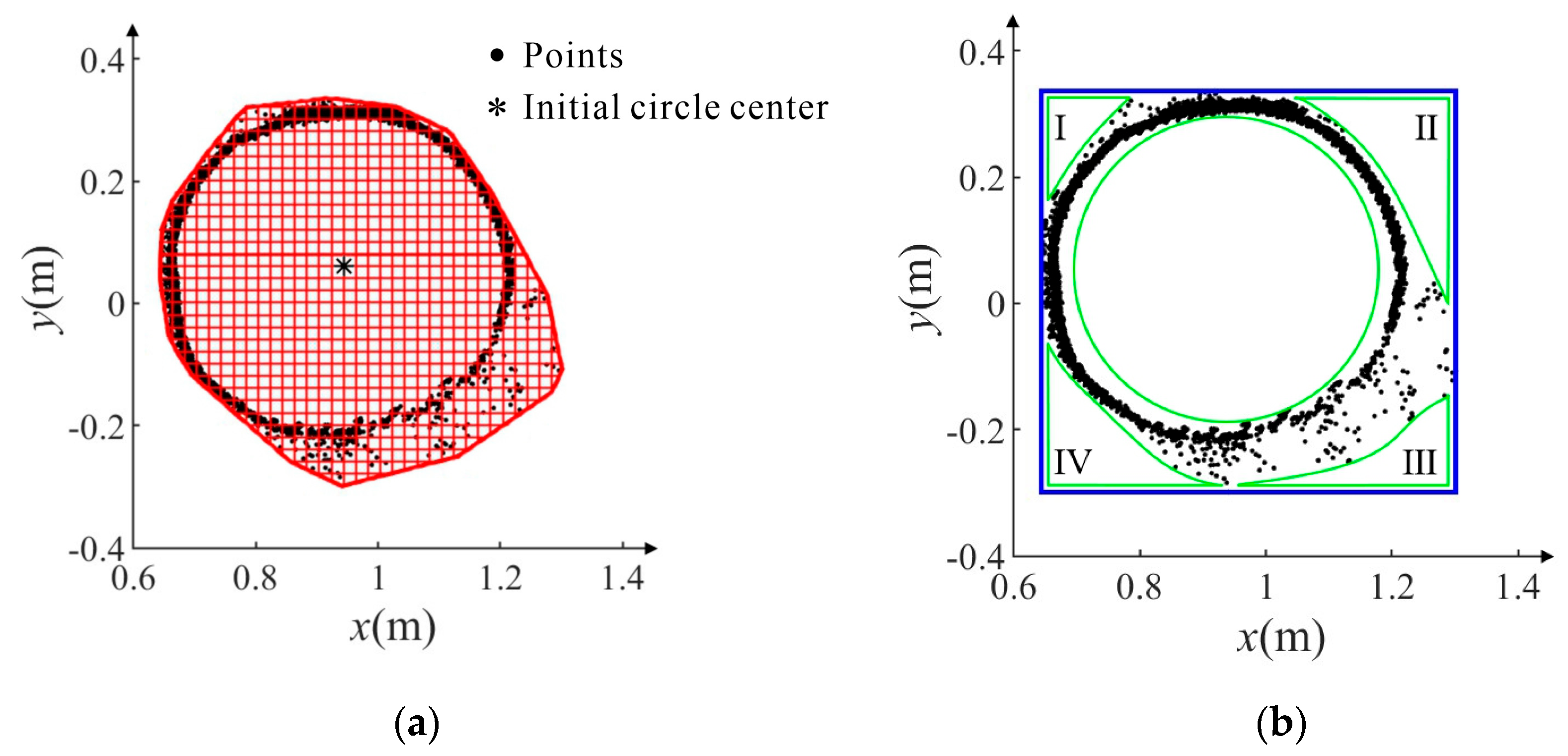
2.2.1. Fast Initial Center Estimation by Rasterizing Convex Hull

The cross-section of the stem usually resembles a circle shape, which allows the DBH to be estimated as the diameter of a fitting circle. Ideally, if the projected horizontal points used for DBH calculation were perfectly distributed along the circle (Figure 3a), their distances from the center would be equal. In other words, their polar radii should be equal when transforming Cartesian coordinates into polar coordinates with the circle center selected as the pole (Figure 3b). However, in practice, the sliced points of the stem do not strictly form a circle shape, as shown in Figure 3c. As a result, the corresponding transformed polar coordinates exhibit a wave-like curve, as shown in Figure 3d.

To transform Cartesian coordinates into polar coordinates, it is crucial to first locate the circle center as the pole. In general, the center should lie within the sliced points. To exclude incorrectly detected centers outside the sliced points, this paper restricts the location of the center within the minimum convex polygon (red line in Figure 4a) formed by applying the convex hull algorithm. Additionally, this area is further divided into rasterized grids for quick center identification. Typically, the center should be located at the farthest point from all projected horizontal points within the convex hull. Therefore, by traversing each grid point individually, the grid point with the farthest distance from the projected points is selected as the initial center (shown as a black asterisk in Figure 4a). It is important to note that if no restrictions are imposed on locating the center point within the convex hull, then the farthest grid point may fall outside of the sliced points. As illustrated in Figure 4b, this farthest grid point may be located in areas I, II, III, or IV. This is why building a convex hull is necessary to confine the center point within the minimum convex polygon.

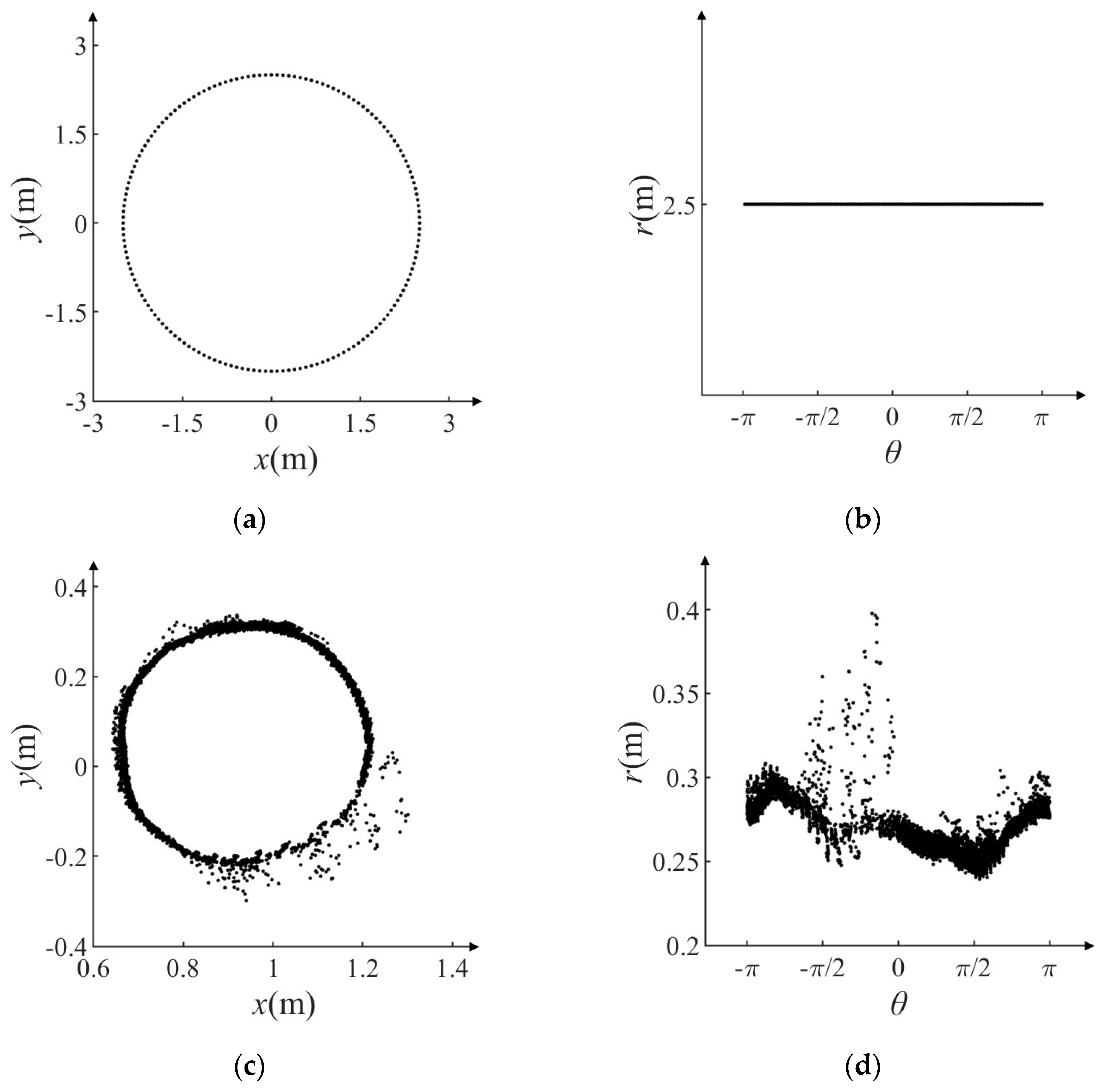
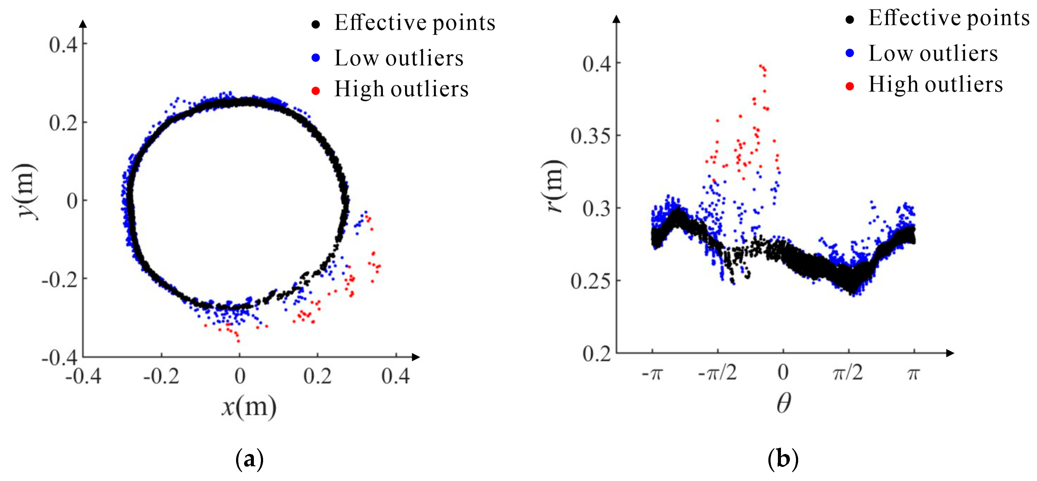
2.2.2. Polar Coordinate Transformation and High/Low Outlier Identification

Once the initial center is obtained, the horizontal points can be centralized. Using Equation (1), the Cartesian coordinates can then be transformed into polar coordinates.

$$\left\{\begin{array}{l}r=\sqrt{x^2+y^2}\hfill \\ \theta =\arctan \left(y/x\right)\hfill \end{array}\right.$$

(1)

where $r$ is the polar radius, while $\theta$ is the polar angular. Ideally, all circle points should have equal $r$ values. However, due to the influence of the instrument itself or adjacent shrubs, as shown in Figure 5a, the transformed polar coordinates generally take on a wave-like shape with several outliers, as depicted in Figure 5b.

This paper categorizes these outliers into two groups: high and low outliers. High outliers are those points that deviate significantly from the wave-like curve, represented by the red points in Figure 5b. Conversely, low outliers are points that are mixed in with the wave-like curve, illustrated by the blue points in Figure 5b. The classification rule is defined by Equation (2).

$$\left\{\begin{array}{l}if \Delta r_i\ge \delta , p_i\in high outlier\hfill \\ if \Delta r_i<\delta \& abs\left(r_{p_i}-{\widehat{r}}_{p_i}\right)\ge \eta , p_i\in low outlier\hfill \end{array}\right.$$

(2)

where $\Delta r_i$ is the difference between the point and minimum polar radius in each section, as shown in Figure 6. Here, each section is divided by 0.05 radians. Due to the existence of outliers, the values of $\Delta r_i$ will be fluctuant. $\delta$ is a self-adaptive threshold, which will help remove the point with a higher $\Delta r_i$. $r_{p_i}$ is the polar radius of $p_i$, while ${\widehat{r}}_{p_i}$ is the polar radius correspondingly fitted by the moving least squares algorithm. $\eta$ is a self-adaptive threshold that is used for identifying the low outliers. Both $\delta$ and $\eta$ can be calculated self-adaptively in this paper.

As mentioned above, $\Delta r_i$ will be varied due to the existence of outliers. Some points with a larger $\Delta r_i$ will be detected as high outliers. Thus, it is important to calculate the threshold $\delta$. This paper first calculates the maximum polar radius difference, $\Delta r_i^{\max }$, in each section, that is, $S=\left\{\Delta r_1^{\max }\cdots ,\Delta r_i^{\max }\cdots ,\Delta r_n^{\max }\right\}$, which is distributed as shown in Figure 7.

From Figure 7, it can be found that there are several extremely larger $\Delta r_i^{\max }$ values. Here, this paper excludes these larger $\Delta r_i^{\max }$ values based on the threshold calculated as $q_1+1.5\Delta q$. $q_1$ represents the upper quartile, while $\Delta q$ is the interquartile range. After excluding the larger $\Delta r_i^{\max }$, a new set can be achieved, that is, $S^{\prime }=\left\{\Delta r_1^{\max }\cdots ,\Delta r_i^{\max }\cdots ,\Delta r_m^{\max }\right\}$, $m\le n$. Then, the data set, $S^{\prime }$, is sorted from smallest to largest. Subsequently, the difference between the two successive data (eg., $\Delta r_i^{\max }$ and $\Delta r_{i+1}^{\max }$) is calculated as $\sigma r_i$. Hereafter, a new set, $S^{″}=\left\{\sigma r_1\cdots ,\sigma r_i\cdots ,\sigma r_{m-1}\right\}$, can be achieved. This paper further calculates the mean value ($\overline{\sigma r}$) and standard deviation ($\widetilde{\sigma r}$) of $S^{″}$ and detects the first $\sigma r_i$ that is larger than $\overline{\sigma r}+3\widetilde{\sigma r}$. Finally, the corresponding $\Delta r_i^{\max }$ is set as the high outlier detection threshold, that is, $\delta =\Delta r_i^{\max }$. For instance, if $\sigma r_5$ is the first value larger than $\overline{\sigma r}+3\widetilde{\sigma r}$, $\delta$ is equal to $\Delta r_5^{\max }$.

As shown in Figure 5b, there are several low outliers mixed with the wave-like curve. This paper adopted the moving least squares algorithm to delete these low outliers. As shown in Figure 8a, the moving window in this paper is set to four neighboring sections. The fitted polar radius for $p_i$ can be calculated as ${\widehat{r}}_{p_i}$ using the points fallen within the moving window. In terms of ${\widehat{r}}_{p_i}$, all the differences between the polar radiuses and ${\widehat{r}}_{p_i}$ can be calculated as shown in Figure 8b. From Figure 8b, the upper quartile, $Q_1$, and interquartile range, $\Delta Q$, can be calculated. In this paper, $\eta$ is set to $Q_1+1.5\Delta Q$, that is, if the difference between the polar radius and ${\widehat{r}}_{p_i}$ is larger than $\eta$, the corresponding point will be identified as a low outlier.

2.2.3. DBH Calculation Based on the Definite Integral of Arc Length

After removing all high and low outliers, “clean” polar coordinates can be obtained, as shown in Figure 9a. These polar coordinates can also be converted back into Cartesian coordinates, as demonstrated in Figure 9b. It can be observed from Figure 9b that the point distribution is closer to a circle. By employing the least squares fitting algorithm, a rough center can be estimated and represented by the red fork in Figure 9b. It should be noted that this paper refers to this estimated center as a “rough center” because it is based on an initial center (the black asterisk point shown in Figure 4a). This initial center is generally not accurate. To achieve precise DBH estimation results, the newly calculated center depicted in Figure 9b is used to transform the Cartesian coordinates presented in Figure 9b into polar coordinates, as illustrated in Figure 9c. Consequently, DBH can be estimated according to Equation (3).

$$\left\{\begin{array}{l}DBH=2\frac{L}{\alpha }\hfill \\ L={\displaystyle \sum _{i=1}^n{L}_i},\alpha ={\displaystyle \sum _{i=1}^n{\alpha }_i}\hfill \end{array}\right.$$

(3)

$$L_i={\displaystyle {\int }_{{\theta }_i}^{{\theta }_{i+1}}\sqrt{r^2+{\left(\frac{dr}{d\theta }\right)}^2}d\theta }$$

(4)

where $L$ is the arc length, while $\alpha$ is the corresponding radian. In complex forest environments, it is generally hard to obtain complete stem points due to the scanning angle especially when adopting single-scanning mode. As a result, the wave-like curve is generally fragmentized as shown in Figure 9d. Then, the arc length, $L$, can be calculated by summing each fragmentized arc length, $L_i$, while $L_i$ can be calculated based on the definite integral of arc length from ${\theta }_i$ to ${\theta }_{i+1}$ according to Equation (4).

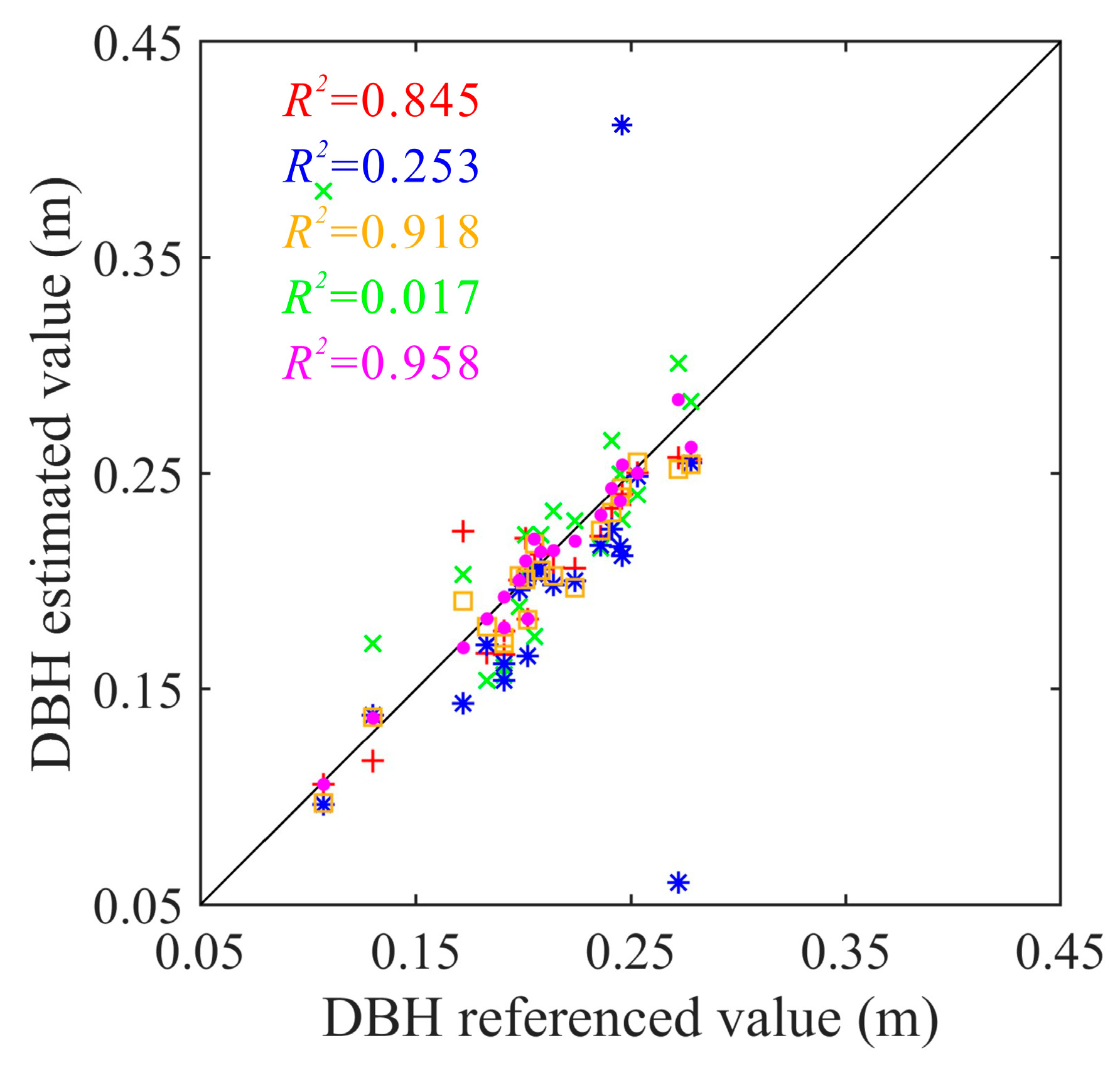
3. Experimental Results

To visually demonstrate the effectiveness of this method, six out of the twenty DBH estimation results were tabulated in Figure 10. These six cross-sectional points correspond to the six trees depicted in Figure 1. From Figure 10, it can be found that in terms of complete cross-sectional points, the proposed method can fit a circle-like shape well (red circles in Figure 10a,b). In terms of noisy cross-sectional points, although there are many outliers in Figure 10c,d, the proposed method can estimate the DBH well. This is because the proposed method can exclude outliers effectively in the polar coordinate system. In terms of incomplete cross-sectional points, as depicted in Figure 10e,f, although only small part of cross-sectional points remained, the proposed method achieved satisfactory DBH estimation results.

This paper estimated all the DBHs for these 20 trees. The estimated results were shown in Figure 11. Meanwhile, this paper also calculated the DBH estimation results using four other methods proposed by Olofsson et al. [31], Liu et al. [33], Liu et al. [30], and Mokroš et al. [46]. Olofsson et al. [31] introduced a modified RANSAC DBH estimation method. They made several adjustments to the traditional RANSAC approach. Firstly, they deemed a circle invalid if it had more than 1% of the points inside. Secondly, they restricted the range of circle radii to be between 2 cm and 30 cm, considering circles with smaller or larger radii invalid. Liu et al. [33] proposed a random Hough transform DBH estimation method. In their approach, they randomly selected three non-collinear points with a minimum spacing of 0.02 m between them. Each set of three points was then used to fit a circle, and only circles that satisfied the radius constraints were considered in the Hough parameter space. Liu et al. [30] calculated DBH values at different heights. They applied the RANSAC algorithm for DBH estimation on each set of sliced points. By detecting incorrectly calculated DBH values based on the PauTa criterion, they obtained the final DBH estimation. Mokroš et al. [46] obtained the DBH estimation results using a cylinder fitting technique. In their method, the cylinder element was obtained at 1.3 m above the ground. From Figure 11, it can be found that compared with other methods, there are more points of the proposed method that closely surround the 1:1 line. This means that the estimated DBH values are close to the referenced DBH values. This paper calculated the coefficients of determination ($R^2$) between estimated DBH values and reference values of different methods. It is easy to find that the method in this paper performed much better than the other four methods. Thus, it can be concluded that this paper’s method can achieve better performance in DBH estimation.

To quantitatively evaluate the performance of this method, five accuracy indicators were used for assessing the performance of the proposed method, including bias, relative bias, root mean squared error, relative root mean squared error, and the concordance correlation coefficient. They are defined in Equations (5)–(9):

$$Bias=\frac{{\displaystyle \sum _{i=1}^N(DB{H}_{est}^i-DB{H}_{ref}^i)}}{N}$$

(5)

$$rBias=\frac{Bias}{\overline{DB{H}_{ref}}}\times 100\%$$

(6)

$$RMSE=\sqrt{\frac{{\displaystyle \sum _{i=1}^N{(DB{H}_{est}^i-DB{H}_{ref}^i)}^2}}{N}}$$

(7)

$$rRMSE=\frac{RMSE}{\overline{DB{H}_{ref}}}\times 100\%$$

(8)

$$\left\{\begin{array}{l}CCC=\frac{\frac{2}{N}{\displaystyle \sum _{i=1}^N(DB{H}_{est}^i-\overline{DB{H}_{est}})(DB{H}_{ref}^i-\overline{DB{H}_{ref}})}}{{\sigma }_{est}^2+{\sigma }_{ref}^2+{(\overline{DB{H}_{est}}-\overline{DB{H}_{ref}})}^2}\hfill \\ {\sigma }_{est}^2=\frac{1}{N}{\displaystyle \sum _{i=1}^N{(DB{H}_{est}^i-\overline{DB{H}_{est}})}^2}\hfill \\ {\sigma }_{ref}^2=\frac{1}{N}{\displaystyle \sum _{i=1}^N{(DB{H}_{ref}^i-\overline{DB{H}_{ref}})}^2}\hfill \end{array}\right.$$

(9)

where $Bias$, $rBias$, $RMSE$, $rRMSE$, and $CCC$ represent bias, relative bias, root mean squared error, relative root mean squared error, and the concordance correlation coefficient, respectively. $DB{H}_{est}^i$ and $DB{H}_{ref}^i$ represent the i-th estimated and reference DBH values. $\overline{DB{H}_{est}}$ and $\overline{DB{H}_{ref}}$ represent the mean estimated and reference DBH values. $N$ is the number of trees for DBH estimation.

The mean accuracy metric calculation results are tabulated in

Table 1. Accuracy metrics of different methods.

DBH Estimation Methods	Bias (mm)	rBias (%)	RMSE (mm)	rRMSE (%)	CCC
Olofsson et al. [31]	−5.67	−2.70	17.54	8.36	0.91
Liu et al. [33]	−7.21	−3.44	14.00	6.67	0.94
Liu et al. [30]	14.10	6.72	65.19	31.06	0.12
Mokroš et al. [46]	−0.41	−0.20	30.91	14.73	0.76
The proposed method	−0.75	−0.36	8.68	4.13	0.98

. It is easy to find that the proposed method performs much better than the other methods in terms of RMSE, rRMSE, and CCC. The Bias of the proposed method is −0.75 mm, which is only a little larger than the results by Mokroš et al. [46]. However, the RMSE and rRMSE values of Mokroš et al. [46] are more than three times those of the proposed method. This means that the method by Mokroš et al. [46] cannot achieve satisfactory performance in different DBH estimation cases. Comparatively, the proposed method achieved the smallest RMSE and rRMSE values. This indicates that the proposed method has stronger robustness. When it comes to CCC, the CCC of the proposed method is 0.98, which is much closer to 1 than that of the other four methods. This means that the DBH values estimated in this paper are much closer to the referenced DBH values.

4. Discussion

To visually compare the performance of the proposed method in some extreme cases, such as when there are cross-sectional points with a huge amount of outliers and cross-sectional points with larger data gaps, several trees scanned in practice were used for testing. Different scenarios of cross-sectional points were chosen, including noisy, incomplete, and irregular ones, as displayed in Figure 12. The DBH estimation was carried out using five methods (that of Olofsson et al. [31], Liu et al. [33], Liu et al. [30], and Mokroš et al. [46], and the proposed method), with DBH values obtained from tape or caliper measurements serving as references. The results of the five methods and the referenced values are presented in Figure 12. When dealing with noisy cross-sectional points, it was observed that Liu et al. [33] incorrectly identified the circle, leading to an overestimated DBH value (Figure 12b). Olofsson et al. [31] and Mokroš et al. [46] provided underestimations (Figure 12a,d), while the proposed method yielded the closest estimate to the true value (Figure 12e). For incomplete points (Figure 12g–l), all methods except the proposed one tended to underestimate the DBH. Regarding irregular cross-sectional points, where points are not strictly distributed in circular shapes, the proposed method demonstrated superior accuracy compared with the other four methods (Figure 12q). Overall, based on the extreme cases illustrated in Figure 12, it can be concluded that the proposed method delivers satisfactory DBH estimation performance with strong robustness.

As can be seen from the discussion above, the proposed approach can produce satisfactory DBH estimation results for a variety of forest stand situations, including locations that are noisy, incomplete, or irregular. It must be acknowledged, nonetheless, that each of the aforementioned forest stands is made up of manually divided individual trees. Correct individual tree segmentation results are necessary for accurate DBH estimation.

Figure 13a depicts individual trees surrounded by dense low bushes or small trees. In this instance, obtaining correct individual tree segmentation results is tough, making reliable DBH estimation results much more difficult. To attain a satisfactory DBH estimation result, some ‘boosting’ processes should be added. As illustrated in Figure 13b, the normal vector constraint is first used to remove some of the leaves. Next, the DBSCAN clustering technique is used to retrieve various clustering object primitives, as shown in Figure 13c. The final stems were then extracted by analyzing the linear and height features of each object primitive, as shown in Figure 13d. After extracting the stems, DBH can be calculated using our proposed approach.

5. Conclusions

DBH plays a vital role in forest inventory, enabling accurate tree height estimation, AGB calculation, and more. However, estimating DBH remains challenging due to issues like low accuracy, particularly in the presence of noisy cross-sectional points and incomplete data. To enhance the effectiveness and robustness of DBH estimation, this paper introduces a reliable method using terrestrial LiDAR points through polar coordinate transformation and progressive outlier removal. In the proposed method, the initial center is first estimated by rasterizing the convex hull, and then the Cartesian coordinates are transformed into polar coordinates. Subsequently, outliers are identified as low or high outliers and gradually removed. Following outlier removal, the DBH is calculated based on the definite integral of arc length. In total, 20 publicly available individual trees were used for testing. The experimental results demonstrate that our proposed method consistently outperforms other methods across various accuracy indicators. The CCC value of the proposed method is 0.98, indicating that estimated DBH values closely align with the referenced DBH values. To further test the robustness of the proposed method, several extreme cases are adopted for testing. The proposed method successfully achieves accurate DBH estimations by progressively removing outliers and effectively resisting their impact. Compared with the other four methods, the proposed method achieved better performance in different DBH estimation cases. These results confirm that the proposed method demonstrates exceptional effectiveness and robustness in DBH estimation.

References

- Weiser, H.; Schaefer, J.; Winiwarter, L.; Krasovec, N.; Fassnacht, F.E.; Hoefle, B. Individual tree point clouds and tree measurements from multi-platform laser scanning in German forests. Earth Syst. Sci. Data 2022, 14, 2989–3012. [Google Scholar] [CrossRef]
- Li, J.; Wu, H.; Xiao, Z.; Lu, H. 3D modeling of laser-scanned trees based on skeleton refined extraction. Int. J. Appl. Earth Obs. Geoinform. 2022, 112, 102943. [Google Scholar] [CrossRef]
- Hui, Z.; Cheng, P.; Yang, B.; Zhou, G. Multi-level self-adaptive individual tree detection for coniferous forest using airborne LiDAR. Int. J. Appl. Earth Obs. Geoinform. 2022, 114, 103028. [Google Scholar] [CrossRef]
- Ravaglia, J.; Fournier, R.A.; Bac, A.; Vega, C.; Cote, J.; Piboule, A.; Remillard, U. Comparison of three algorithms to estimate tree stem diameter from terrestrial laser scanner data. Forests 2019, 10, 5997. [Google Scholar] [CrossRef]
- Zhu, X.; Skidmore, A.K.; Darvishzadeh, R.; Niemann, K.O.; Liu, J.; Shi, Y.; Wang, T. Foliar and woody materials discriminated using terrestrial LiDAR in a mixed natural forest. Int. J. Appl. Earth Obs. Geoinform. 2018, 64, 43–50. [Google Scholar] [CrossRef]
- Wang, Y.; Lehtomaki, M.; Liang, X.; Pyorala, J.; Kukko, A.; Jaakkola, A.; Liu, J.; Feng, Z.; Chen, R.; Hyyppa, J. Is field-measured tree height as reliable as believed a comparison study of tree height estimates from field measurement airborne laser scanning and terrestrial laser scanning in a boreal forest. ISPRS J. Photogramm. 2019, 147, 132–145. [Google Scholar] [CrossRef]
- Bruggisser, M.; Hollaus, M.; Otepka, J.; Pfeifer, N. Influence of ULS acquisition characteristics on tree stem parameter estimation. ISPRS J. Photogramm. 2020, 168, 28–40. [Google Scholar] [CrossRef]
- Arumae, T.; Lang, M. Estimation of canopy cover in dense mixed-species forests using airborne lidar data. Eur. J. Remote Sens. 2018, 51, 132–141. [Google Scholar] [CrossRef]
- Disney, M.I.; Vicari, M.B.; Burt, A.; Calders, K.; Lewis, S.L.; Raumonen, P.; Wilkes, P. Weighing trees with lasers: Advances challenges and opportunities. Interface Focus 2018, 8, 201700482. [Google Scholar] [CrossRef] [PubMed]
- Brede, B.; Calders, K.; Lau, A.; Raumonen, P.; Bartholomeus, H.M.; Herold, M.; Kooistra, L. Non-destructive tree volume estimation through quantitative structure modelling: Comparing UAV laser scanning with terrestrial LiDAR. Remote Sens. Environ. 2019, 233, 111355. [Google Scholar] [CrossRef]
- Brede, B.; Terryn, L.; Barbier, N.; Bartholomeus, H.M.; Bartolo, R.; Calders, K.; Derroire, G.; Moorthy, S.M.K.; Lau, A.; Levick, S.R.; et al. Non-destructive estimation of individual tree biomass: Allometric models terrestrial and UAV laser scanning. Remote Sens. Environ. 2022, 280, 113180. [Google Scholar] [CrossRef]
- Kukenbrink, D.; Gardi, O.; Morsdorf, F.; Thurig, E.; Schellenberger, A.; Mathys, L. Above-ground biomass references for urban trees from terrestrial laser scanning data. Ann. Bot. 2021, 128, 709–724. [Google Scholar] [CrossRef] [PubMed]
- Cysneiros, V.C.; Pelissari, A.L.; Gaui, T.D.; Fiorentin, L.D.; Carvalho, D.C.D.; Silveira Filho, T.B.; Machado, S.A. Modeling of tree height-diameter relationships in the Atlantic Forest: Effect of forest type on tree allometry. Can. J. For. Res. 2020, 50, 1289–1298. [Google Scholar] [CrossRef]
- Kafuti, C.; Van den Bulcke, J.; Beeckman, H.; Van Acker, J.; Hubau, W.; De Mil, T.; Hatakiwe, H.; Djiofack, B.; Fayolle, A.; Panzou, G.J.L.; et al. Height-diameter allometric Eqss of an emergent tree species from the Congo Basin. For. Ecol. Manag. 2022, 504, 119822. [Google Scholar] [CrossRef]
- Calders, K.; Verbeeck, H.; Burt, A.; Origo, N.; Nightingale, J.; Malhi, Y.; Wilkes, P.; Raumonen, P.; Bunce, R.G.H.; Disney, M. Laser scanning reveals potential underestimation of biomass carbon in temperate forest. Ecol. Solut. Evid. 2022, 3, e12197. [Google Scholar] [CrossRef]
- Tziaferidis, S.R.; Spyroglou, G.; Fotelli, M.N.; Radoglou, K. Allometric models for the estimation of foliage area and biomass from stem metrics in black locust. Iforest 2022, 15, 281–288. [Google Scholar] [CrossRef]
- Demol, M.; Calders, K.; Verbeeck, H.; Gielen, B. Forest above-ground volume assessments with terrestrial laser scanning: A ground-truth validation experiment in temperate, managed forests. Ann. Bot. 2021, 128, 805–819. [Google Scholar] [CrossRef] [PubMed]
- Luo, Y.; Wang, X.; Ouyang, Z.; Lu, F.; Feng, L.; Tao, J. A review of biomass Eqss for China’s tree species. Earth Syst. Sci. Data 2020, 12, 21–40. [Google Scholar] [CrossRef]
- Wang, D.; Kankare, V.; Puttonen, E.; Hollaus, M.; Pfeifer, N. Reconstructing stem cross section shapes from terrestrial laser scanning. IEEE Geosci. Remote Sens. Lett. 2017, 14, 272–276. [Google Scholar] [CrossRef]
- Brede, B.; Lau, A.; Bartholomeus, H.M.; Kooistra, L. Comparing RIEGL RiCOPTER UAV LiDAR derived canopy height and DBH with terrestrial LiDAR. Sensors 2017, 1, 2371. [Google Scholar] [CrossRef] [PubMed]
- Brunner, A.; Gizachew, B. Rapid detection of stand density tree positions and tree diameter with a 2D terrestrial laser scanner. Eur. J. For. Res. 2014, 133, 819–831. [Google Scholar] [CrossRef]
- Henning, J.G.; Radtke, P.J. Detailed stem measurements of standing trees from ground-based scanning lidar. For. Sci. 2006, 52, 67–80. [Google Scholar] [CrossRef]
- Hu, C.; Pan, S.; Zhang, H.; Li, P. Trunk model establishment and parameter estimation for a single tree using multistation terrestrial laser scanning. IEEE Access 2020, 8, 102263–102277. [Google Scholar] [CrossRef]
- Koren, M.; Huncaga, M.; Chuda, J.; Mokrog, M.; Surovy, P. The influence of cross-section thickness on diameter at breast height estimation from point cloud. ISPRS Int. J. Geo-Inf. 2020, 9, 4959. [Google Scholar] [CrossRef]
- Kalwar, O.P.P.; Hussin, Y.A.; Weir, M.J.C.; de Bie, C.A.J.M.; Karna, Y. Deriving forest plot inventory parameters using terrestrial laser scanning in the tropical rainforest of Malaysia. Int. J. Remote Sens. 2021, 42, 884–901. [Google Scholar] [CrossRef]
- Liang, X.; Litkey, P.; Hyyppa, J.; Kaartinen, H.; Vastaranta, M.; Holopainen, M. Automatic stem mapping using single-scan terrestrial laser scanning. IEEE Trans. Geosci. Remote Sens. 2011, 50, 661–670. [Google Scholar] [CrossRef]
- Liang, X.; Kankare, V.; Yu, X.; Hyyppa, J.; Holopainen, M. Automated stem curve measurement using terrestrial laser scanning. IEEE Trans. Geosci. Remote Sens. 2014, 52, 1739–1748. [Google Scholar] [CrossRef]
- Srinivasan, S.; Popescu, S.C.; Eriksson, M.; Sheridan, R.D.; Ku, N. Terrestrial laser scanning as an effective tool to retrieve tree level height crown width and stem diameter. Remote Sens. 2015, 7, 1877–1896. [Google Scholar] [CrossRef]
- Kuzelka, K.; Marusak, R.; Surovy, P. Inventory of close-to-nature forest stands using terrestrial mobile laser scanning. Int. J. Appl. Earth Obs. Geoinform. 2022, 115, 103104. [Google Scholar] [CrossRef]
- Liu, L.; Zhang, A.; Xiao, S.; Hu, S.; He, N.; Pang, H.; Zhang, X.; Yang, S. Single tree segmentation and diameter at breast height estimation with mobile LiDAR. IEEE Access 2021, 9, 24314–24325. [Google Scholar] [CrossRef]
- Olofsson, K.; Holmgren, J.; Olsson, H. Tree stem and height measurements using terrestrial laser scanning and the RANSAC algorithm. Remote Sens. 2014, 6, 4323–4344. [Google Scholar] [CrossRef]
- Reddy, R.S.; Jha, C.S.; Rajan, K.S. Automatic tree identification and diameter estimation using single scan terrestrial laser scanner data in central Indian forests. Indian Soc. Remote 2018, 46, 937–943. [Google Scholar] [CrossRef]
- Liu, G.; Wang, J.; Dong, P.; Chen, Y.; Liu, Z. Estimating individual tree height and diameter at breast height (DBH) from terrestrial laser scanning (TLS) data at plot level. Forests 2018, 9, 398. [Google Scholar] [CrossRef]
- Panagiotidis, D.; Abdollahnejad, A.; Slavík, M. Assessment of stem volume on plots using terrestrial laser scanner: A precision forestry application. Sensors 2021, 21, 301. [Google Scholar] [CrossRef] [PubMed]
- Koren, M.; Mokros, M.; Bucha, T. Accuracy of tree diameter estimation from terrestrial laser scanning by circle-fitting methods. Int. J. Appl. Earth Obs. Geoinform. 2017, 63, 122–128. [Google Scholar]
- Monika, M.L.; Guang, Z. Retrieving forest inventory variables with terrestrial laser scanning (TLS) in urban heterogeneous forest. Remote Sens. 2012, 4, 1–20. [Google Scholar]
- Panagiotidis, D.; Abdollahnejad, A. Accuracy assessment of total stem volume using close-range sensing: Advances in precision forestry. Forests 2021, 12, 7176. [Google Scholar] [CrossRef]
- You, L.; Wei, J.; Liang, X.; Lou, M.; Pang, Y.; Song, X. Comparison of numerical calculation methods for stem diameter retrieval using terrestrial laser data. Remote Sens. 2021, 13, 17809. [Google Scholar] [CrossRef]
- Stovall, A.E.L.; Vorster, A.G.; Anderson, R.S.; Evangelista, P.H.; Shugart, H.H. Non-destructive aboveground biomass estimation of coniferous trees using terrestrial LiDAR. Remote Sens. Environ. 2017, 200, 31–42. [Google Scholar] [CrossRef]
- You, L.; Tang, S.; Song, X.; Lei, Y.; Zang, H.; Lou, M.; Zhuang, C. Precise measurement of stem diameter by simulating the path of diameter tape from terrestrial laser scanning data. Remote Sens. 2016, 8, 717. [Google Scholar] [CrossRef]
- Hackenberg, J.; Spiecker, H.; Calders, K.; Disney, M.; Raumonen, P. SimpleTree-an efficient open source tool to build tree models from TLS clouds. Forests 2015, 6, 4245–4294. [Google Scholar] [CrossRef]
- Raumonen, P.; Kaasalainen, M.; Åkerblom, M.; Kaasalainen, S.; Kaartinen, H.; Vastaranta, M.; Holopainen, M.; Disney, M.; Lewis, P. Fast automatic precision tree models from terrestrial laser scanner data. Remote Sens. 2013, 5, 491–520. [Google Scholar] [CrossRef]
- Du, S.; Lindenbergh, R.; Ledoux, H.; Stoter, J.; Nan, L. AdTree: Accurate detailed and automatic modelling of laser-scanned trees. Remote Sens. 2019, 11, 2074. [Google Scholar] [CrossRef]
- Ye, N.; van Leeuwen, L.; Nyktas, P. Analysing the potential of UAV point cloud as input in quantitative structure modelling for assessment of woody biomass of single trees. Int. J. Appl. Earth Obs. Geoinform. 2019, 81, 47–57. [Google Scholar] [CrossRef]
- Liang, X.; Hyyppä, J.; Kaartinen, H.; Lehtomäki, M.; Pyörälä, J.; Pfeifer, N.; Holopainen, M.; Brolly, G.; Francesco, P.; Hackenberg, J.; et al. International benchmarking of terrestrial laser scanning approaches for forest inventories. ISPRS J. Photogramm. 2018, 144, 137–179. [Google Scholar] [CrossRef]
- Mokroš, M.; Mikita, T.; Singh, A.; Tomaštík, J.; Chudá, J.; Wężyk, P.; Kuželka, K.; Surový, P.; Klimánek, M.; Zięba-Kulawik, K.; et al. Novel low-cost mobile mapping systems for forest inventories as terrestrial laser scanning alternatives. Int. J. Appl. Earth Obs. Geoinform. 2021, 104, 102512. [Google Scholar] [CrossRef]