Article

Woody Plant Structural Diversity Changes across an Inverse Elevation-Dependent Warming Gradient in a Subtropical Mountain Forest

Guangdong Provincial Key Laboratory of Silviculture, Protection and Utilization, Guangdong Academy of Forestry, Guangzhou 510520, China
*
Author to whom correspondence should be addressed.
Forests 2024, 15(6), 1051; https://doi.org/10.3390/f15061051
Submission received: 24 March 2024 / Revised: 5 June 2024 / Accepted: 11 June 2024 / Published: 18 June 2024

Abstract

:
Examining the changes in woody plant structural diversity along an inverse elevation-dependent warming gradient will enhance our mechanistic understanding of how warming affects forest communities because such an inverse elevational gradient reflects a warming trend in a mountain landscape. Here, we investigated the effects of warming on the patterns of species composition and structural diversity in a subtropical broadleaved forest. We calculated a warming index based on elevational difference and modeled the aspect-related potential incident radiation (PDIR) using nonparametric multiplicative regression. We tested the changes in structural diversity of three communities for significant differences along the warming gradient. We associated both the warming index and PDIR with the principal components and tested their relationships for significant differences. We found that trees of different sizes varied in their response to the warming gradient. While a significant decreasing trend was exhibited in both species diversity and size diversity for trees of all sizes and for adult trees along the warming gradient, no significant changes in seedlings were found, and the average basal area value was the highest for the warmest community. Our findings demonstrated that a short-range elevational gradient was adequate to separate the communities in species composition and structural diversity. Patterns of structural diversity along the warming gradient varied in size classes. The community at a higher elevation had more indicator species that were unique in separating the community from others. Principal component analysis showed that the first two principal components were negatively correlated with the warming index, indicating that warming destabilized species composition and community structure. Our study suggests that warming is the major driver of changes in structural diversity and species composition of woody plant communities in a subtropical broadleaved forest and that warming may promote tree productivity at the community level but reduce structural diversity at the quadrat level.

1. Introduction

Ecologists and forest resource managers have long been interested in elevational patterns of forest communities and their structural characteristics [1,2,3,4] because these patterns represent the responses of forest communities to microclimate change [5,6,7]. In a mountain landscape, temperature decreases as elevation increases at a scale of 0.65 °C/100 m according to the common environmental lapse rate [8,9]. Conversely, an inverse elevational gradient corresponds to a warming gradient and can be used to predict warming effects on the structural attributes of forest communities with the “space-for-time substitution” method [10].
Past studies have reported contrasting elevational patterns of structural diversity in forest communities. Some studies revealed that species diversity was negatively correlated with elevation, while other studies indicated that species diversity was higher with increasing elevation [11,12,13]. The changes in community structure and species diversity along elevational gradients have long attracted the interest of ecologists and forest scientists. The response of forest community to climate warming can be shown by examining the changes in community structure and species diversity across an inverse elevational gradient [5,10], because in a mountain landscape a warming trend exists with descending elevation according to an environmental temperature lapse rate of 0.65 °C per 100 m [8,9]. The subtropical mountain forest ecosystem is an ideal natural experimental environment for studying the variation of plant community structure and diversity along the elevational gradient, because the subtropical forest is rich in species resources [14,15], and the mountains with sloping topography can directly or indirectly affect the distribution of thermal radiation, the key factor controlling the richness, abundance, and dominance of plant species in a community [10,16]. Therefore, understanding the changes in composition, structure, and diversity of subtropical forest communities at different elevations can provide valuable information for the forestry sector and the scientific community to cope with climate change.
Here, we focused on the association of a warming trend along an inverse elevational gradient with the changes in the structural diversity of woody plant communities. We calculated a warming index based on the common temperature lapse rate and modeled an energy-related variable, the potential direct incident radiation (PDIR), using nonparametric multiplicative regression (NPMR). We examine the changes in structural diversity metrics across communities along an inverse elevational gradient. We also related the changes in species composition and structure of the communities to the warming index and PDIR. We aimed to answer the following questions: (1) Does structural diversity differ along an inverse elevation-dependent warming gradient? (2) How patterns of species richness, total abundance, species diversity, size diversity, and species composition are affected by the inverse elevation-dependent warming? and (3) Can the communities be separated by certain structural parameters along a short-range elevational gradient?

2. Materials and Methods
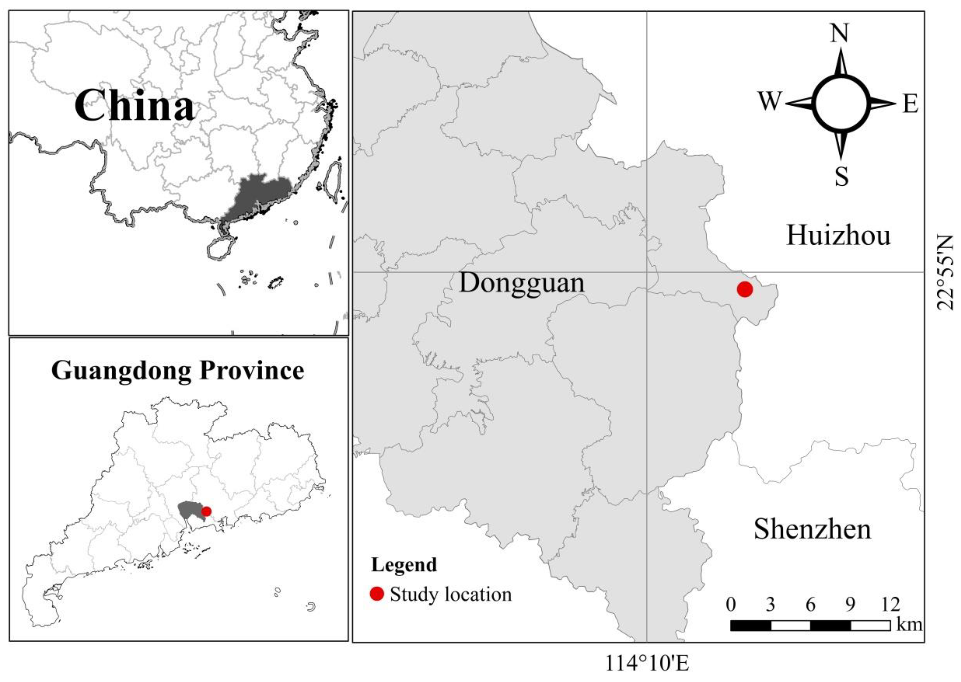
2.1. Study Sites

Our study sites were located in the Yinpingshan Nature Reserve (22°52′–22°56′ N, 114°05′–114°15′ E), along a slope on Mount Yinping, the core zone of the nature reserve. This area is in the southeastern part of Dongguan, South China’s Guangdong Province (Figure 1), and has a lower subtropical humid climate [17,18]. The mean annual temperature ranges from 21 °C to 22 °C, with the maximum mean temperature of 27.5 °C in July and the minimum mean temperature of 13.5 °C in January [17]. The mean annual precipitation is 1800 m, approximately 80% of which is concentrated from April to September [17]. Soil type is clay loamy latosol developed from granite. The peak of Mount Yinping is at an elevation of 898.2 m, the highest peak in the local area of Dongguan. Vegetation in the area is dominated by subtropical evergreen broadleaved forests [17,18].

2.2. Sampling Design and Data Collection

We established three 1 ha square plots on a forested slope of Mount Yinping in the nature reserve after topographic surveying with a total station (Nikon DTM-310, Nikon Geotecs Co., Ltd., Tokyo, Japan). We placed the plots in a relatively homogeneous evergreen broadleaved forest and separated them by at least 100 m in a vertical direction. Each plot was divided into 100 square quadrats or 10 × 10 m grid cells for plant and topographic data collection. The quadrats were numbered and marked by placing PVC (polyvinyl chloride) tubes at the 10 m corners. Elevation at each 10 m corner was recorded for calculation of slope and aspect of each quadrat [19]. Elevation for each quadrat was calculated by averaging the elevation values at its four corners [20].
We tallied all trees ≥ 1 cm diameter at breast height (DBH) in each quadrat. All censused individuals were identified to species and recorded with species name and DBH value measured to the nearest 0.1 cm. For exact DBH measurement, trees ≤ 5 cm DBH were measured with a dial caliper, while those > 5 cm DBH were measured with a diameter tape. Plant taxonomy and systematics followed Ye and Peng [21]. All the field data were entered in a spreadsheet to construct species-by-quadrat datasets for further calculations.

2.3. Statistical Analysis

We calculated species richness (number of species), total abundance (number of stems), the Shannon–Wiener diversity index, and Pielou’s evenness for each quadrat using the species-by-quadrat dataset. Shannon–Wiener diversity index and Pielou’s evenness were calculated with the following formula [22]:
H = P i l n P i
E = H / l n S
where H′ is the Shannon–Wiener diversity index, Pi is the relative abundance of the i-th species in proportion to the total abundance of species in a quadrat; and E is the Pielou’s evenness, S is the number of species in a quadrat.
Size diversity was represented by variability in basal area (BA), size diversity index, and evenness [15]. We defined the size diversity as the variability in basal areas across quadrats. The size diversity index and evenness were calculated following Su, Jia, Zhang and Chen [15], which are based on the Shannon–Wiener index formula and Pielou’s evenness, respectively.
D s i z e = P B A i l n P B A i
E s i z e = D s i z e / l n S
where Dsize is the size diversity index, PBAi is the relative basal area of the i-th species in proportion to the total basal area of species in a quadrat.
To test the effect of the inverse elevation-dependent warming on structural diversity of woody plant communities, we first grouped all tree individuals into three size classes, i.e., seedlings, saplings, and adults, as defined by DBH values using the following criteria [16]: seedlings, 1 cm ≤ DBH < 2.5 cm; saplings: 2.5 cm ≤ DBH < 12.5 cm; adults: DBH ≥ 12.5 cm. Therefore, we calculated the species diversity, size diversity, and evenness indices by four size groups, i.e., all sizes, seedlings, saplings, and adults, for each quadrat. We then used Kruskal–Wallis test, a nonparametric alternative to analysis of variance (ANOVA) that is appropriate for analyzing field ecology data [16], to test for significant differences in these diversity metrics across the three communities along an inverse elevational gradient.
We used the topographic data measured during plot establishment to calculate quadrat-based potential direct incident radiation (PDIR, MJ m−2 d−1) with nonparametric multiplicative regression (NPMR) [23], using the software HyperNiche: Nonparametric multiplicative habitat modeling, version 2.28 (MjM Software, Gleneden Beach, OR, USA).
We calculate an inverse elevation-dependent warming index for each quadrat using the following formula [10]:
Warming index = (Elevmax − Elevquadrat) m/100 m
where Elevmax is the elevation of the highest quadrat, while Elevquadrat is the elevation of a particular quadrat including the highest one. Therefore, the elevational difference of the highest quadrat, or hence the warming index, equals zero [10].
We performed principal component analysis (PCA) on the species-by-quadrat abundance dataset to reduce the dimensions to fewer orthogonal axes. PCA is a conventional ordination method that allows the analysis of datasets of non-independent variables, such as species composition data [24]. We extracted the scores or eigenvectors of the first two PCA axes and assessed the effects of warming on tree species composition by relating the axis scores to warming index and PDIR by axis overlays.
To evaluate the differences in species composition across communities of an inverse elevation gradient, we performed multi-response permutation procedures (MRPP). MRPP is a nonparametric multivariate method for testing the hypothesis of no difference between two or more groups of entities [25], such as plant communities and forest stands with compositional data. The output of MRPP includes an agreement statistic A, which describes within-group homogeneity, and the test statistic T, which describes the separation between the groups [25]. A p-value is calculated based on randomizations in MRPP [25].
To assess the contributions of some key species to the resemblance as well as separation of groups (communities), we plot the quadrat occurrence, species abundance, and total basal area of the shared species with all presence in the three communities. We also performed indicator species analysis (ISA) to identify species indicative of a community of a particular elevation. We calculated indicator values for each species in each community using Dufrêne and Legendre’s method [25], which combines information on the concentration of species abundance in a particular community and the faithfulness of occurrence of a species in that community [25]. An indicator value for a species in a particular community was expressed as a percentage. The highest indicator value of a species across communities was regarded as the overall indicator value of that species for a particular community [18,25]. The cut-off of the indicator value as a criterion for detecting indicator species for a particular group is usually arbitrary. An indicator value of 25 may, on average, correspond to a relative abundance of 50% and a relative frequency of 50%, because the indicator value is based on the product of relative abundance and relative frequency [25].
The calculation of diversity metrics, PCA ordination and axis overlays, MRPP, and ISA were carried out with PC-ORD: Multivariate analysis of ecological data, version 7 (MjM Software, Gleneden Beach, OR, USA). Descriptive statistics and Kruskal–Wallis tests were executed with Statistica version 8 (Statsoft, Inc. Tulsa, OK, USA).

3. Results

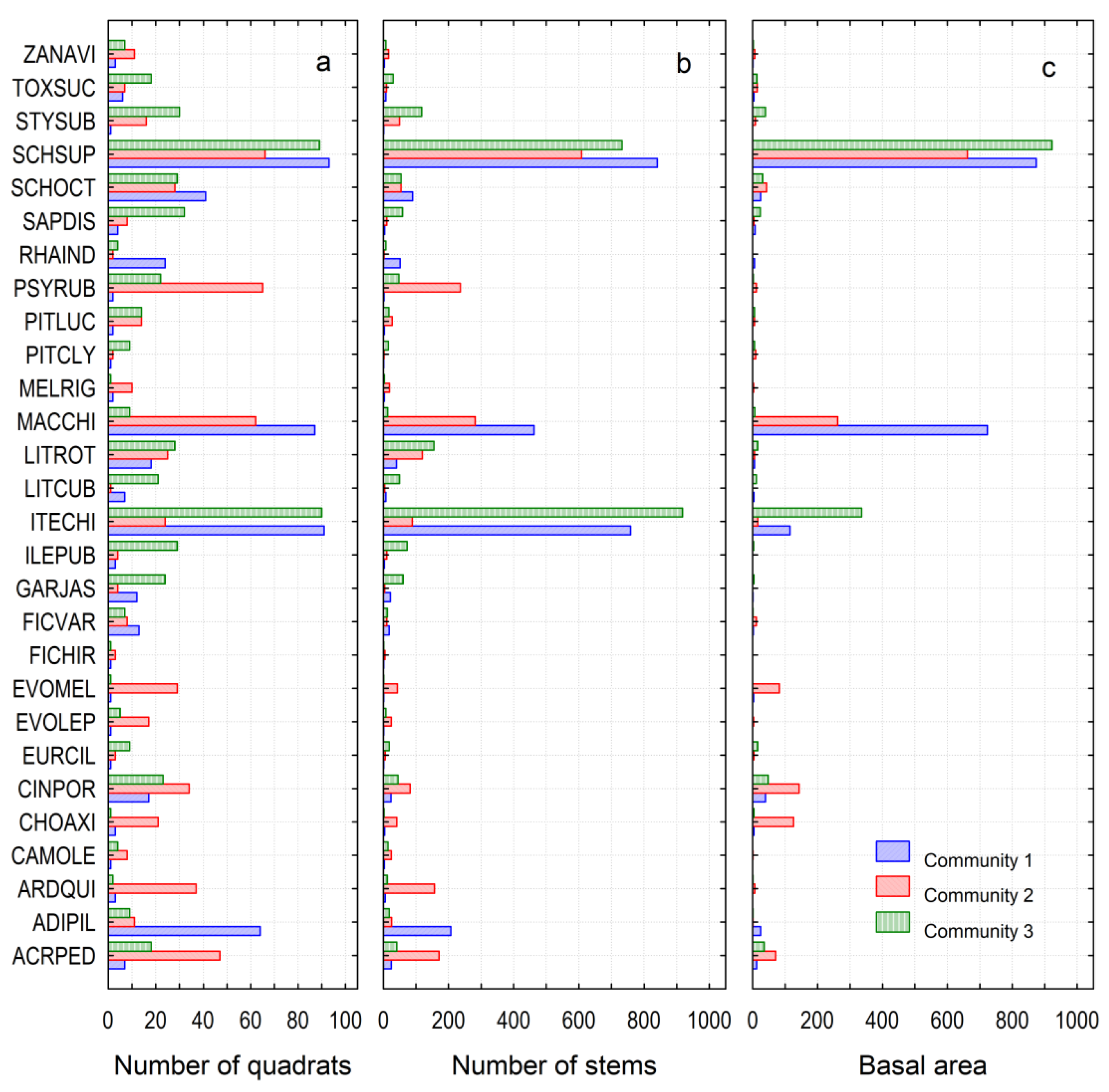
3.1. Community Structure

The three forest communities we investigated were relatively homogeneous in the way that they had similar dominant species (Table 1). The total number of taxa summed up from all the communities, or the γ-diversity, was 152 species from 105 genera and 54 families, representing 11,149 individual trees (Table 1). The total basal area in the aggregate for each community showed a general decreasing trend with decreasing elevation, which was consistent with the change in total abundance (Table 1). For the number of taxa, the community at the highest elevation is greater than the community at the lowest elevation; however, the biggest number of species, genera, and families were found in the community at the mid-elevation (Table 1).
Twenty-eight species were simultaneously shared by the three communities at different elevations (Figure 2). These species with all presence in the communities represented 7247 individual trees, approximately 2/3 of the total number of individuals found in the communities; however, they differed in quadrat occurrence, species abundance, and total basal area across communities (Figure 2). As shown in Figure 2a, the five most common species with an overall quadrat occurrence were Schima superba Gardner et Champ. (248), Itea chinensis Hook. et Arn. (205), Machilus chinensis (Benth.) Hemsl. (158), Schefflera octophylla (Lour.) Harms (98), and Psychotria rubra (Lour.) Poir. (89). Species varied in their distribution among the communities. Both Schima superba and Itea chinensis had approximately 90% quadrat frequency in Community 1 as well as in Community 3; however, Schima superba had 66% quadrat frequency (66 out of the 100 quadrats) in Community 2, whereas Itea chinensis had only 24% quadrat frequency in Community 2.
As shown in Figure 2b, the five most abundant species summed up from all three communities were Schima superba (2182 stems), Itea chinensis Hook. et Arn. (1765 stems), Machilus chinensis (756 stems), Litsea rotundifolia Hemsl. (314 stems), and Psychotria rubra (286 stems). Seventeen of the shared species had an abundance of less than 100 stems. The most abundant species, Schima superba, had 841 stems distributed in Community 1, 609 in Community 2, and 732 in Community 3, while other species were distributed in a more aggregated pattern. For example, the second most abundant species, Itea chinensis, had 758 stems distributed in Community 1 and 918 stems in Community 3, but only 89 stems in Community 2. Eight of the less abundant species had only one stem distributed in one of the communities and several to dozens of stems in two other communities (Figure 2b). The distribution of basal area of the species with all presence (Figure 2c) shared similar patterns with that of abundance (Figure 2b), as well as with quadrat occurrence among the communities, with only a few exceptions, such as for the two most abundant species, Schima superba and Itea chinensis.

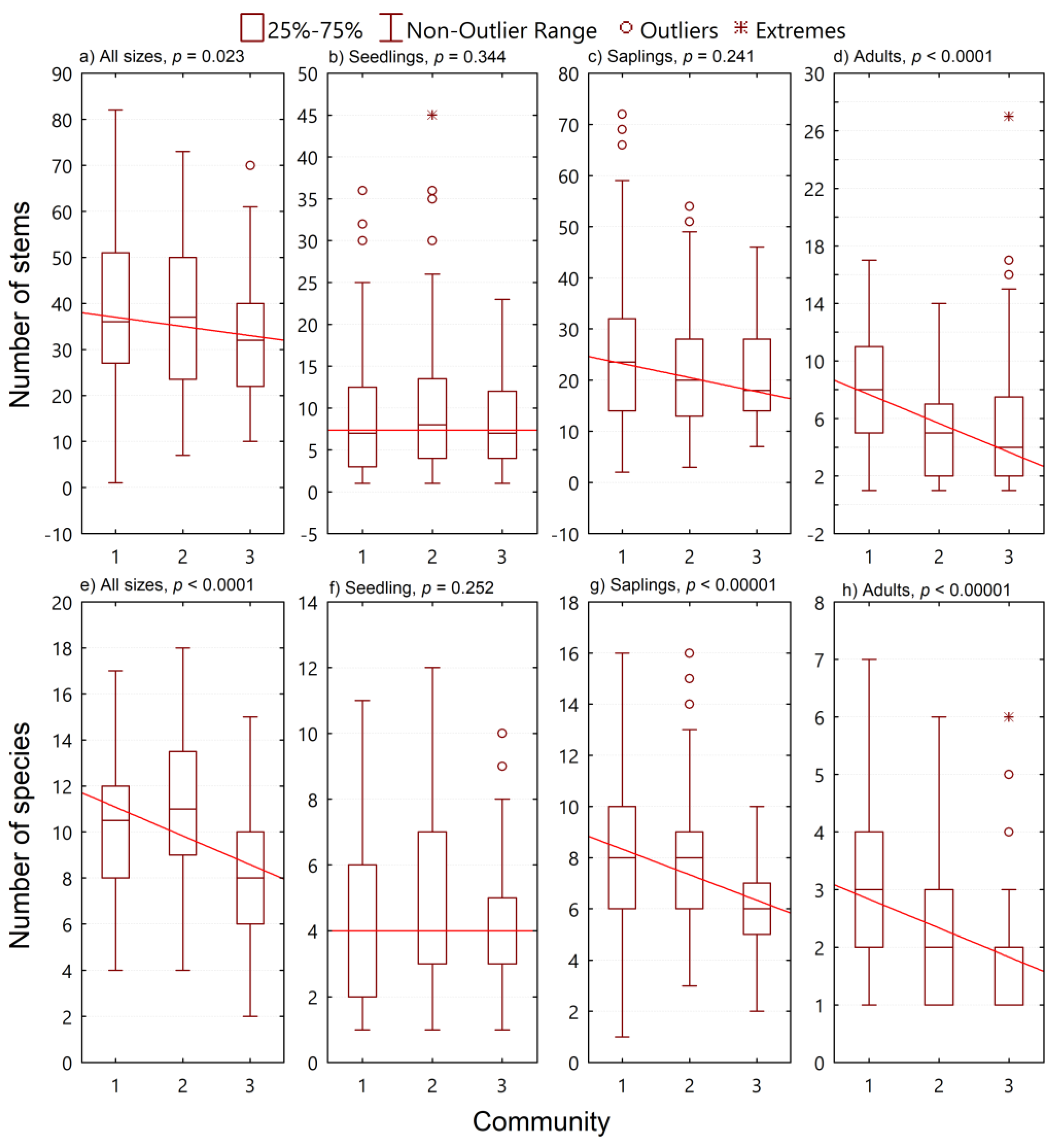
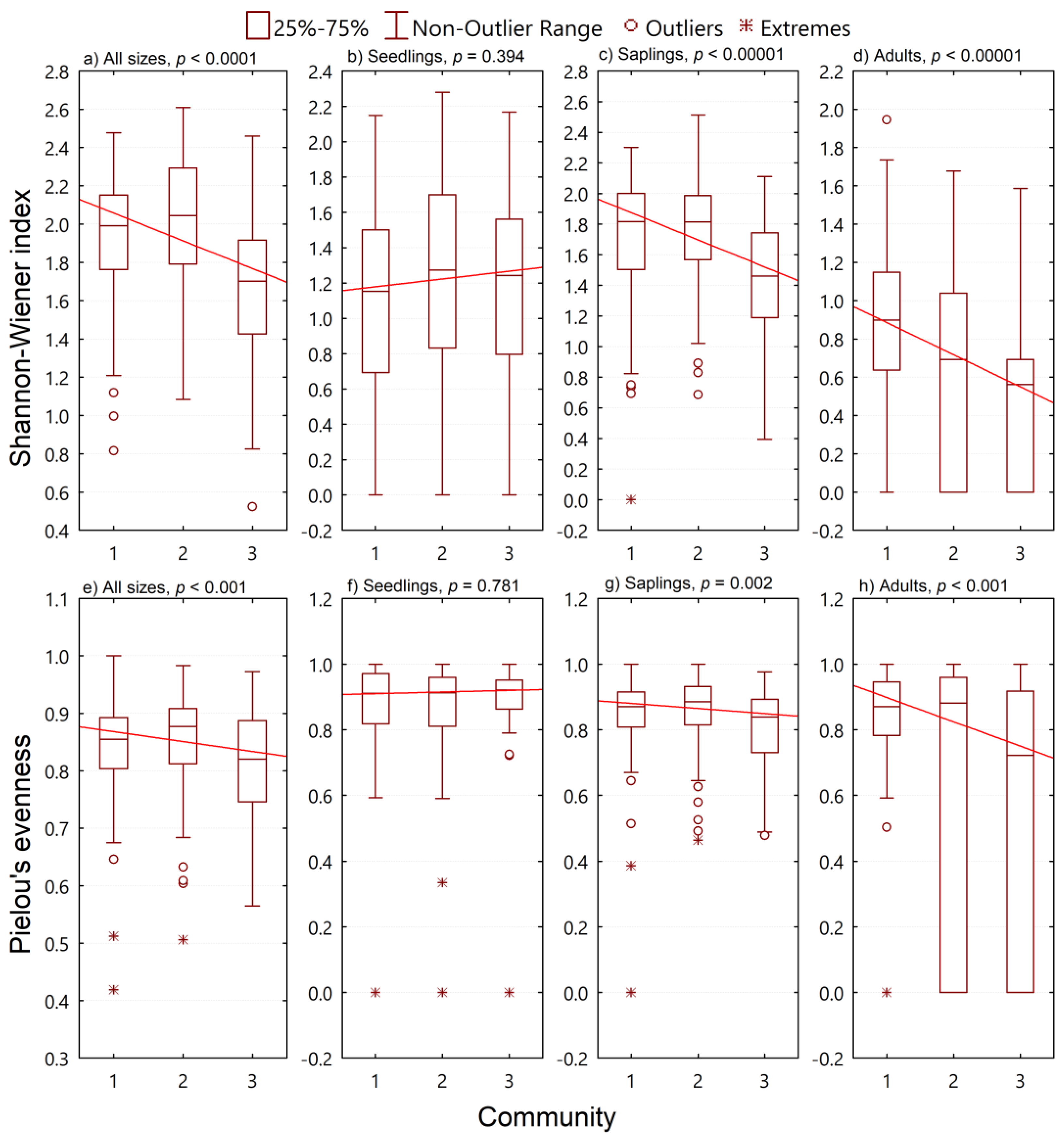
3.2. Species Diversity

Trees of different sizes responded differently to the inverse elevation-dependent warming gradient (Figure 3). For all sizes of trees (Figure 3a,e), as well as for adult trees (Figure 3d,h), quadrat-level species richness and total abundance significantly decreased across communities along an inverse elevation-dependent warming gradient; but for seedlings, no significant difference was found across a warming gradient (Figure 3b,f). The trends of change in both species richness and total abundance were consistent for trees of different sizes. For saplings, total abundance decreased with warming (Figure 3c), though this trend was not significant, while species richness significantly decreased with warming (Figure 3g). Within-community variability in both total abundance (Figure 3c) and species richness (Figure 3g) was the highest for saplings in Community 1 and lowest in Community 3, which was at the warmest elevation; but for adult trees, the warmest community (Community 3) exhibited broader min–max ranges and had more outliers and extreme values (Figure 3d,h).
The Shannon–Wiener diversity index and Pielou’s evenness (Figure 4) showed similar trends as compared with total abundance and species richness (Figure 3), except that the Shannon–Wiener index of seedlings exhibited an increasing trend with warming (Figure 4b), though not significant.

3.3. Size Diversity

Changes in size diversity across communities along a warming gradient (Figure 5) were different from those of species diversity (Figure 4). Changes in basal area across communities along a warming gradient showed a significant decreasing trend for trees of all sizes (Figure 5a, p < 0.00001) and adult trees (Figure 5d, p < 0.00001). A weak decreasing trend was found for saplings with marginal significance (Figure 5c, p = 0.065). Size diversity significantly decreased along a warming gradient for trees of all sizes (Figure 5e, p < 0.00001), saplings (Figure 5g, p < 0.0001), and adult trees (Figure 5h, p < 0.0001). No significant difference was found in the basal area (Figure 5b, p = 0.313) and size diversity index (Figure 5f, p = 0.176) for seedlings across communities. Changes in the basal area (Figure 5a–d) and size diversity index (Figure 5e–h) were similar to those in total abundance and species richness (Figure 3), respectively, indicating that the basal area was determined more by total abundance than by species richness and size diversity was determined more by species richness than by total abundance.
No significant difference was found in the size diversity-based evenness for seedlings, saplings, and trees of all sizes across communities, but for adult trees, the evenness significantly decreased across communities along a warming gradient (Figure 5m, p < 0.00001).

3.4. Species Composition

Multi-response permutation procedures (MRPP) indicated that the species composition of the communities at different elevations extremely differed by overall comparison as well as by pairwise comparison (Table 2). The species composition of Community 1 vs. Community 2 (MRPP, A = 0.10) was more homogeneous than either Community 1 vs. Community 3 (MRPP, A = 0.08) or Community 2 vs. Community 3 (MRPP, A = 0.09). The between-group difference was greater for Community 1 vs. Community 2, rather than for Community 1 vs. Community 3, or for Community 2 vs. Community 3.
Principal component analysis (PCA) well separated the three communities by the ordination of sample units in species space (Figure 6 and Figure 7). Two warming-related variables, warming index and potential direct incident radiation (PDIR), were significantly correlated with the first two principal components from PCA. As shown in Figure 6 and Figure 7, the warming index was negatively correlated with PCA axis 1 (Figure 6; r = −0.659, p = 0.0001) and Axis 2 (Figure 6; r = −0.359, p = 0.001), while PDIR was positively correlated with PCA axis 1 (Figure 7; r = 0.390, p = 0.001) and negatively correlated with PCA axis 2 (Figure 7; r = −0.338, p = 0.001).
The inverse elevation-dependent warming index was stronger than the aspect-related PDIR in their relationships with the first two PCA ordination axes (Figure 6 and Figure 7). The warming index also had greater strength in separating the communities than PDIR (Figure 6 and Figure 7).

3.5. Indicator Species

Twenty-two tree species were detected as bio-indicators of a particular community with a significant indicator value ≥ 25 (Table 3). These indicator species contributed to the separation of the communities. Nine out of these indicator species were found with all presence in the three communities (Figure 2 and Table 3). These were Acronychia pedunculata (L.) Miq., Adina pilulifera (Lam.) Franch. ex Drake, Ardisia quinquegona Blume, Evodia meliaefolia Benth., Itea chinensis Hook. et Arn., Machilus chinensis (Benth.) Hemsl., Psychotria rubra (Lour.) Poir., Sapium discolor (Champ.) Muell.-Arg., and Schima superba Gardner et Champ. These species only had low to medium indicator values (Table 3). The number of indicator species that separated a community from others with a significant indicator value was the highest for Community 2 (10 species), lowest for Community 3 (3 species), and medium for Community 1 (9 species), practically a decreasing trend along a warming gradient.
The species with the highest indicator value (IV = 77.0) for indicating Community 1, Rhodoleia championii, had a low indicator value averaged across the three communities by randomization (Table 3). By contrast, Schima superba had an indicator value of 35.8 for indicating Community 1, but it had the highest mean indicator value (IV = 30.6) for all the communities from randomization (Table 3). This result suggested that Schima superba was not uniquely indicative of a particular community. Although Schima superba was the most abundant species, its relative abundance and relative frequency in Community 1 as calculated among the three communities was not as high as other species with less abundance but in aggregated distribution, such as Adina pilulifera, Machilus chinensis, and Psychotria rubra.

4. Discussion

One of the most important spatial patterns that attracted ecologists and forest managers is the elevational or altitudinal pattern of plant communities [26,27,28,29]. In a broad-range elevational gradient, structural diversity is controlled predominantly by the coupling of water and heat [30,31], thus the changes in diversity patterns are similar to those in latitudinal patterns. In contrast, in a short-to-medium-range elevational gradient, changes in diversity patterns will be affected predominantly by temperature because of similar water availability from rainfalls. A small change in temperature due to the temperature lapse rate in mountain areas will exert an enormous influence on structural diversity [15,31,32].
Structural diversity is mainly composed of three components, i.e., spatial distribution, species diversity, and tree size diversity [15,33]. Changes in structural diversity are often affected by a variety of factors, including climate change [34,35], land use history [36], habitat heterogeneity [37], and inter- and intraspecific competitions [38,39]. Compared with other indicators, tree size is easy to measure using forestry tools [15,40]. Several biodiversity indices have been used in previous studies to evaluate the response of diversity to elevational gradients, however, the richness- or abundance-based diversity indices may not be so sensitive in response to warming as tree size-based diversity indices [16]. For species diversity, the most common indices are the Shannon–Wiener index, Simpson index, and Pielou’s evenness [40,41]. The Shannon–Wiener index reflects the species richness and evenness in a community, which is estimated by measuring the uncertainty of the category to which the randomly selected individuals belong, while the Simpson index represents the likelihood that two randomly chosen individuals in a community will be different species, and Pielou’s evenness index can reflect the uniformity of the number of individuals in the community [42]. However, traditional diversity indices cannot fully reflect the structural diversity of a community, because the diversity of a forest stand means a wide range of changes in tree species, size, and age class [16,40]. Therefore, an extension of the well-known Shannon–Wiener diversity index with DBH or basal area to diversify the diversity structure is more reasonable. This new index based on size structure not only has a similar diversity calculation method to the Shannon–Wiener index but also does not need to divide the diameter and basal area data into different classes. As shown in this study, using the size data to calculate the Shannon–Wiener index will undoubtedly provide a new indicator for the relationship between diversity and elevational gradient.
Previous reports have shown that patterns of species diversity along an elevational gradient varied with studies. Species diversity may decrease or increase [11,12,13], or it will exhibit a unimodal pattern or just unrelated [43] with elevation. These patterns might be site-specific so more studies should be carried out for adequate information to reach a sound conclusion, especially when these studies are taken into account the relationships with climate change. A review report by Chinese scholars documented various patterns of species diversity along an elevational gradient, with the prevailing conclusion that species diversity decreases with the increase in elevation [43]. Obviously, the decrease in species diversity is reasonable with a broad-scale elevation increase. Vegetation changes with a broad-scale elevation increase, such that the species diversity of scrublands, coniferous forests, or mountaintop dwarf forests that often occur at high elevations is lower than that of evergreen broadleaved forests at low elevations. In contrast, our results are completely different, that is, species diversity increases with elevation, or in other words, species diversity decreases along the inverse elevational warming gradient. This might be due to the fact that our study specifically examined the change in structural diversity of broadleaved forest communities along a short-range elevational change. It also indicated that only a short-range elevation-dependent warming gradient can make appreciable changes in the structural diversity of the subtropical broadleaved forests.
Although we set up a short-range inverse elevational warming gradient using three evergreen broadleaved forest plots at different elevations and tested the effect of warming on forest biodiversity, a broad spatial gradient, as well as a temporal gradient in combination, should be considered for study in the subtropical area. A broad spatial gradient combined with varied forest types may show differential patterns of changes in structural diversity, which calls for comparative studies. Moreover, whether the global warming trend and extreme climatic events, such as massive floods and cyclones that frequently occur in this area, will alter the response of forest structural diversity to warming should also be explored.

5. Conclusions

Our results demonstrated that a short-range elevational gradient was adequate to separate the communities in a homogeneous broadleaved evergreen forest in species composition and structural diversity. Patterns of species richness, total abundance, species diversity, and tree size diversity along an inverse elevational gradient varied in size classes and were scale-dependent. The first two principal components were negatively correlated with the warming index, indicating that warming destabilized species composition and community structure. The community at a higher elevation had more indicator species that were unique in separating the community from others. Our study suggests that warming is the major driver of changes in structural diversity and species composition of woody plant communities in a subtropical broadleaved forest.

Author Contributions

Conceptualization, Y.S. and W.Z.; methodology, Y.S. and X.G.; formal analysis, Y.S.; investigation, Y.S., X.G., W.Z., G.W. and F.H.; data curation, Y.S., G.W. and F.H.; writing—original draft preparation, Y.S.; writing—review and editing, Y.S. and W.Z.; funding acquisition, W.Z. All authors have read and agreed to the published version of the manuscript.

Funding

This research was supported jointly by the Forestry Sci-Tech Innovation Program of Guangdong Province, China (2021KJCX003), the Sci-Tech Innovation Platform Operation Fund of the National Forestry and Grassland Administration (2021132084; 2021132085), and the Sci-Tech Innovation Platform Project of Guangdong Province, China (2021-KYXM-09).

Data Availability Statement

The data presented in this study are available on request from the corresponding author.

Acknowledgments

We thank the staff of the Yinpingshan Nature Reserve of Dongguan, Guangdong Province, China, for logistic support during the field investigation.

Conflicts of Interest

The authors declare no conflicts of interest.

References

  1. Haider, S.; Kueffer, C.; Bruelheide, H.; Seipel, T.; Alexander, J.M.; Rew, L.J.; Arévalo, J.R.; Cavieres, L.A.; McDougall, K.L.; Milbau, A. Mountain roads and non-native species modify elevational patterns of plant diversity. Global Ecol. Biogeogr. 2018, 27, 667–678. [Google Scholar] [CrossRef]
  2. Karger, D.N.; Kluge, J.; Krömer, T.; Hemp, A.; Lehnert, M.; Kessler, M. The effect of area on local and regional elevational patterns of species richness. J. Biogeogr. 2011, 38, 1177–1185. [Google Scholar] [CrossRef]
  3. Toivonen, J.M.; Gonzales-Inca, C.A.; Bader, M.Y.; Ruokolainen, K.; Kessler, M. Elevational shifts in the topographic position of Polylepis forest stands in the Andes of southern Peru. Forests 2018, 9, 7. [Google Scholar] [CrossRef]
  4. Haq, S.M.; Calixto, E.S.; Rashid, I.; Srivastava, G.; Khuroo, A.A. Tree diversity, distribution and regeneration in major forest types along an extensive elevational gradient in Indian Himalaya: Implications for sustainable forest management. Forest Ecol. Manag. 2022, 506, 119968. [Google Scholar] [CrossRef]
  5. Pepin, N.; Bradley, R.S.; Diaz, H.; Baraër, M.; Caceres, E.; Forsythe, N.; Fowler, H.; Greenwood, G.; Hashmi, M.; Liu, X. Elevation-dependent warming in mountain regions of the world. Nat. Clim. Change 2015, 5, 424–430. [Google Scholar]
  6. Rangwala, I.; Miller, J.R. Climate change in mountains: A review of elevation-dependent warming and its possible causes. Clim. Change 2012, 114, 527–547. [Google Scholar] [CrossRef]
  7. Tudoroiu, M.; Eccel, E.; Gioli, B.; Gianelle, D.; Schume, H.; Genesio, L.; Miglietta, F. Negative elevation-dependent warming trend in the Eastern Alps. Environ. Res. Lett. 2016, 11, 044021. [Google Scholar] [CrossRef]
  8. Thayyen, R.J.; Dimri, A.P. Modeling slope environmental lapse rate (SELR) of temperature in the monsoon glacio-hydrological regime of the Himalaya. Cryosphere Discuss. 2016, 1–35. [Google Scholar] [CrossRef]
  9. Singh, P.; Bengtsson, L. Hydrological sensitivity of a large Himalayan basin to climate change. Hydrol. Process 2004, 18, 2363–2385. [Google Scholar] [CrossRef]
  10. Su, Y.; Wu, Z.; Xie, P.; Zhang, L.; Chen, H. Warming effects on topsoil organic carbon and C: N: P stoichiometry in a subtropical forested landscape. Forests 2020, 11, 66. [Google Scholar] [CrossRef]
  11. Lee, C.; Chun, J.; Cho, H. Elevational patterns and determinants of plant diversity in the Baekdudaegan Mountains, South Korea: Species vs. functional diversity. Chin. Sci. Bull. 2013, 58, 3747–3759. [Google Scholar] [CrossRef]
  12. Kromer, T.; Acebey, A.; Kluge, J.; Kessler, M. Effects of altitude and climate in determining elevational plant species richness patterns: A case study from Los Tuxtlas, Mexico. Flora 2013, 208, 197–210. [Google Scholar] [CrossRef]
  13. Oishi, Y. Factors that shape the elevational patterns of plant diversity in the Yatsugatake Mountains, Japan. Ecol. Evol. 2021, 11, 4887–4897. [Google Scholar] [CrossRef]
  14. Wu, G.P.; Su, Y.G.; Wang, J.J.; Lin, S.N.; Huang, Z.Y.; Huang, G. Elevational patterns of microbial carbon use efficiency in a subtropical mountain forest. Biol. Fert. Soils 2023, 60, 5–15. [Google Scholar] [CrossRef]
  15. Su, Y.; Jia, X.; Zhang, L.; Chen, H. Size-dependent associations of woody plant structural diversity with soil C:N:P stoichiometry in a subtropical forest. Front. Environ. Sci. 2022, 10, 990387. [Google Scholar] [CrossRef]
  16. He, S.; Zhong, Y.; Sun, Y.; Su, Z.; Jia, X.; Hu, Y.; Zhou, Q. Topography-associated thermal gradient predicts warming effects on woody plant structural diversity in a subtropical forest. Sci. Rep. 2017, 7, 40387. [Google Scholar] [CrossRef]
  17. Su, Y.; Zhang, Y.; Jia, X.; Xue, Y. Application of several diversity indexes in forest community analysis. Ecol. Sci. 2017, 36, 132–138. [Google Scholar]
  18. Zhou, Y.; Su, Y.; Zhong, Y.; Xie, P.; Xu, M.; Su, Z. Community attributes predict the relationship between habitat invasibility and land use types in an agricultural and forest landscape. Forests 2019, 10, 867. [Google Scholar] [CrossRef]
  19. Lai, J.; Mi, X.; Ren, H.; Ma, K.J.J.o.V.S. Species-habitat associations change in a subtropical forest of China. J. Veg. Sci. 2009, 20, 415–423. [Google Scholar] [CrossRef]
  20. Condit, R. Tropical Forest Census Plots: Methods and Results from Barro Colorado Island, Panama and a Comparison with Other Plots; Springer: Berlin/Heidelberg, Germany, 1998. [Google Scholar]
  21. Ye, H.G.; Peng, S.L. Plant Diversity Inventory of Guangdong; Guangdong World Publishing Corporation: Guangzhou, China, 2006. [Google Scholar]
  22. Magurran, A.E.; McGill, B.J. Biological Diversity: Frontiers in Measurement and Assessment; Oxford University Press: New York, NY, USA, 2011. [Google Scholar]
  23. McCune, B. Improved estimates of incident radiation and heat load using non-parametric regression against topographic variables. J. Veg. Sci. 2007, 18, 751–754. [Google Scholar]
  24. Santos, R.M.; Oliveira, A.T.; Eisenlohr, P.V.; Queiroz, L.P.; Cardoso, D.B.O.S.; Rodal, M.J.N. Identity and relationships of the Arboreal Caatinga among other floristic units of seasonally dry tropical forests (SDTFs) of north-eastern and Central Brazil. Ecol. Evol. 2012, 2, 409–428. [Google Scholar] [CrossRef]
  25. McCune, B.; Grace, J.B.; Urban, D.L. Analysis of Ecological Communities; MjM Software Design: Gleneden Beach, OR, USA, 2002. [Google Scholar]
  26. Lee, C.B.; Chun, J.H. Patterns and determinants of plant richness by elevation in a mountain ecosystem in South Korea: Area, mid-domain effect, climate and productivity. J. For. Res. 2015, 26, 905–917. [Google Scholar] [CrossRef]
  27. Xu, X.; Zhang, H.Y.; Zhang, D.J.; Tian, W.; Huang, H.; Ma, A. Altitudinal patterns of plant species richness in the Honghe region of China. Pak. J. Bot. 2017, 49, 1039–1048. [Google Scholar]
  28. Gheyret, G.; Guo, Y.P.; Fang, J.Y.; Tang, Z.Y. Latitudinal and elevational patterns of phylogenetic structure in forest communities in China’s mountains. Sci. China Life Sci. 2020, 63, 1895–1904. [Google Scholar] [CrossRef]
  29. Zhao, M.F.; Wang, Y.H.; Xue, F.; Zuo, W.Y.; Xing, K.X.; Wang, G.Y.; Kang, M.Y.; Jiang, Y. Elevational patterns and ecological determinants of mean family age of angiosperm assemblages in temperate forests within Mount Taibai, China. J. Plant Ecol. 2018, 11, 919–927. [Google Scholar] [CrossRef]
  30. Ali, A.; Lin, S.L.; He, J.K.; Kong, F.M.; Yu, J.H.; Jiang, H.S. Climatic water availability is the main limiting factor of biotic attributes across large-scale elevational gradients in tropical forests. Sci. Total Environ. 2019, 647, 1211–1221. [Google Scholar] [CrossRef]
  31. Randin, C.F.; Paulsen, J.; Vitasse, Y.; Kollas, C.; Wohlgemuth, T.; Zimmermann, N.E.; Korner, C. Do the elevational limits of deciduous tree species match their thermal latitudinal limits? Global Ecol. Biogeogr. 2013, 22, 913–923. [Google Scholar] [CrossRef]
  32. Halbritter, A.H.; Alexander, J.M.; Edwards, P.J.; Billeter, R. How comparable are species distributions along elevational and latitudinal climate gradients? Global Ecol. Biogeogr. 2013, 22, 1228–1237. [Google Scholar] [CrossRef]
  33. Zlatanov, T.; Schleppi, P.; Velichkov, I.; Hinkov, G.; Georgieva, M.; Eggertsson, O.; Zlatanova, M.; Vacik, H. Structural diversity of abandoned chestnut (Castanea sativa Mill.) dominated forests: Implications for forest management. Forest Ecol. Manag. 2013, 291, 326–335. [Google Scholar] [CrossRef]
  34. Xu, M.H.; Zhang, S.X.; Wen, J.; Yang, X.Y. Multiscale spatial patterns of species diversity and biomass together with their correlations along geographical gradients in subalpine meadows. PLoS ONE 2019, 14, e0211560. [Google Scholar] [CrossRef]
  35. Maharjan, S.K.; Sterck, F.J.; Raes, N.; Poorter, L. Temperature and soils predict the distribution of plant species along the Himalayan elevational gradient. J. Trop. Ecol. 2022, 38, 58–70. [Google Scholar] [CrossRef]
  36. Monge-Gonzalez, M.L.; Craven, D.; Kromer, T.; Castillo-Campos, G.; Hernandez-Sanchez, A.; Guzman-Jacob, V.; Guerrero-Ramirez, N.; Kreft, H. Response of tree diversity and community composition to forest use intensity along a tropical elevational gradient. Appl. Veg. Sci. 2020, 23, 69–79. [Google Scholar] [CrossRef]
  37. Ramos, C.S.; Picca, P.; Pocco, M.E.; Filloy, J. Disentangling the role of environment in cross-taxon congruence of species richness along elevational gradients. Sci. Rep. 2021, 11, 4711. [Google Scholar] [CrossRef]
  38. Knight, K.S.; Oleksyn, J.; Jagodzinski, A.M.; Reich, P.B.; Kasprowicz, M. Overstorey tree species regulate colonization by native and exotic plants: A source of positive relationships between understorey diversity and invasibility. Divers. Distrib. 2008, 14, 666–675. [Google Scholar] [CrossRef]
  39. Urza, A.K.; Weisberg, P.J.; Chambers, J.C.; Sullivan, B.W. Shrub facilitation of tree establishment varies with ontogenetic stage across environmental gradients. New Phytol. 2019, 223, 1795–1808. [Google Scholar] [CrossRef]
  40. Zhong, Y.; Sun, Y.; Xu, M.; Zhang, Y.; Wang, Y.; Su, Z. Spatially destabilising effect of woody plant diversity on forest productivity in a subtropical mountain forest. Sci. Rep. 2017, 7, 9551. [Google Scholar] [CrossRef]
  41. Sharma, C.M.; Mishra, A.K.; Tiwari, O.P.; Krishan, R.; Rana, Y.S. Regeneration patterns of tree species along an elevational gradient in the Garhwal Himalaya. Mt. Res. Dev. 2018, 38, 211–219. [Google Scholar] [CrossRef]
  42. Ke, X.; Su, Z.; Hu, Y.; Zhou, Y.; Xu, M. Measuring species diversity in a subtropical forest across a tree size gradient: A comparison of diversity indices. Pak. J. Bot. 2017, 49, 1373–1379. [Google Scholar]
  43. He, J.; Chen, W. A review of gradient changes in species diversity of land plant communities. Acta Ecol. Sin. 1997, 17, 91–99. [Google Scholar]
Figure 1. Location of the study sites in Dongguan, Guangdong Province, China.
Forests 15 01051 g001
Figure 2. Quadrat occurrence (a), species abundance (b), and total basal area (dm2) (c) of the twenty-eight shared species with all presence in the communities along an inverse elevational gradient. The community codes represent the average elevations of a community: 1, 576.9 m; 2, 433.2 m; and 3, 239.5 m. Species codes: ACRPED, Acronychia pedunculata (L.) Miq.; ADIPIL, Adina pilulifera (Lam.) Franch. ex Drake; ARDQUI, Ardisia quinquegona Blume; CAMOLE, Camellia oleifera Abel; CHOAXI, Choerospondias axillaris (Roxb.) Burtt et Hill; CINPOR, Cinnamomum porrectum (Roxb.) Kosterm.; EURCIL, Eurya ciliata Merr.; EVOLEP, Evodia lepta Merr.; EVOMEL, Evodia meliaefolia Benth.; FICHIR, Ficus hirta Vahl; FICVAR, Ficus variolosa Lindl. ex Benth.; GARJAS, Gardenia jasminoides Ellis; ILEPUB, Ilex pubescens Hook. et Arn.; ITECHI, Itea chinensis Hook. et Arn.; LITCUB, Litsea cubeba (Lour.) Pers.; LITROT, Litsea rotundifolia Hemsl.; MACCHI, Machilus chinensis (Benth.) Hemsl.; MELRIG, Meliosma rigida Sieb. et Zucc.; PITCLY, Pithecellobium clypearia Benth.; PITLUC, Pithecellobium lucidum Benth.; PSYRUB, Psychotria rubra (Lour.) Poir.; RHAIND, Rhaphiolepis indica Lindl.; SAPDIS, Sapium discolor (Champ.) Muell.-Arg.; SCHOCT, Schefflera octophylla (Lour.) Harms; SCHSUP, Schima superba Gardner et Champ.; STYSUB, Styrax suberifolia Hook. et Arn.; TOXSUC, Toxicodendron succedaneum (L.) Kuntze; ZANAVI, Zanthoxylum avicennae (Lam.) DC.
Forests 15 01051 g002
Figure 3. Boxplots showing changes in total abundance (ad) and species richness (eh) across communities at different elevations. The community codes represent the average elevations of a community: 1, 576.9 m; 2, 433.2 m; and 3, 239.5 m.
Forests 15 01051 g003
Figure 4. Boxplots showing changes in the Shannon–Wiener diversity index (ad) and Pielou’s evenness (eh) across communities at different elevations. The community codes represent the average elevations of a community: 1, 576.9 m; 2, 433.2 m; and 3, 239.5 m.
Forests 15 01051 g004
Figure 5. Boxplots showing changes in basal area (dm2, (ad)), size diversity index (eh), and evenness (im) across communities at different elevations. The community codes represent the average elevations of a community: 1, 576.9 m; 2, 433.2 m; and 3, 239.5 m.
Forests 15 01051 g005
Figure 6. PCA ordination diagram showing changes in sample units with overlays of warming index on the first two axes.
Forests 15 01051 g006
Figure 7. PCA ordination diagram showing changes in sample units with overlays of potential direct incident radiation (PDIR) on the first two axes.
Forests 15 01051 g007
Table 1. Summary of community characteristics for the three 1 ha plots at different elevations.
AttributeCommunityγ-Diversity
123
Mean elevation (m)576.9433.2239.5
Number of stems41773683328911,149
Number of species858966152
Number of genera597253105
Number of families36432954
Total basal area (m2/ha)30.38921.18324.537
Average basal area (cm2/tree)72.7557.5274.60
Dominant speciesSchima superba,
Itea chinensis
Machilus chinensis
Schima superba
Aporosa dioica
Machilus chinensis
Itea chinensis
Schima superba
Castanopsis fissa
Table 2. Multi-response permutation procedures (MRPP) for the species composition across communities. Explanation of the MRPP statistics: A is a measure of effect size and represents the within-group homogeneity; T is a statistic describing the separation between the groups; p is the p-value for significance test of homogeneity using randomization. Community 1, Community 2, and Community 3 are each represented by 1 ha plot at 576.9 m, 433.2 m, and 239.5 m a.s.l., respectively.
Communities ComparedTAp
Overall comparison−119.00.12<10−7
Pairwise comparison
Community 1 vs. Community 2−91.470.10<10−7
Community 1 vs. Community 3−72.640.08<10−7
Community 2 vs. Community 3−80.150.09<10−7
Table 3. Woody plant species indicative of a particular community with a significant indicator value ≥ 25.
Indicator SpeciesIndicated
Community
Observed Indicator ValueIndicator Value from Randomized Groupsp-Value
MeanSD
Adina pilulifera (Lam.) Franch. ex Drake15312.41.910.001
Dendropanax proteus (Harmp.) Benth.1447.51.670.001
Diospyros morrisiana Hance1599.31.720.001
Enkianthus quinqueflorus Lour.1295.41.360.001
Machilus chinensis (Benth.) Hemsl.153.221.12.240.001
Rapanea neriifolia (S. et Z.) Mez1559.11.990.001
Rhodoleia championii Benth.17711.62.00.001
Schima superba Gardner et Champ.135.830.62.010.006
Symplocos crassilimba Merr.1356.31.50.001
Acronychia pedunculata (L.) Miq.234.110.91.940.001
Adenanthera pavonina L.253.68.91.720.001
Aporosa dioica (Roxb.) Muell.-Arg.258.315.22.150.001
Ardisia quinquegona Blume233.27.31.790.001
Evodia meliaefolia Benth.227.75.51.420.001
Psychotria rubra (Lour.) Poir.253.613.22.070.001
Scolopia saeva (Hance) Hance23361.390.001
Syzygium jambos (L.) Alston2356.21.560.001
Syzygium rehderianum Merr. et Perry2619.41.690.001
Viburnum odoratissimum Ker.2295.31.370.001
Castanopsis fissa Rehder and E.H.Wilson3467.71.690.001
Itea chinensis Hook. et Arn.346.826.12.140.001
Sapium discolor (Champ.) Muell.-Arg.325.97.31.550.001
Disclaimer/Publisher’s Note: The statements, opinions and data contained in all publications are solely those of the individual author(s) and contributor(s) and not of MDPI and/or the editor(s). MDPI and/or the editor(s) disclaim responsibility for any injury to people or property resulting from any ideas, methods, instructions or products referred to in the content.

