Construction of Compatible Volume Model for Populus in Beijing, China

Abstract

The accurate assessment of tree volume is crucial for developing forest management plans, and this can be achieved using tree volume models. In this study, data on individual trees were collected and calculated, including the diameter at breast height (D), ground diameter (DG), tree height (H), and tree volume (V). A total of 400 Populus × tomentosa Carrière, 400 Populus tomentosa Carr, and 400 Populus × canadensis Moench trees were sampled. Two compatible volume model systems were established using corresponding methods. The models consisted of the following five types: V-DH, V-D, V-DG, H-D, and DG-D. In our calculations, before the horizontal line was the dependent variable, and behind the horizontal line was the independent variable. Variations in preferences for the H-D models were observed among the tree species, with the logistic function proving the most suitable for Populus × tomentosa Carrière, Chapman–Richard function for Populus tomentosa Carr, and power function for Populus × canadensis Moench. Among the three volume models, the V-DH model exhibited a superior performance, with its R² values ranging from 0.965 to 0.984 and mean estimated error (MPE) values ranging from 1.26% to 1.78%. Following this was the V-D model, with R² values between 0.9359 and 0.9704 and MPE values between 1.71% and 2.46%. The V-DG model ranked third, with R² values ranging from 0.8746 to 0.9501 and MPE values ranging from 2.33% to 3.16%. In the H-D model, the R² and MPE values ranged from 0.4998 to 0.7851 and from 1.31% to 1.45%, respectively. For the DG-D model, the R² values ranged from 0.9563 to 0.9868 and the MPE values ranged from 0.47% to 0.68%. Comparing both compatible methods, the nonlinear seemingly uncorrelated regression (NSUR) was more effective. The three volume models demonstrated high levels of accuracy and compatibility, providing a reliable scientific foundation for forest management and the formulation of harvesting plans in Beijing, with significant practical implications.

1. Introduction

Populus L. is, globally, the most widely distributed and adaptable tree species, with rapid growth and significant economic value [1]. Accurately assessing the wood resources of this species in Beijing is of considerable practical importance and will aid forest managers in timber valuation and the allocation of forest harvesting areas [2].

Undoubtedly, the most reliable approach for acquiring tree volume data is the harvesting of all trees in a forest. However, this method is characterized by its destructiveness, time intensiveness, and high cost, rendering it feasible only on a limited scale [3]. With advancements in modern science and technology, foresters have turned to precision measurement instruments for forest surveys. Certain studies have applied airborne laser radar to conduct large-scale measurements of vegetation structures, realizing accurate estimations of tree volumes, biomass, and carbon storage [4]. Nevertheless, precision equipment is expensive and involves technical complexities, limiting its widespread application in forestry investigations. Other studies have employed total station and electronic theodolite for measuring tree heights, volumes, and other basic tree factors (e.g., diameters at breast height) [5,6,7]. Total station equipment is costly, lacks portability, and faces challenges in measuring within complex stands, whereas electronic theodolites offer a comparatively lower cost, lighter weight, ease of transport, and operational simplicity.

Volume models offer a nondestructive method for estimating tree volume [8]. National-scale volume models have limited accuracy and applicability. Due to the variability in ecological conditions across large geographic areas, the predictive accuracy of these models decreases when they are applied to smaller scales [9,10,11]. For example, Case and Hall (2008) compared volume models at local, regional, and national scales for 10 tree species in central and western Canada [11]. As the generality of the model increased, the estimation error for local areas increased. In China, by the late 1970s, only three poplar volume tables specific to Populus davidiana Dode in the northeast, north, and northwest regions were enforced. A locally developed volume model offers a more precise estimate [12]. Therefore, establishing a poplar volume model for the Beijing area appears to be more feasible.

Most studies have utilized multivariate statistical methods to construct volume models, which are known for their clarity in expression. Conversely, some studies have employed machine learning techniques such as artificial neural networks, support vector machines, and random forests for volume modeling [13,14,15]. Compared with machine learning, a multivariate statistical model cannot easily fit large-scale data containing noise [16]. Although machine learning adeptly handles complex nonlinear relationships and demonstrates strong adaptability, it lacks explicit model expressions and practical applicability. Explicit multivariate statistical models are more appropriate for volume prediction in production scenarios than implicit machine learning approaches. In explicit models, tree volume estimation is achievable using either a tapered or volume model. A taper model facilitates integration to obtain trunk volume and volume at any given position [17]. For cases in which only trunk volume is of interest, a volume model is recommended.

In volume modeling, the selection of predictors holds particular significance. The diameter at breast height (D) reflects the radial growth of a tree, and tree height (H) represents vertical growth, both of which are deemed effective predictors [18]. Numerous allometric relationships have been established between tree volume (V), D, and H, exhibiting excellent performance and widespread application [3,19,20,21,22]. Due to the complexity of forest habitats, D can be more easily measured under field conditions, while H measurements encounter technical and operational challenges. It is common to measure the D values for all trees and the H values for a subset of sample trees and then utilize the H-D model to predict missing H values [23]. In addition, the H-D model finds application in stand growth models, particularly in determining the mean stand H based on the corresponding mean stand D [24]. In practice, instances of illegal tree felling arise, leaving only ground diameter (DG) information for felled trees. Hence, DG serves as a valuable predictor for accurately estimating tree-loss resources [25].

The volume model selection is of great importance. Various forms of bivariate volume models exist, including the combined variable volume equation [26], the Schumacher and Hall volume equation [27], and comprehensive combined variable equations [28]. Among these, the Schumacher and Hall functions are the most commonly utilized [19,21,29,30]. For univariate volume models, linear, exponential, power, polynomial, sigmoid, and inverse proportional functions are frequently used [3]. Numerous studies have demonstrated the effectiveness of the power function for volume predictions [3,19,31]. Thakur Subedi tested six univariate volume models and observed that the power function performed the best, constructing a Shorea robusta volume model in western Nepal [3]. Similarly, Bruno O. Gimenez tested four univariate volume models, concluding that the power function yielded the best results and subsequently constructing an Eschweilera volume model in Manaus, Brazil [19]. Currently, univariate volume models, including DG, are relatively less developed.

The compatibility modeling method offers the distinct advantage of ensuring consistency in prediction results across multiple models and has found widespread application in various research fields. In certain studies, this method has been employed to guarantee the compatibility between biomass and volume models [29,30,32], whereas in others, it ensures compatibility between taper and volume models [33,34,35]. Additionally, some studies have utilized the compatibility modeling method to ensure compatibility between the total biomass and component biomass [10,36].

Nonlinear simultaneous equations are suitable for modeling when the dependent variable in one model is the independent variable in another or when there are shared parameters between models. Parameter estimation methods primarily include the nonlinear seemingly unrelated regression method (NSUR), the error-in-variable simultaneous equations method (EIV), and the generalized moment method (GMM) [37,38,39]. There is no consensus on the superiority of any particular parameter estimation method. NSUR and EIV have gained popularity in recent years [10,40,41,42]. Because they are more general and flexible and allow each component model to have its own independent variables, each component model can use a heteroscedasticity weighting function [37].

Based on measured data from three species, including Populus × tomentosa Carrière, Populus tomentosa Carr, and Populus × canadensis Moench, we established volume models using D, H, and DG as predictors. The objective of this study was to develop a volume prediction model for three poplar species in Beijing. These models were designed to accurately estimate the volume, thus providing important data support to help forest managers develop scientific logging and conservation plans. To achieve this objective, a compatible volume model system was developed consisting of the following five models: V-DH, V-D, V-DG, H-D, and DG-D, with the H-D and DG-D models serving as bridges. In our calculations, before the horizontal line was the dependent variable, and behind the horizontal line was the independent variable. Two compatible modeling methods were employed, and their advantages were compared and analyzed.

2. Materials and Methods

2.1. Study Site and Data

2.1.1. Study Site

Beijing (east longitude, 115°25′–117°35′ E and north latitude, 39°28′–41°03′ N) is situated at the intersection of the Inner Mongolia Plateau and the North China Plain, with an altitude of not more than 100 m and predominantly ranging between 30 and 50 m. The climate is characterized by a distinct warm, temperate, semi-humid continental monsoon pattern, featuring distinct seasons, with a hot and rainy summer and a cold and dry winter. The average annual temperature is approximately 11.5 °C, with a frost-free period lasting 5 to 6 months annually. The city receives an average annual precipitation of 585 mm, with approximately 74% occurring during the summer. In terms of zonal vegetation type, Beijing falls within a warm, temperate, deciduous, broad-leaved forest area.

2.1.2. Data Collection

Non-destructive sampling was used to obtain the samples. A total of 120 survey plots were established, each with a size of 1 hectare (Table S1 and Figure S1). Within these plots, trees situated in open areas with straight trunks were selected for investigation.

Table 1. Five statistical indicators (minimum, maximum, mean, standard deviation, and coefficient of variation) of the characteristics (D, DG, H, and V) of the three tree species (Populus × tomentosa Carrière, Populus tomentosa Carr, and Populus × canadensis Moench).

Tree Species	Characteristics	Minimum	Maximum	Mean	Standard Deviation	Coefficient of Variation
Populus × tomentosa Carrière	D/cm	6.6	69.5	25.0	13.2	52.9%
	DG/cm	7.8	84.7	30.3	15.5	51.2%
	H/m	9.6	36.8	21.6	6.4	29.8%
	V/m3	0.0156	6.4576	0.7961	1.1344	142.5%
Populus tomentosa Carr	D/cm	5.2	49.3	21.1	9.4	44.4%
	DG/cm	6.9	56.3	24.8	10.3	41.4%
	H/m	9.2	36.4	20.5	5.8	28.3%
	V/m3	0.0114	2.0876	0.4470	0.4480	100.2%
Populus × canadensis Moench	D/cm	8.5	73.1	39.3	12.9	32.8%
	DG/cm	10.5	89.5	45.5	15.1	33.2%
	H/m	10.3	35.0	24.1	4.6	19.1%
	V/m3	0.0385	6.1957	1.4889	1.0187	68.4%

Note: diameter at breast height (D), ground diameter (DG), tree height (H), and tree volume (V).

presents descriptive statistics for the dataset, comprising measurements taken from 1200 populus trees. This sample included 400 Chinese white poplar (Populus × tomentosa Carrière), 400 fast-growing poplar (Populus tomentosa Carr), and 400 Canadian poplar (Populus × canadensis Moench) trees. The DG and D were measured using a diameter ruler (Pacific, nominal accuracy of ±1 mm). The H and V of each individual tree were non-destructively measured using a Southern electronic theodolite (DT-02) [5]. In the process of volume measurement, from a height of 1.3 m to the top of each tree, the horizontal angle when aiming at the left and right edges of a tree and the zenith distance when aiming at the right edge of a tree were measured in sequence. The height of each tree was calculated using the principles of triangulation. According to the roundtable accumulation method, the volume of a standing tree is determined using the sectional measurement method.

2.2. Statistical Analysis

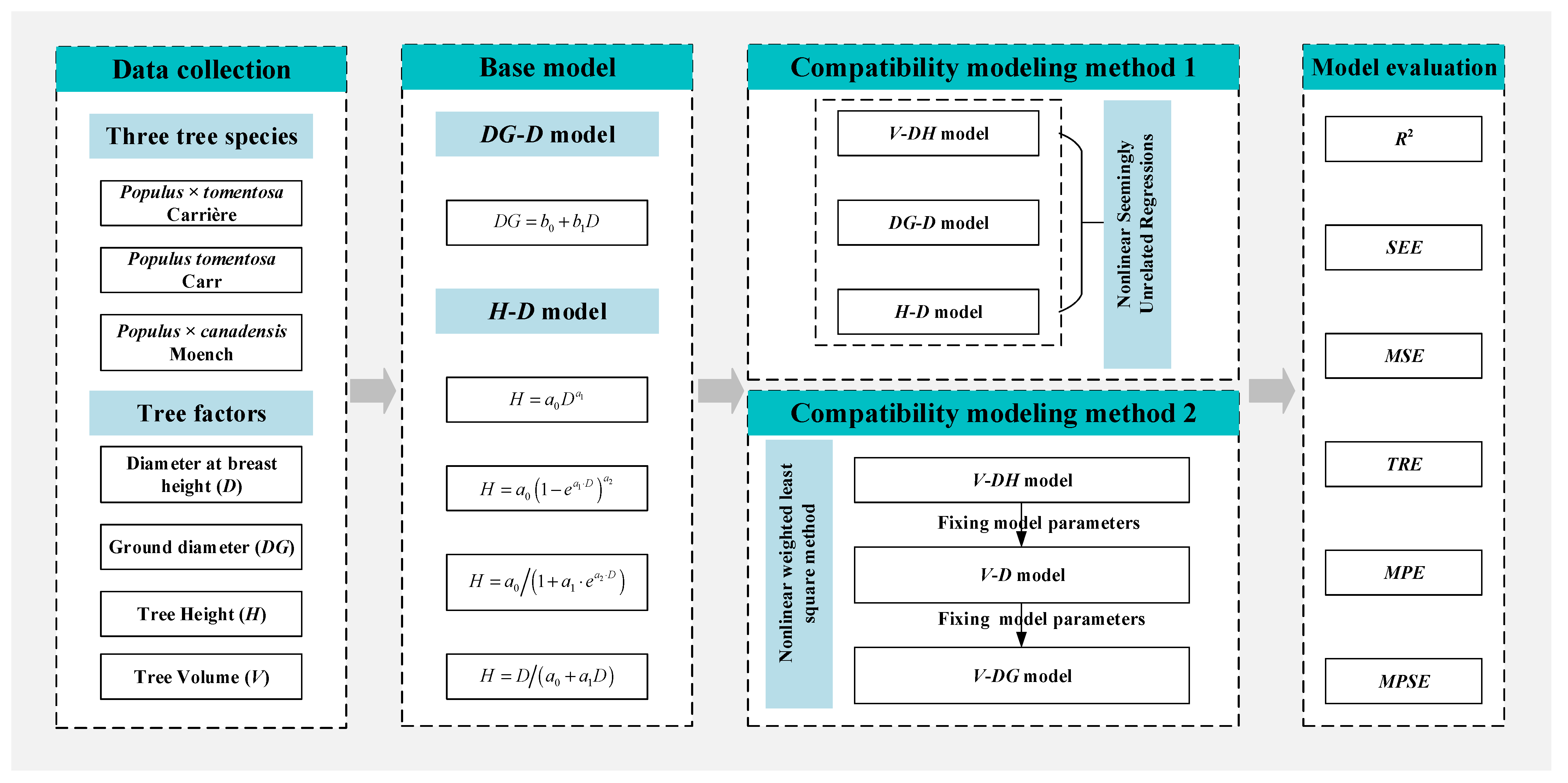
2.2.1. Model Form Selection

For the H-D model, the candidate model forms included the power function, Chapman–Richards function, and logistics function (Models 1–4). A linear function (Model 5) was employed for the DG-D model. The Schumacher and Hall volume equation (Model 6) was adopted for the V-DH model. The calculations for each model were as follows:

$$\mathrm{Model} 1: H=a_0{D}^{a_1},$$

$$\mathrm{Model} 2: H=a_0{\left(1-e^{a_1\cdot D}\right)}^{a_2},$$

$$\mathrm{Model} 3: H=a_0/\left(1+a_1\cdot e^{a_2\cdot D}\right),$$

$$\mathrm{Model} 4: H=D/\left(a_0+a_{1}D\right),$$

$$\mathrm{Model} 5: DG=b_0+b_{1}D, \mathrm{and}$$

$$\mathrm{Model} 6: V=c_0{D}^{c_1}{H}^{c_2}.$$

Akaike information criterion (AIC) statistics were used to assess the model complexity and its goodness of fit, with preference being given to models with smaller AIC values. Using the AIC minimization criterion, the optimal model form for the H-D model was selected.

2.2.2. Compatible Volume Model

In modeling V-DH, V-D, and V-DG volume models, it is typical to treat them independently, often disregarding their correlations. Fitting these models individually can lead to incompatibility of volume predictions. In this study, the H-D and DG-D models were employed as bridges, employing two compatible modeling methods to ensure the compatibility of the predicted results for all three of the volume models.

Compatibility method 1: The V-DH model was denoted as $\widehat{V}=f_1\left(D,H\right)$, the H-D model was denoted as $\widehat{H}=f_2\left(D\right)$, and the DG-D model was denoted as $\widehat{D}G=f_3\left(D\right)$. The error-in-variable simultaneous equations method was employed alongside a nonlinear seemingly unrelated regression to estimate the parameters, as follows:

$$\left\{\begin{array}{l}\widehat{V}=f_1\left(D,\widehat{H}\right)=c_0{D}^{c_1}{\widehat{H}}^{c_2}\\ \widehat{H}=f_2\left(D\right)\\ \widehat{D}G=f_3\left(D\right)\end{array}\right..$$

Using the estimation of value of $f_2\left(D\right)$, the V-D model was derived, i.e., $\widehat{V}=f_1\left(D,f_2\left(D\right)\right)$. The inverse function of $f_3\left(D\right)$ was obtained. The V-DG model was then derived, i.e., $\widehat{V}=f_1\left(f_3^{-1}\left(DG\right),f_2\left(f_3^{-1}\left(DG\right)\right)\right)$.

Compatibility method 2: The value of $V=a{D}^b{H}^c$ is fitted, and the parameters of the V-DH model were obtained. After the parameters of the V-DH model were determined, the H-D model, $H=g_1\left(D\right)$, was obtained by fitting the V-D model, i.e., $V=a{D}^b{\left(g_1\left(D\right)\right)}^c$. After fixing the parameters of the V-D model, the D-DG model, $D=g_2\left(DG\right)$, was obtained by fitting the V-DG model, i.e., $V=a{\left(g_2\left(DG\right)\right)}^b{\left(g_1\left(g_2\left(DG\right)\right)\right)}^c$. The inverse function of the D-DG model was the DG-D model.

2.2.3. Model Evaluation and Validation

This study employed all samples for modeling without distinguishing between the modeling and test samples. The six indicators for evaluating the regression models included the coefficient of determination (R²), standard error of estimates (SEE), total relative error (TRE), mean systematic error (MSE), mean estimated error (MPE), and mean percentage standard error (MPSE), as follows:

$$R^2=1-{\displaystyle \sum {(y_i-{\widehat{y}}_i)}^2/{\displaystyle \sum {(y_i-\overline{y})}^2}},$$

$$SEE=\sqrt{{\displaystyle \sum {(y_i-{\widehat{y}}_i)}^2}/(n-p)},$$

$$TRE={\displaystyle \sum (y_i-{\widehat{y}}_i)/{\displaystyle \sum {\widehat{y}}_i}}\times 100,$$

$$MSE={\displaystyle \sum (y_i-{\widehat{y}}_i)/{\widehat{y}}_i/n\times 100},$$

$$MPE=t_{\alpha }(SEE/\overline{y})/\sqrt{n}\times 100, \mathrm{and}$$

$$MPSE=\frac{1}{n}{\displaystyle \sum _{i=1}^n\left|(y_i-{\widehat{y}}_i)/{\widehat{y}}_i\right|\times 100},$$

where $y_i$ and ${\widehat{y}}_i$ denote the measured and estimated values of the i-th sample, respectively; $\overline{y}$ denotes the average of the measured value of all samples; n represents the number of samples; p represents the number of model parameters; and $t_{\alpha }$ represents the t-value of the n-p degrees of freedom and the 95% confidence level.

2.2.4. Correlation Analysis

The Pearson correlation coefficient was used to calculate the correlations between the variables. Nonmetric multidimensional scaling (NMDS) was used in this study, which simplifies multidimensional space to low-dimensional space. An analysis of similarities (ANOSIM) was used to test whether the differences in the trees between the groups were significantly greater than the differences in the trees within the groups based on Bray-Curtis distance.

Figure 1 illustrates the data collection and analysis process (Figure 1). All statistical calculations were conducted using R 4.3.1 [43], and parameter estimations were performed using the systemfit package [44].

3. Results

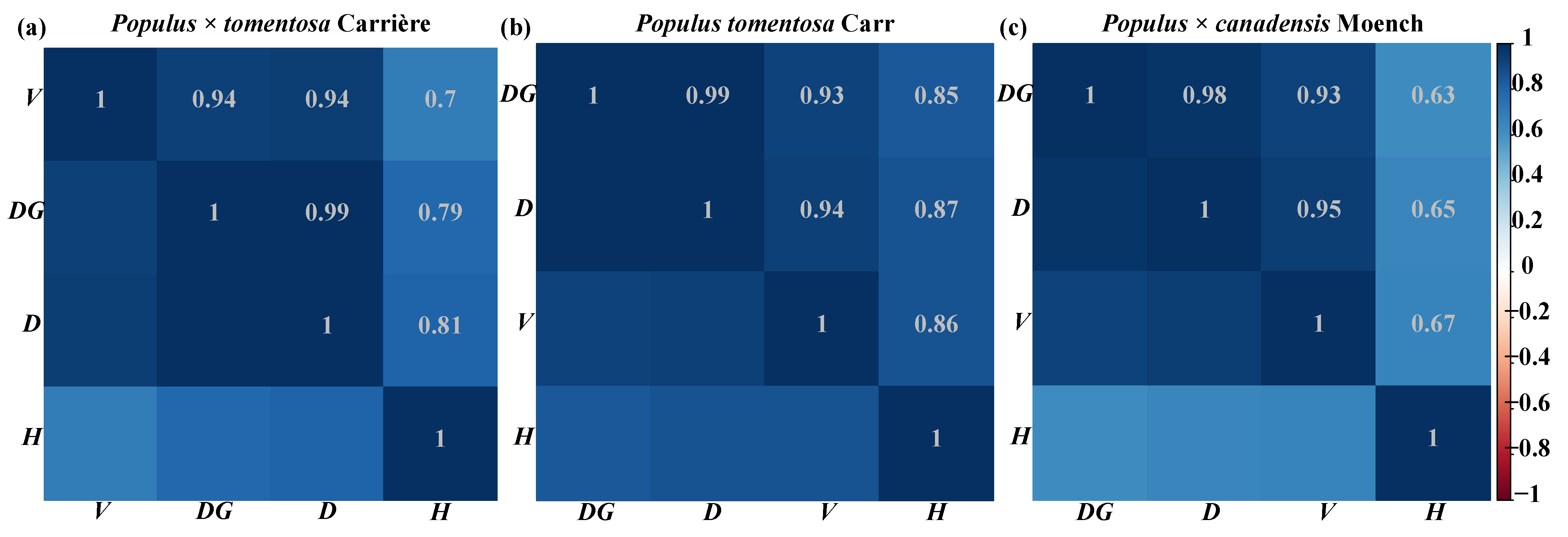
3.1. Correlation Analysis

The correlation analysis results are shown in Figure 2. DG, D, and H were positively correlated with V. The correlation between H and V was relatively low. The correlation coefficient for Populus × tomentosa Carrière ranged from 0.7 to 0.99. The correlation coefficient for Populus tomentosa Carr ranged from 0.85 to 0.99. The correlation coefficient for Populus × canadensis Moench ranged from 0.63 to 0.98 (Figure 3).

For the two-dimensional distribution figure of the NMDS, the stress value was 0.0366, demonstrating that the figure could accurately reflect the real differences for each tree (Figure 3). The confidence ellipse was obtained with a confidence level of 95%, which showed that the confidence ellipses of the different species overlapped, demonstrating similarity between the groups. The analysis of similarities based on the Bray–Curtis distance suggested that the difference between the species was significantly greater than the difference within the groups (R = 0.1827, p = 0.001).

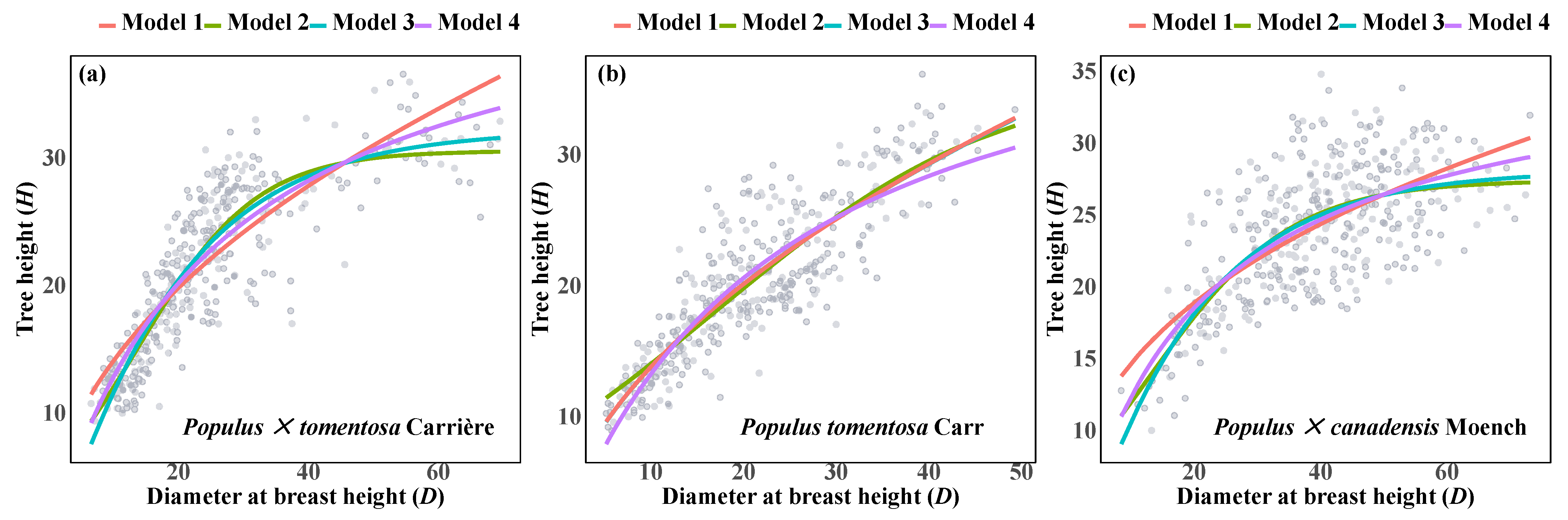
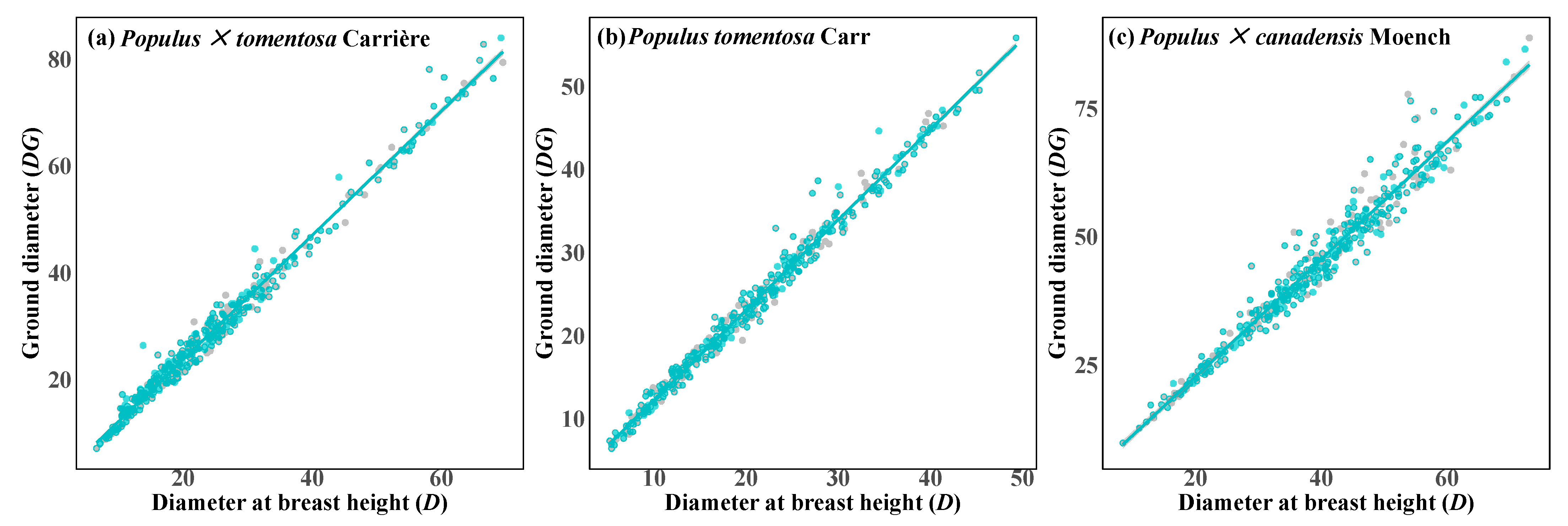
3.2. Independent Fitting Model Analysis

Model 3 exhibited the lowest AIC value (2018.225), indicating its superior performance in fitting the H-D model for Populus × tomentosa Carrière. Similarly, Model 1 demonstrated the lowest AIC value (1976.589), signifying its effectiveness in fitting the H-D model for Populus tomentosa Carr. For Populus × canadensis Moench, Model 2 achieved the lowest AIC value (2078.769), suggesting its optimal fit for the H-D model (

Table 2. Regression parameters (a₀, a₁, and a₂) and evaluation indicators (AIC and R²) for the four H-D candidate models (Models 1–4 in Section 2.2.1.) for the three tree species (Populus × tomentosa Carrière, Populus tomentosa Carr, and Populus × canadensis Moench).

Tree Species	Model	a0	a1	a2	AIC	R2
Populus × tomentosa Carrière	Model 1	4.724	0.4830	-	2109.006	0.7285
	Model 2	32.44	−0.06078	1.281	2020.619	0.7829
	Model 3	30.83	4.505	−0.1091	2018.225	0.7842
	Model 4	0.5527	0.02131	-	2042.76	0.7700
Populus tomentosa Carr	Model 1	4.080	0.5370	-	1976.589	0.7590
	Model 2	192.4	−7.984 × 10−4	0.5415	1978.77	0.7583
	Model 3	36.58	2.965	−0.06409	1990.518	0.7511
	Model 4	0.5223	0.02185	-	1998.562	0.7454
Populus × canadensis Moench	Model 1	6.470	0.362	-	2104.811	0.4720
	Model 2	28.32	−0.0601	1.214	2078.769	0.5065
	Model 3	27.63	3.067	−0.08843	2079.17	0.5060
	Model 4	0.5270	0.02696	-	2084.055	0.4987

Note: Akaike information criterion, AIC and coefficient of determination, R².

and Figure 4). Additionally, the R² values for Model 5 were 0.9848, 0.9868, and 0.9601 for Populus × tomentosa Carrière, Populus tomentosa Carr, and Populus × canadensis Moench, respectively. These values indicated that the linear model successfully explained over 96% of the variation in the DG-D relationship for all three tree species (

Table 3. Regression parameters (b₀ and b₁) and evaluation indicators (AIC and R²) for the DG-D model for the three tree species (Populus × tomentosa Carrière, Populus tomentosa Carr, and Populus × canadensis Moench).

Tree Species	Model	b0	b1	AIC	R2
Populus × tomentosa Carrière	Model 5	1.188	1.164	1659.307	0.9848
Populus tomentosa Carr	Model 5	1.825	1.087	1273.561	0.9868
Populus × canadensis Moench	Model 5	0.4705	1.146	2023.708	0.9601

Note: Akaike information criterion, AIC and coefficient of determination, R².

and Figure 5).

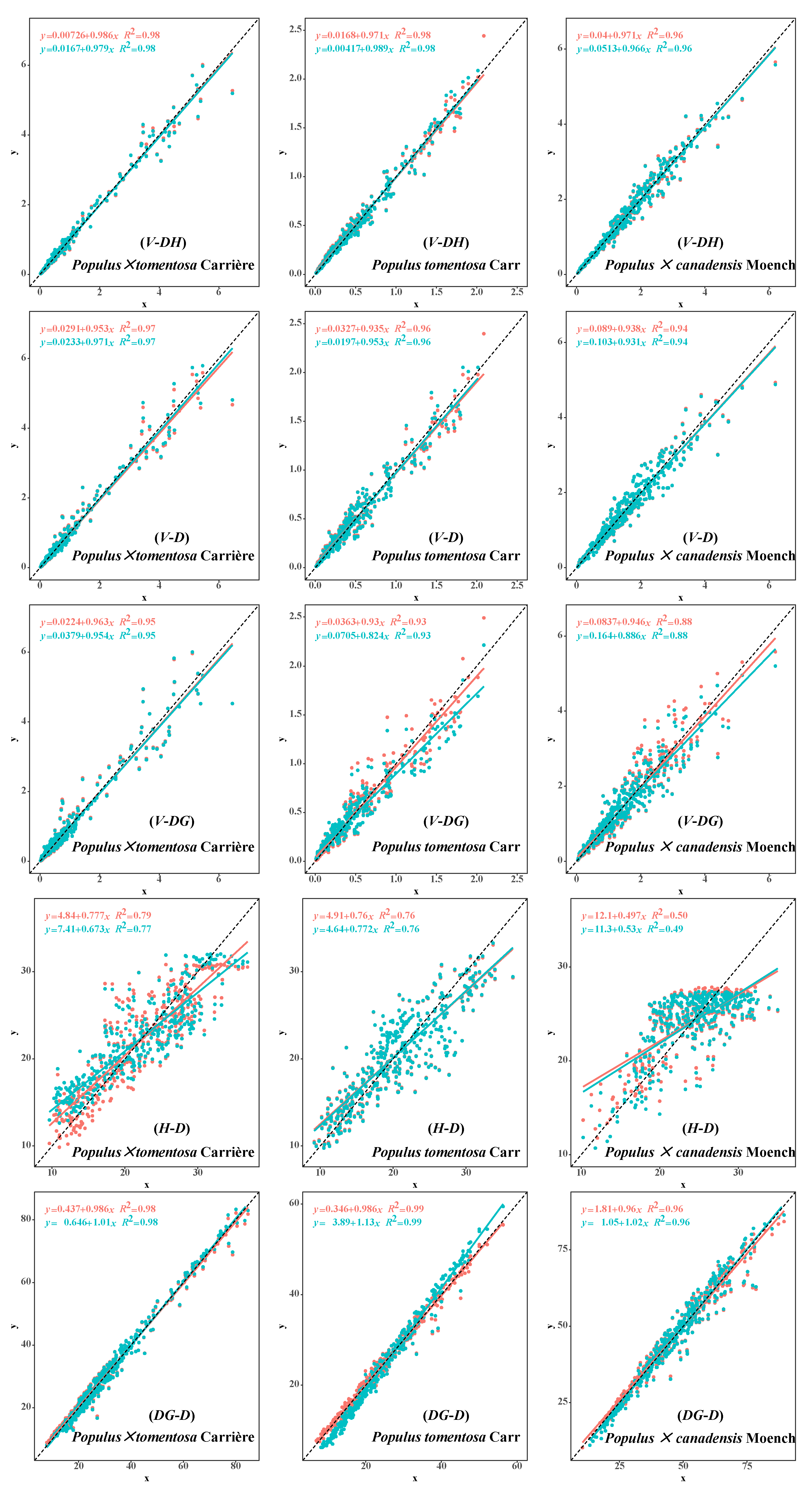
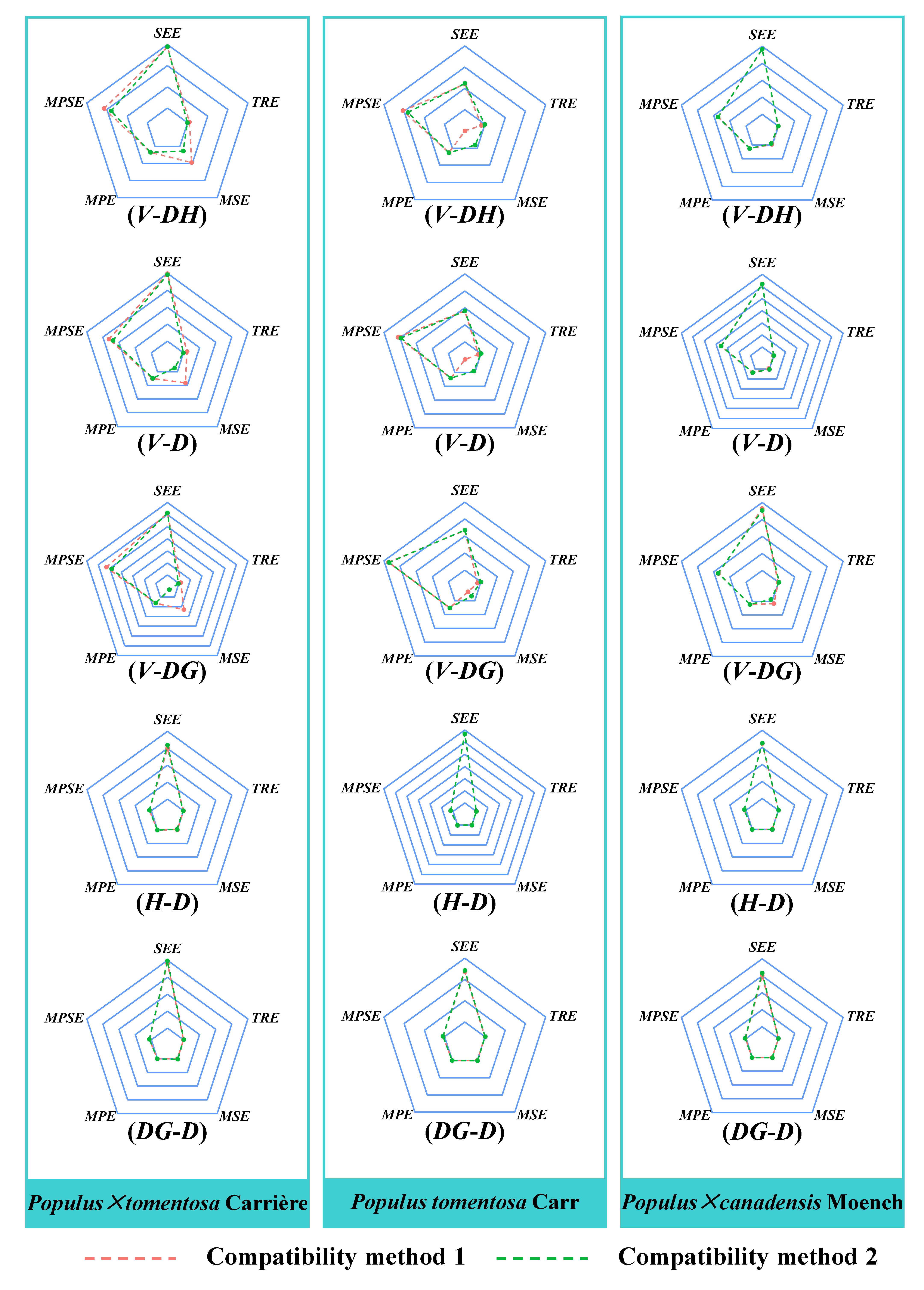
3.3. Analysis of the Two Compatibility Models

Two compatibility methods were utilized to fit the following three models: DG-D, H-D, and V-DH. The results revealed minimal disparity in the parameters between the V-DH and DG-D models, whereas significant differences existed in the parameters of the DG-D models (

Table 4. Parameter results (a₀, a₁, a₂, b₀, b₁, c₀, c₁, and c₂) for the three different models (V-DH model, H-D model, and DG-D model) for the three trees species (Populus × tomentosa Carrière, Populus tomentosa Carr, and Populus × canadensis Moench) under the two compatible modeling methods.

Tree Species	Compatible Method	H-D Model				DG-D Model			V-DH Model
		a0	a1	a2	Model	b0	b1	Model	c0	c1	c2	Model
Populus × tomentosa Carrière	(1)	30.92	4.313	−0.1063	(3)	1.166	1.165	(5)	0.00003218	2.029	1.009	(6)
	(2)	32.50	2.564	−0.07401	(3)	0.1035	1.197	(5)	0.00004648	2.051	0.8753	(6)
Populus tomentosa Carr	(1)	4.096	0.5358	-	(1)	1.843	1.086	(5)	0.00008537	1.750	0.9779	(6)
	(2)	3.971	0.5454	-	(1)	1.169	1.113	(5)	0.00005777	1.798	1.047	(6)
Populus × canadensis Moench	(1)	28.37	−0.05930	1.193	(2)	0.4694	1.146	(5)	0.00005659	1.996	0.8460	(6)
	(2)	27.54	−0.08152	2.047	(2)	−2.518	1.216	(5)	0.00006000	1.991	0.8341	(6)

Note: The models consisted of the following five types: V-DH, V-D, V-DG, H-D, and DG-D. Before the horizontal line was the dependent variable, and behind the horizontal line was the independent variable.

). Based on the V-DH model, the H-D and DG-D models served as bridges to infer the results of the V-D and V-DG models, thereby ensuring compatibility among the three volume models.

For Populus × tomentosa Carrière, the MPE values for the five models fell within the range of 0.62%–3.16%, suggesting an overall prediction accuracy exceeding 96.84%. For Populus tomentosa Carr, the MPE values for the five models varied from 0.47% to 2.57%, indicating an overall prediction accuracy of 97.43%. For Populus × canadensis Moench, the MPE values for the five models ranged from 0.65% to 2.40%, indicating an overall prediction accuracy exceeding 97.60% (

Table 5. Precision index (R², SEE, TRE, MSE, MPE, and MPSE) results for the five different models (V-DH model, V-D model, V-DG model, H-D model, and DG-D model) for the three tree species (Populus × tomentosa Carrière, Populus tomentosa Carr, and Populus × canadensis Moench) under the two compatible modeling methods.

Tree Species	Model	Compatibility Method	R2	SEE	TRE	MSE	MPE	MPSE
Populus × tomentosa Carrière	V-DH model	(1)	0.9840	0.1439	0.49%	4.75%	1.77%	10.75%
		(2)	0.9838	0.1448	−0.03%	1.37%	1.78%	8.97%
	H-D model	(1)	0.7851	2.9979	−0.03%	−0.13%	1.36%	11.00%
		(2)	0.7566	3.1909	−1.52%	−2.57%	1.45%	12.06%
	V-D model	(1)	0.9695	0.1996	1.08%	4.10%	2.46%	13.15%
		(2)	0.9704	0.1966	−0.02%	−1.37%	2.42%	11.89%
	DG-D model	(1)	0.9848	1.9160	−0.04%	0.11%	0.62%	5.48%
		(2)	0.9837	1.9824	0.85%	1.95%	0.64%	5.82%
	V-DG model	(1)	0.9501	0.2559	0.86%	6.57%	3.15%	21.54%
		(2)	0.9500	0.2563	−0.17%	−3.65%	3.16%	19.27%
Populus tomentosa Carr	V-DH model	(1)	0.9822	0.0599	−0.87%	−4.98%	1.31%	10.32%
		(2)	0.9812	0.0617	−0.06%	−0.89%	1.35%	9.04%
	H-D model	(1)	0.7596	2.8486	−0.01%	0.01%	1.36%	10.91%
		(2)	0.7595	2.8495	0.15%	0.29%	1.36%	10.94%
	V-D model	(1)	0.9590	0.0912	−0.77%	−4.84%	2.00%	15.63%
		(2)	0.9595	0.0908	0.00%	−0.53%	1.99%	14.76%
	DG-D model	(1)	0.9868	1.1830	−0.01%	−0.06%	0.47%	3.71%
		(2)	0.9861	1.2127	0.41%	1.00%	0.48%	3.94%
	V-DG model	(1)	0.9328	0.1172	−1.08%	−3.33%	2.57%	18.63%
		(2)	0.9326	0.1174	−0.06%	−1.69%	2.57%	18.46%
Populus × canadensis Moench	V-DH model	(1)	0.9650	0.1914	−0.01%	−0.23%	1.26%	8.64%
		(2)	0.9650	0.1914	−0.07%	−0.50%	1.26%	8.70%
	H-D model	(1)	0.5090	3.2326	−0.01%	0.00%	1.31%	10.98%
		(2)	0.4998	3.2627	0.45%	0.89%	1.33%	11.33%
	V-D model	(1)	0.9360	0.2597	−0.13%	−0.30%	1.71%	12.88%
		(2)	0.9359	0.2599	−0.01%	0.12%	1.71%	12.79%
	DG-D model	(1)	0.9602	3.0214	−0.01%	0.05%	0.65%	4.54%
		(2)	0.9563	3.1634	0.48%	1.67%	0.68%	5.58%
	V-DG model	(1)	0.8746	0.3645	−0.22%	1.66%	2.40%	16.98%
		(2)	0.8817	0.3539	0.37%	−1.31%	2.33%	17.24%

Note: The models consisted of the following five types: V-DH, V-D, V-DG, H-D, and DG-D. Before the horizontal line was the dependent variable, and behind the horizontal line was the independent variable. Note: coefficient of determination, R²; standard error of estimates, SEE; total relative error, TRE; mean systematic error, MSE; mean estimated error, MPE; and mean percentage standard error, MPSE.

).

Among the three volume models, the V-DH model demonstrated the highest performance level, with R² values ranging from 0.965 to 0.984 and MPE values ranging from 1.26% to 1.78%. The V-D model exhibited R² values between 0.9359 and 0.9704, with MPE values ranging from 1.71% to 2.46%. Finally, the V-DG model showed R² values ranging from 0.8746 to 0.9501 and MPE values ranging from 2.33% to 3.16%. For the tree H-D model, the R² values ranged from 0.4998 to 0.7851, with MPE values of between 1.31% and 1.45%. Conversely, the DG-D model showed R² values that ranged from 0.9563 to 0.9868 and MPE values that ranged from 0.47% to 0.68% (Table 5).

A comparative analysis revealed that compatibility method 2 outperformed compatibility method 1 among the three models. However, among the remaining 12 models, compatibility method 1 exhibited the best performance (Table 5, Figure 6 and Figure 7). Thus, the nonlinear seemingly uncorrelated regression (NSUR) was more effective.

4. Discussion

We observed differences in the preferences for the H-D model among the three species, with the logistic function proving more suitable for the H-D fitting of Populus × tomentosa Carrière, the Chapman–Richard function for Populus tomentosa Carr, and the power function for Populus × canadensis Moench. Various forms of the H-D model have existed, including the Chapman–Richards, logistic, Korf, and Gompertz functions [45,46], and there is no consensus on the optimal selection. Numerous studies have highlighted the superior performance of the Chapman–Richards model [47,48]. Given the fixed form of the H-D model, it would have been difficult to depict all possible H-D relationships across the different trees. In many permanent plots, although the D values for all the sampled trees could be commonly measured, only the H value of a subsample was recorded. Consequently, the H-D model could be frequently used to estimate the heights of other sampled trees. Hence, it may be essential to compare and select a suitable model form, develop an appropriate H-D model, and, subsequently, apply it to forest surveys.

Some studies have incorporated factors, such as site conditions and stand structures, into predictors within the H-D model, demonstrating better predictive accuracy than simple functions [49]. Nonlinear mixed-effects models offer greater efficiency and flexibility than least-squares regression by addressing the nested structure of data. For instance, Sharma et al. developed an H-D mixed-effect model utilizing stand dominance height, stand basal area, and stand density as site characteristics, achieving better fitting than the Chapman–Richards model [50]. Similarly, Bronisz et al. employed a mixed-effect model to investigate the impacts of stand density, productivity, and age on the H–D relationship [51]. Hence, there are plans to sample trees with varying site conditions and stand structures over a period of 3–5 years to establish an H-D mixed-effect model.

A robust volume model requires a substantial number of data samples to ensure its accuracy. When the sample size of a dataset is small, the accuracy of the model can be reduced. In this study, the dataset comprised 1200 samples, which was sufficient for constructing a volume model for the three tree species. Typically, volume model studies use sample sizes ranging from tens to hundreds [34,35]. For example, Zhang et al. developed a volume-biomass compatibility model based on data from 80 samples [29]. Subedi et al. derived a volume model from 48 sample trees in the western lowlands of Nepal [3]. Gimenez et al. employed non-destructive climbing techniques to measure 64 trees and established a volume model [19]. Similarly, Boczniewicz et al. developed a volume model by destructively sampling seventy-four trees across eight experimental sites in New Zealand [33].

Previous studies have typically fit univariate and bivariate volume models independently [52,53]. Each model can be estimated in isolation, ignoring the inherent correlations between tree factors. The drawback of this approach lies in the divergence of the predictions yielded by different volume models. For instance, previous studies have separately fitted taper and volume models, leading to significant discrepancies in trunk volumes [54].

An internationally recognized approach utilized by researchers involves integrating volume and taper models. A taper model predicts the diameter at a specified height, facilitating trunk volume determination through established formulas, such as Huber, Smalian, and Newton. When the integral of a taper model yields the same volume as that of a volume model, the compatibility between the two is confirmed [55]. For example, Boczniewicz established taper models for outer bark, inner bark, and heartwood to ensure compatibility with their respective volume models [33]. Similarly, Zhao et al. (2019) developed a fully compatible system for taper and volume models [56]. The advantage of employing a taper model is its ability to provide trunk volume and volume at any position through integration. However, this method requires tree harvesting and utilizes diameter data from various heights [33,34,35].

The compatible modeling method facilitates the synchronization of multiple response variables and finds widespread applications across various domains. However, its precise interpretation may vary across contexts. For instance, Zhang et al. (2016) developed a compatibility model system for aboveground biomass and volumes of poplar trees in Jiangsu Province, China [29]. Zeng and Tang (2012) constructed a compatibility model system for the aboveground biomass and volumes of Masson pine in China [30]. Zeng et al. (2011) devised a compatible biomass model for Pinus massoniana at different scales, ensuring that the sums of estimates from the small-scale model matched those of the large-scale model [57].

In this study, a compatible model system was established between the V-DH, V-D, and V-DG models to ensure consistency in the predicted values across the three volume models. Unlike other studies, the focus was on utilizing the tree H-D model and DG-D model as bridges, effectively linking the three volume models. Therefore, we emphasized the importance of prioritizing compatibility modeling to address potential incompatibility issues in future research, thereby enhancing the applicability and stability of the model.

The compatible volume model developed in this study demonstrated high prediction accuracy, with MPE values ranging from 1.26% to 3.16% for the V-DH, V-D, and V-DG models, indicating an overall prediction accuracy exceeding 96%. Numerous studies have employed MPE as a key metric to assess model accuracy [30,57]. The volume model established herein meets the precision standards necessary for compiling volume tables and can reliably predict the poplar volume in Beijing.

We observed that the V-DH model outperformed the V-D model, with the V-DG model ranking last. Numerous studies have shown that incorporating H as a predictor in volume models can significantly enhance model performance [22,29]. However, contrary to our findings, Zhang et al. discovered that adding H to a biomass model did not yield the anticipated improvements in model performance, particularly for branch and leaf biomass [29]. Moreover, diameters at various heights can exhibit varying capabilities in explaining volume variation, with overall volume variations better explained by D than DG [14,21,47]. Hence, for accurate volume estimation, researchers are advised to prioritize obtaining D, followed by H and DG.

We observed that the modeling procedures for the two compatible methods differed significantly but yielded similar parameter fitting results. Notably, the parameters of the DG-D model exhibited considerable variations. A precision comparison revealed that compatible method 1 outperformed compatible method 2. Method 1 utilized NSUR, which considered inter-model correlation and ensured compatibility, thereby facilitating effective parameter estimation. Numerous field studies have corroborated the methodological advantages of using NSUR [10,37,58]. Thus, it is recommended that NSUR be prioritized for practical applications.

The division of sample data into modeling and testing sets remains controversial. Some studies have suggested that evaluating model prediction solely based on modeling data accuracy results lacks persuasiveness, and they have advocated for testing the models used [59]. Conversely, Kozak et al. contended that testing samples for suitability might sacrifice modeling information without providing additional insights [60]. Zeng et al. further suggested combining test and modeling samples to prevent sample loss [61]. This study employed all samples for modeling without distinguishing between modeling and test samples. The model evaluation and validation were performed on full datasets. This can help to avoid the loss of sample amount during modeling.

Volume models provide accurate tree volume estimates, which are essential for the sustainable management of forest resources for middle- and long-term periods of time. The application of a volume model can predict tree volume in small-scale areas and forest volume stocks in large-scale areas, which is helpful for making reasonable cutting and tree species conservation plans. It is possible to apply the volume model developed for the three poplar species to other forest species, but it needs to be handled carefully. Firstly, the similarity between the new tree species and poplar in morphology would need to be evaluated. If the similarity is high, the applicability of the model will be strong. Secondly, field data collection and validation must be carried out to evaluate the accuracy of the model and to adjust the model’s parameters. This can save resources and time using existing models while contributing to the unified management of forest resources of multiple species, forming a comprehensive database to support ecological research.

5. Conclusions

Volume modeling research is crucial in forest tree conservation because it provides an accurate estimate of tree volume and helps in the development of scientific cutting and conservation plans. These models enable forest managers to determine the optimal times and methods for harvesting, ensuring that tree removal is sustainable. The volume models developed for the three populus species demonstrated both high accuracy and compatibility, offering valuable support for poplar wood resource assessments in Beijing. The introduction of the H-D model notably reduced the fieldwork labor costs. Our research revealed variations in the H-D model preferences across different tree species, with the logistic model proving optimal for the H-D fitting of Populus × tomentosa Carrière, with the Chapman–Richard model being optimal for Populus tomentosa Carr and the power function being optimal for Populus × canadensis Moench. Hence, practical applications should consider selecting H-D models based on tree species. We utilized two compatible modeling methods to construct five models, employing the H-D and DG-D models as bridges to ensure compatibility among the volume models. Among the three volume models, the V-DH model emerged as the superior choice, followed by the V-D and V-DG volume models, respectively. Therefore, the V-DH model can be considered preferable for practical applications. Additionally, our comparison of the compatibility methods revealed that the use of NSUR yielded a higher fitting accuracy.

This study employed error-in-variable simultaneous equations to address compatibility issues between volume models, with the parameters treated as fixed effects. Mixed-effects models incorporating both fixed and random effects have been popular. Future enhancements to volume model accuracy could involve integrating mixed-effect models with simultaneous equations and accounting for inter-plot variation.

References

1. Cervera, M.-T.; Storme, V.; Ivens, B.; Gusmao, J.; Liu, B.H.; Hostyn, V.; Van Slycken, J.; Van Montagu, M.; Boerjan, W. Dense Genetic Linkage Maps of Three Populus Species (Populus deltoides, P. nigra and P. trichocarpa) Based on AFLP and Microsatellite Markers. Genetics 2001, 158, 787–809. [Google Scholar] [CrossRef]
2. Liang, W.; Hu, H.; Liu, F.; Zhang, D. Research Advance of Biomass and Carbon Storage of Poplar in China. J. For. Res. 2006, 17, 75–79. [Google Scholar] [CrossRef]
3. Subedi, T.; Bhandari, S.K.; Pandey, N.; Timilsina, Y.P.; Mahatara, D. Form Factor and Volume Equations for Individual Trees of Shorea robusta in Western Low Land of Nepal Formfaktor-Und Volumengleichungen Für Den Salbaum (Shorea robusta) Im Westlichen Tiefland von Nepal. Austrian. J. For. Sci. 2021, 138, 143–166. [Google Scholar]
4. Oehmcke, S.; Li, L.; Trepekli, K.; Revenga, J.C.; Nord-Larsen, T.; Gieseke, F.; Igel, C. Deep Point Cloud Regression for Above-Ground Forest Biomass Estimation from Airborne LiDAR. Remote Sens. Environ. 2024, 302, 113968. [Google Scholar] [CrossRef]
5. Yao, Q.; Wang, J.; Zhang, J.; Xiong, N. Error Analysis of Measuring the Diameter, Tree Height, and Volume of Standing Tree Using Electronic Theodolite. Sustainability 2022, 14, 6950. [Google Scholar] [CrossRef]
6. Feng, Z.K.; Sui, H.D.; Deng, X.R.; Zang, S.Y. Survey and precision analysis of tree height by trigonometric leveling. J. Beijing For. Univ. 2007, 29, 31–35. (In Chinese) [Google Scholar]
7. Song, S.Y.; Wang, J.; Li, X.L.; Yin, H.L.; Feng, Z.K. Improvement of pressler method for stand volume measurement using electronic theodolite. Bull. Surv. Mapp. 2015, 7, 113–116. (In Chinese) [Google Scholar]
8. Basuki, T.M.; Van Laake, P.E.; Skidmore, A.K.; Hussin, Y.A. Allometric Equations for Estimating the Above-Ground Biomass in Tropical Lowland Dipterocarp Forests. For. Ecol. Manag. 2009, 257, 1684–1694. [Google Scholar] [CrossRef]
9. Chave, J.; Réjou-Méchain, M.; Búrquez, A.; Chidumayo, E.; Colgan, M.S.; Delitti, W.B.; Duque, A.; Eid, T.; Fearnside, P.M.; Goodman, R.C. Improved Allometric Models to Estimate the Aboveground Biomass of Tropical Trees. Glob. Chang. Biol. 2014, 20, 3177–3190. [Google Scholar] [CrossRef]
10. Liu, B.; Bu, W.; Zang, R. Improved Allometric Models to Estimate the Aboveground Biomass of Younger Secondary Tropical Forests. Glob. Ecol. Conserv. 2023, 41, e02359. [Google Scholar] [CrossRef]
11. Case, B.S.; Hall, R.J. Assessing Prediction Errors of Generalized Tree Biomass and Volume Equations for the Boreal Forest Region of West-Central Canada. Can. J. For. Res. 2008, 38, 878–889. [Google Scholar] [CrossRef]
12. Kenzo, T.; Ichie, T.; Hattori, D.; Itioka, T.; Handa, C.; Ohkubo, T.; Kendawang, J.J.; Nakamura, M.; Sakaguchi, M.; Takahashi, N. Development of Allometric Relationships for Accurate Estimation of Above-and below-Ground Biomass in Tropical Secondary Forests in Sarawak, Malaysia. J. Trop. Ecol. 2009, 25, 371–386. [Google Scholar] [CrossRef]
13. Diamantopoulou, M.J.; Özçelik, R.; Yavuz, H. Tree-Bark Volume Prediction via Machine Learning: A Case Study Based on Black Alder’s Tree-Bark Production. Comput. Electron. Agr. 2018, 151, 431–440. [Google Scholar] [CrossRef]
14. Diamantopoulou, M.J.; Milios, E. Modelling Total Volume of Dominant Pine Trees in Reforestations via Multivariate Analysis and Artificial Neural Network Models. Biosyst. Eng. 2010, 105, 306–315. [Google Scholar] [CrossRef]
15. Nieto, P.G.; Torres, J.M.; Fernández, M.A.; Galán, C.O. Support Vector Machines and Neural Networks Used to Evaluate Paper Manufactured Using Eucalyptus Globulus. Appl. Math. Model. 2012, 36, 6137–6145. [Google Scholar] [CrossRef]
16. Ogana, F.N.; Ercanli, I. Modelling Height-Diameter Relationships in Complex Tropical Rain Forest Ecosystems Using Deep Learning Algorithm. J. Forestry. Res. 2022, 33, 883–889. [Google Scholar] [CrossRef]
17. Sharma, M. Increasing Volumetric Prediction Accuracy—An Essential Prerequisite for End-Product Forecasting in Red Pine. Forests 2020, 11, 1050. [Google Scholar] [CrossRef]
18. Joosten, R.; Schumacher, J.; Wirth, C.; Schulte, A. Evaluating Tree Carbon Predictions for Beech (Fagus sylvatica L.) in Western Germany. For. Ecol. Manag. 2004, 189, 87–96. [Google Scholar] [CrossRef]
19. Gimenez, B.O.; Dos Santos, L.T.; Gebara, J.; Celes, C.H.; Durgante, F.M.; Lima, A.J.; Dos Santos, J.; Higuchi, N. Tree Climbing Techniques and Volume Equations for Eschweilera (Matá-Matá), a Hyperdominant Genus in the Amazon Forest. Forests 2017, 8, 154. [Google Scholar] [CrossRef]
20. Sharma, M. Total and Merchantable Volume Equations for 25 Commercial Tree Species Grown in Canada and the Northeastern United States. Forests 2021, 12, 1270. [Google Scholar] [CrossRef]
21. Hogg, B.W.; Lewis, T.; Huth, J.R.; Lee, D.J. Small-Tree Volume Equations for Subtropical Hardwood Plantation Species. Aust. Forestry. 2021, 84, 152–158. [Google Scholar] [CrossRef]
22. Tabacchi, G.; Di Cosmo, L.; Gasparini, P. Aboveground Tree Volume and Phytomass Prediction Equations for Forest Species in Italy. Eur. J. Forest. Res. 2011, 130, 911–934. [Google Scholar] [CrossRef]
23. Adame, P.; del Río, M.; Canellas, I. A Mixed Nonlinear Height–Diameter Model for Pyrenean Oak (Quercus pyrenaica Willd.). For. Ecol. Manag. 2008, 256, 88–98. [Google Scholar] [CrossRef]
24. Tian, X.; Sun, S.; Mola-Yudego, B.; Cao, T. Predicting Individual Tree Growth Using Stand-Level Simulation, Diameter Distribution, and Bayesian Calibration. Ann. Forest. Sci. 2020, 77, 57. [Google Scholar] [CrossRef]
25. Chukwu, O.; Osho, J.S. Basal Area-Stump Diameter Models for Tectona grandis Linn. f. Stands in Omo Forest Reserve, Nigeria. J. For. Environ. Sci. 2018, 34, 119–125. [Google Scholar]
26. Spurr, S.H. Forest Inventory. In Forest Inventory; Ronald Press Co.: New York, NY, USA, 1952. [Google Scholar]
27. Schumacher, F. Logarithmic Expression of Timber-Tree Volume. J. Agric. Res. 1933, 47, 719–734. [Google Scholar]
28. Fonweban, J.; Gardiner, B.; Auty, D. Variable-Top Merchantable Volume Equations for Scots Pine (Pinus sylvestris) and Sitka Spruce (Picea sitchensis (Bong.) Carr.) in Northern Britain. Forestry 2012, 85, 237–253. [Google Scholar] [CrossRef]
29. Zhang, C.; Peng, D.-L.; Huang, G.-S.; Zeng, W.-S. Developing Aboveground Biomass Equations Both Compatible with Tree Volume Equations and Additive Systems for Single-Trees in Poplar Plantations in Jiangsu Province, China. Forests 2016, 7, 32. [Google Scholar] [CrossRef]
30. Zeng, W.; Tang, S. Modeling Compatible Single-Tree Aboveground Biomass Equations for Masson Pine (Pinus massoniana) in Southern China. J. For. Res. 2012, 23, 593–598. [Google Scholar] [CrossRef]
31. Zianis, D.; Mencuccini, M. On Simplifying Allometric Analyses of Forest Biomass. For. Ecol. Manag. 2004, 187, 311–332. [Google Scholar] [CrossRef]
32. Zeng, W.; Zhang, L.; Chen, X.; Cheng, Z.; Ma, K.; Li, Z. Construction of Compatible and Additive Individual-Tree Biomass Models for Pinus tabulaeformis in China. Can. J. For. Res. 2017, 47, 467–475. [Google Scholar] [CrossRef]
33. Boczniewicz, D. Developing Fully Compatible Taper and Volume Equations for All Stem Components of Eucalyptus globoidea Blakely Trees in New Zealand. Ph.D. Thesis, University of Canterbury, Christchurch, New Zealand, 2023. [Google Scholar]
34. Li, D.; Jia, W.; Guo, H.; Sun, Y.; Wang, F. Compatible Taper and Volume Systems for Larix Olgensis and Larix Kaempferi in Northeast China. Eur. J. Forest. Res. 2023, 143, 65–79. [Google Scholar] [CrossRef]
35. Behling, M.; Koehler, H.S.; Behling, A. Compatibility between the Stem Volume and Taper Equations Volume for Black Wattle Trees. Floresta 2020, 50, e1518. [Google Scholar] [CrossRef]
36. Bi, H.; Turner, J.; Lambert, M.J. Additive Biomass Equations for Native Eucalypt Forest Trees of Temperate Australia. Trees 2004, 18, 467–479. [Google Scholar] [CrossRef]
37. Parresol, B.R. Additivity of Nonlinear Biomass Equations. Can. J. For. Res. 2001, 31, 865–878. [Google Scholar] [CrossRef]
38. Tang, S.; Li, Y.; Wang, Y. Simultaneous Equations, Error-in-Variable Models, and Model Integration in Systems Ecology. Ecol. Model. 2001, 142, 285–294. [Google Scholar] [CrossRef]
39. Greene, W.H. Econometric Analysis; Pearson Education India: Noida, India, 2003; ISBN 81-7758-684-X. [Google Scholar]
40. Xiong, N.; Qiao, Y.; Ren, H.; Zhang, L.; Chen, R.; Wang, J. Comparison of Parameter Estimation Methods Based on Two Additive Biomass Models with Small Samples. Forests 2023, 14, 1655. [Google Scholar] [CrossRef]
41. Fu, L.; Lei, Y.; Wang, G.; Bi, H.; Tang, S.; Song, X. Comparison of Seemingly Unrelated Regressions with Error-in-Variable Models for Developing a System of Nonlinear Additive Biomass Equations. Trees 2016, 30, 839–857. [Google Scholar] [CrossRef]
42. Wang, X.; Zhao, D.; Liu, G.; Yang, C.; Teskey, R.O. Additive Tree Biomass Equations for Betula platyphylla Suk. Plantations in Northeast China. Ann. Forest. Sci. 2018, 75, 60. [Google Scholar] [CrossRef]
43. R Core Team. R: A Language and Environment for Statistical Computing; R Foundation for Statistical Computing: Vienna, Austria, 2013. [Google Scholar]
44. Henningsen, A.; Hamann, J.D. Systemfit: A Package for Estimating Systems of Simultaneous Equations in R. J. Stat. Softw. 2008, 23, 1–40. [Google Scholar] [CrossRef]
45. Fang, Z.; Bailey, R.L. Height–Diameter Models for Tropical Forests on Hainan Island in Southern China. For. Ecol. Manag. 1998, 110, 315–327. [Google Scholar] [CrossRef]
46. Curtis, R.O. Height-Diameter and Height-Diameter-Age Equations for Second-Growth Douglas-Fir. Forest. Sci. 1967, 13, 365–375. [Google Scholar]
47. Popoola, V.D.; Uii, J.N. Nonlinear Height-Diameter Models for Tectona grandis (Linn. F.) in Mbavaa Forest Reserve, Benue State, Nigeria. J. Res. For. Wildl. Environ. 2023, 15, 20–27. [Google Scholar]
48. Shamaki, S.; Akindele, S.; Isah, A.; Mohammed, I. Height-Diameter Relationship Models for Teak (Tectona grandis) Plantation in Nimbia Forest Reserve, Nigeria. Asian J. Environ. Ecol. 2016, 1, 1–7. [Google Scholar] [CrossRef]
49. Zang, H.; Lei, X.; Zeng, W. Height–Diameter Equations for Larch Plantations in Northern and Northeastern China: A Comparison of the Mixed-Effects, Quantile Regression and Generalized Additive Models. For. Int. J. For. Res. 2016, 89, 434–445. [Google Scholar] [CrossRef]
50. Sharma, M.; Parton, J. Height–Diameter Equations for Boreal Tree Species in Ontario Using a Mixed-Effects Modeling Approach. For. Ecol. Manag. 2007, 249, 187–198. [Google Scholar] [CrossRef]
51. Bronisz, K.; Mehtätalo, L. Mixed-Effects Generalized Height–Diameter Model for Young Silver Birch Stands on Post-Agricultural Lands. For. Ecol. Manag. 2020, 460, 117901. [Google Scholar] [CrossRef]
52. Mugasha, W.A.; Eid, T.; Bollandsås, O.M.; Malimbwi, R.E.; Chamshama, S.A.O.; Zahabu, E.; Katani, J.Z. Allometric Models for Prediction of Above-and Belowground Biomass of Trees in the Miombo Woodlands of Tanzania. For. Ecol. Manag. 2013, 310, 87–101. [Google Scholar] [CrossRef]
53. Fradette, O.; Marty, C.; Tremblay, P.; Lord, D.; Boucher, J.-F. Allometric Equations for Estimating Biomass and Carbon Stocks in Afforested Open Woodlands with Black Spruce and Jack Pine, in the Eastern Canadian Boreal Forest. Forests 2021, 12, 59. [Google Scholar] [CrossRef]
54. Shahzad, M.K.; Hussain, A.; Jiang, L. A Model Form for Stem Taper and Volume Estimates of Asian White Birch (Betula platyphylla): A Major Commercial Tree Species of Northeast China. Can. J. For. Res. 2020, 50, 274–286. [Google Scholar] [CrossRef]
55. Demaerschalk, J.P. Converting Volume Equations to Compatible Taper Equations. Forest. Sci. 1972, 18, 241–245. [Google Scholar] [CrossRef]
56. Zhao, D.; Lynch, T.B.; Westfall, J.; Coulston, J.; Kane, M.; Adams, D.E. Compatibility, Development, and Estimation of Taper and Volume Equation Systems. Forest. Sci. 2019, 65, 1–13. [Google Scholar] [CrossRef]
57. Zeng, W.S.; Zhang, H.R.; Tang, S.Z. Using the Dummy Variable Model Approach to Construct Compatible Single-Tree Biomass Equations at Different Scales—A Case Study for Masson Pine (Pinus massoniana) in Southern China. Can. J. For. Res. 2011, 41, 1547–1554. [Google Scholar] [CrossRef]
58. Dong, L.; Zhang, L.; Li, F. A Compatible System of Biomass Equations for Three Conifer Species in Northeast, China. For. Ecol. Manag. 2014, 329, 306–317. [Google Scholar] [CrossRef]
59. Shao, J. Linear Model Selection by Cross-Validation. J. Am. Stat. Assoc. 1993, 88, 486–494. [Google Scholar] [CrossRef]
60. Kozak, A.; Kozak, R. Does Cross Validation Provide Additional Information in the Evaluation of Regression Models? Can. J. For. Res. 2003, 33, 976–987. [Google Scholar] [CrossRef]
61. Zeng, W.S.; Tang, S.Z. Goodness evaluation and precision analysis of tree biomass equations. Sci. Silvae Sin. 2011, 47, 106–113. (In Chinese) [Google Scholar]
Figure 1. Flowchart of the data collection and analysis process. Note: diameter at breast height (D), tree height (H), ground diameter (DG), tree volume (V), coefficient of determination (R2), standard error of estimates (SEE), total relative error (TRE), mean systematic error (MSE), mean estimated error (MPE), and mean percentage standard error (MPSE).
Forests 15 01059 g001
Figure 2. Correlation heat map of the four variables (diameter at breast height [D], tree height [H], ground diameter [DG], and tree volume [V]). Blue indicates positive correlations. The deeper the blue, the larger the positive correlation value.
Forests 15 01059 g002
Figure 3. Non-metric multidimensional scaling (NMDS) analysis based on the Bray–Curtis dissimilarity. Each point represents a sample tree. The different colors represent the different species. The ellipses represent the 95% confidence intervals. Note: NMDS1, the first axis of the NMDS, and NMDS2, the second axis of the NMDS.
Forests 15 01059 g003
Figure 4. Regression results for the four H-D candidate models (Models 1–4) of the three tree species (Populus × tomentosa Carrière (a), Populus tomentosa Carr (b), and Populus × canadensis Moench (c)).
Forests 15 01059 g004
Figure 5. Regression results for the DG-D model for the three tree species (Populus × tomentosa Carrière, Populus tomentosa Carr, and Populus × canadensis Moench).
Forests 15 01059 g005
Figure 6. Fitting results for the measured volume values and predicted volume values for the five models (V-DH model, V-D model, V-DG model, H-D model, and DG-D model) for the three tree species (Populus × tomentosa Carrière, Populus tomentosa Carr, and Populus × canadensis Moench) under the two compatible modeling methods. The x axis is the measured value and the y axis is the predicted value of the model.
Forests 15 01059 g006
Figure 7. Radar map of the accuracy results for the five models (V-DH model, V-D model, V-DG model, H-D model, and DG-D model) for the three tree species (Populus × tomentosa Carrière, Populus tomentosa Carr, and Populus × canadensis Moench) under the two compatible modeling methods. Note: standard error of estimates, SEE; total relative error, TRE; mean systematic error, MSE; mean estimated error, MPE; and mean percentage standard error, MPSE.
Forests 15 01059 g007