Article

The Effects of Different Vegetation Restoration Models on Soil Quality in Karst Areas of Southwest China

1
Guangxi Key Laboratory of Superior Trees Resource Cultivation, Guangxi Zhuang Autonomous Region Forestry Research Institute, Nanning 530002, China
2
Huanjiang Observation and Research Station for Karst Ecosystems, Chinese Academy of Sciences, Hechi 547100, China
*
Author to whom correspondence should be addressed.
These authors contributed equally to this work.
Forests 2024, 15(6), 1061; https://doi.org/10.3390/f15061061
Submission received: 16 May 2024 / Revised: 10 June 2024 / Accepted: 12 June 2024 / Published: 19 June 2024

Abstract

:
Rocky desertification is a devastating process in Karst areas of Southwest China and induces serious fragmentation in ecosystems. Therefore, vegetation restoration and the scientific evaluation of soil quality are key restorative strategies in these areas. In this study, a natural closed forest and a disturbed forest with three restoration models, including an evergreen broad-leaved forest, mixed forest, and deciduous forest, were investigated in Huanjiang County. More than nineteen soil properties (including physical, chemical, and biotic properties) were analyzed across treatments, and principal component analyses (PCA) were combined with a minimum data set (MDS) applied to evaluate the soil quality. Our study sought to identify a vegetation restoration model to improve the soil quality in this area. We demonstrated that soil physical and chemical properties, microbial biomass, and enzyme activities significantly differed across all of the models. Soil water content, capillary porosity, total porosity, organic carbon, total phosphorus, available phosphorus, and urease activity were high in the mixed forest, leading to better physical soil properties. Also, relatively high soil total nitrogen, total potassium, available nitrogen, available potassium, microbial biomass C and N, catalase, sucrose, and alkaline phosphatase levels were observed in the deciduous broad-leaved forest, resulting in improved soil chemical properties. Based on the minimum data set (MDS) method, six indicators, including non-capillary porosity, organic carbon, total phosphorus, pH, microbial biomass nitrogen, and urease activity, were selected to evaluate the soil quality across the models. Our data showed that, among the five models, the deciduous broad-leaved forest had the highest soil quality index (0.618), followed by the mixed forest (0.593). Stepwise regression analysis showed that soil organic carbon explained 79.9% of the variations in the soil quality indices, suggesting it was a major factor affecting the soil quality. Thus, vegetation restoration models mainly comprised of native tree species effectively improved the soil quality in Karst rocky desertification areas, with deciduous broad-leaved forests displaying the best effects, followed by mixed forests.

1. Introduction

Forest soils are central elements of forest ecosystems, providing essential living conditions for forest vegetation, comprising water, fertilizer, gas, and heat. Soils underpin forest vegetation and are a vital hub for the transformation of nutrient elements in ecosystems, thereby promoting forest health [1]. Soil qualities (physical, chemical, and biological) are exemplified by their ability to maintain biological productivity, protect environmental quality, and support animal and plant health in diverse ecosystems [2,3]. Investigating forest soil quality provides indispensable scientific information for the health management of forests and the sustainable use of forest soil resources. The Karst area in Southwest China has a subtropical monsoon climate, with a high precipitation and air temperature rich in rain and heat resources, but is unevenly distributed. The area is also characterized by high rock exposure rates, thin and discontinuous soil layers, and sticky and heavy soil textures of low fertility. Most of the plants are calciphilic and drought-tolerant, and the climax community is defined by non-zonal evergreen or deciduous broad-leaved forests. With increased human disturbance and unreasonable land-use, most soils have degraded, leading to devastating rocky desertification, compromised stability, and a failure of local ecosystems to restore the natural order [4,5].
Vegetation restoration not only conserves the amount of water and soil and reduces soil erosion, but also improves the soil quality via soil–plant interaction, which are key steps vital for rocky desertification management and ecological reconstruction [6]. Characterized by strong adaptability, resistance, and economical value, native tree species display positive roles in stabilizing local ecosystems and are invaluable contributors to constructing local forest communities. Therefore, the restoration of local ecosystems using native- or local-tree-species-dependent vegetation restoration models is expected to be highly beneficial [7,8].
In terms of assessing land productivity, soil quality evaluation is highly relevant in assessing rocky desertification management programs. Recently, considerable efforts have been made to understand the effects of different vegetation restoration strategies on the soil quality in Karst rocky desertification areas. However, most studies have focused on the effects of different vegetation restoration models on single or a few soil parameters, including soil organic carbon (SOC) [9,10,11], the soil nitrogen cycle [12,13,14], soil physical properties [15,16], soil nutrients [4,17], and soil microbial communities [18,19,20]. The systemic evaluation of vegetation restoration effects on the soil quality in Karst areas has been limited, mostly investigating crops, economic forest tree species [21,22], and fast-growing introduced species [23], which served as vegetation restoration models. However, investigations on the effects of vegetation restoration models with native tree species on the soil quality in Karst areas are lacking; therefore, we investigated if our models could effectively improve the soil quality in these areas to facilitate ecosystem restoration.
In view of these reasons, we used common native tree species to construct the following three restoration models: (1) evergreen broad-leaved (EF), (2) mixed forest (MF), (3) and deciduous broad-leaved forest (DBF). We also conducted comparative studies using natural closed forest (NF) and disturbed forest (DF) systems. We analyzed differences in the physical and chemical soil properties, microbial biomass carbon and nitrogen levels, and soil enzyme activities across the restoration models. We systematically evaluated the soil quality of the vegetation restoration using minimum data set (MDS) methods. Our study objectives were (1) to identify the restoration model(s) which improved the soil quality in Karst rocky desertification areas as compared to conventional vegetation restoration strategies, and (2) to identify the key factors affecting the soil quality in these areas.

2. Materials and Methods
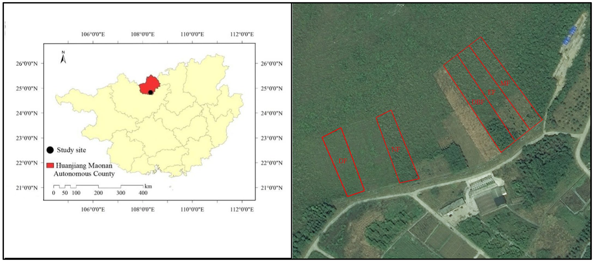
2.1. Study Areas

The study was performed in the Mulian comprehensive experimental demonstration site at the Huanjiang Observation and Research Station for Karst Ecosystem, Chinese Academy of Sciences, Huanjiang Maonan Autonomous County, Guangxi Zhuang Autonomous Region (108°18′05″–108°19′39″ E, 24°43′33″–24°44′25″ N), North Guangxi, China (Figure 1). The area has a subtropical monsoon climate with an average annual temperature of 19.9 °C, a mean annual precipitation of 1389.1 mm, sunshine hours of 1600–1800 h, and a mean relative humidity of 82%. The area is a typical Karst peak-cluster-depression region with altitudes between 272.0 and 647.2 m, with dark or brown calcareous soil. Exposed bedrock areas in the depression account for 15% of the land area, with a soil depth of 20–160 cm, whereas the exposed bedrock areas in sloping fields account for >30% of the land area, with a thin soil layer of 10–50 cm. Due to problems with transportation and farming management, all residents of the study area moved out in 1985, and the cultivated land was abandoned. Under the influence of burning, felling, and grazing, barren grasslands and sparse shrubs have become the main vegetation types in the study area, but there are dense shrub or secondary forests with a patchy and banded distribution on the hillsides, on both sides of the low-lying streams, and in the foothills around the slopes [24].
At the end of 2006, five vegetation restoration models, the EF, MF, DBF, NF, and DF, were established in five study plots (Figure 1), all of which were 20 m wide [24]. Before the study commencement, all of the study areas were previously wasteland, and the vegetation types were barren grassland and sparse shrub. According to the preliminary investigation, Zenia insignis Chun. is the pioneer tree of afforestation in the Karst area of China, and Choerospondias axillaris (Roxb.) Burtt et Hill and Cyclobalanopsis glauca (Thunb.) Oerst. are the dominant tree species in the top community. Therefore, we chose these three tree species for the vegetation restoration experiment. For the MF model, we selected three tree species, C. axillaris, Z. insignis, and C. glauca. The ratio of C. axillaris to Z. insignis was 5, and the ratio of C. glauca to Z. insignis was 4. For the EF model, we planted only C. glauca; for the DBF model, we planted Z. insignis and C. axillaris, and the ratio of Z. insignis to C. axillaris was 3. After afforestation, the stand density was controlled at 1100~1550 plants per hectare. The MF, EF, and DBF test sites were closely linked, with the NF at 100 m apart and the DF at 40 m apart.

2.2. Soil Sampling and Analysis

In August 2019, based on field investigations, five representative blocks with an area of 10 m × 10 m in stands of each of the five vegetation restoration types (total = 25 blocks) were established to collect basic information and soil samples. Soil profiles were obtained at the four corners and the center of each block (five soil profiles), with soils sampled at depths of 0–20 and 20–40 cm. Soils from the same block and same layer were mixed for laboratory analysis, with a total of 50 samples collected from 25 blocks. Soil samples were divided into two. One sample was stored at 4 °C after sieving through 2 mm steel screens, and was used to determine the soil enzyme activities and microbial biomass. The other sample was air-dried and passed through 2 mm sieves to measure the soil chemical properties. In terms of the soil profiles, undisturbed soil at depths of 0–20 cm and 20–40 cm was collected using a cutting ring (diameter = 50.46 mm, height = 50 mm, volume = 100 cm3) to evaluate the soil physical properties. Basic plot information is shown in Table 1.
As described, the soil bulk density (BD), non-capillary porosity (NCP), capillary porosity (CP), and total porosity (TPO) were determined using the cutting ring method. Soil natural moisture content (MC) was measured using the drying method [25].
Soil pH was measured by a glass electrode method on a soil/water suspension (1:2.5 ratio) [26]. Soil organic carbon (SOC) was measured by the potassium dichromate oxidation heating method (0.4 mol/L potassium dichromate solution as an extraction agent) [26]. Total nitrogen (TN) was determined by the Kjeldahl method with an automatic Kjeldahl apparatus (SKD-1000, PEiOU, Shanghai, China) [26]. Soil total phosphorus (TP) and total potassium (TK) were measured by spectrophotometry after wet digestion with HF-HClO4 [26]. Available nitrogen (AN) was measured by the NaOH hydrolysis diffusion method (1.8 mol/L NaOH solution as hydrolytic agent) [27]. Available phosphorus (AP) was assayed by a spectrophotometer (UV2600 UV–VIS, Tianmei, Shanghai, China) using a colorimetric method (0.5 M NaHCO3 solution as an extraction agent) [27]. Available potassium (AK) was assayed by the flame photometry (FP640, Huayan, Shanghai, China) method with 1.0 mol/L CH3COONH4 solution as an extraction agent [27].
The soil microbial biomass carbon (MBC) and microbial biomass nitrogen (MBN) were measured by chloroform fumigation. Soil, weighed in four portions (10.00 g × 4), was placed in a vacuum dryer containing chloroform and incubated at 25 °C for 24 h. Soil samples before and after fumigation were mixed with aqueous K2SO4 (0.5 mol/L, 40 mL), shaken at 300 rpm for 30 min, and filtered. The filtrate was measured on a multi-N/C 3100 (Analytik Jena AG, Jena, Germany) instrument [28,29].
Soil alkaline phosphatase (ALP) activity was determined using a Micro Soil Alkaline Phosphatase (S-ALP) Assay Kit (50T/48S, Beijing Solarbio Science & Technology Co., Ltd., Beijing, China) [30]. Soil catalase (CAT) activity was determined using a Micro Soil Catalase (S-CAT) Assay Kit (50T/24S, Beijing Solarbio Science & Technology Co., Ltd., Beijing, China) [30]. Soil urease (URE) activity was determined using a Micro Soil Urease (S-UE) Assay Kit (100T/48S, Beijing Solarbio Science & Technology Co., Ltd., Beijing, China) [30]. Soil sucrase (SAC) activity was determined using a Micro Soil Sucrase (S-SC) Assay Kit (50T/24S, Beijing Solarbio Science & Technology Co., Ltd., Beijing, China) [30].

2.3. Evaluation of Soil Quality Index (SQI)

In recent years, SQI evaluations have been widely used to quantitatively evaluate soil quality [21,23,31]. Principal component analyses (PCAs) have also been used to reduce the dimensions of the studied indicators, with principal components with eigenvalues ≥1 and total variations >5% being selected. Within each principal component, only factors whose absolute load value was <10% of the maximum factor loading was selected as an important indicator. When more than one important indicator existed in the principal component, Pearson correlation analysis was used to determine whether other indicators should be deleted. If relatively high correlations were observed between indicators (a correlation coefficient >0.6), only indicators with the highest absolute load value were retained in the principal component, and the minimum data set (MDS) was then established.
After determining the MDS, soil indicators were standardized using nonlinear scoring functions for normalization. In addition, the weight coefficient of each indicator in the MDS was determined using PCA (the proportion of the common factor variance of each indicator calculated by the PCA method to the sum of the common factor variance of all indicators). The formula for the nonlinear scoring function is [21,23] as follows:
S i = a / 1 + X i / X 0 i b
where i refers to one indicator in the MDS, Si is the score of the soil indicator i, a indicates the highest score (a = 1), Xi is every measurement of the indicator i, X0i represents the average soil indicator i, and b is the slope of the equation.
Finally, the SQI was calculated using the following equation according to the score and weight coefficient of each indicator in the MDS [21,23]:
S Q I = i = 1 n S i × W i
where Wi is the weight coefficient of the indicator i in the MDS as determined by PCA, Si is the score of soil indicators i, and n indicates the number of indicators in the MDS. SQI values were between 0 and 1; the higher the value, the better the soil quality.

2.4. Statistical Analyses

Routine statistics and graphs for soil indicators in different models were performed in Excel 2016. IBM SPSS Statistics 19.0 was used to perform the ANOVA and multiple comparisons (Duncan’s new multiple-range test, DMRT) of the soil indicators in different models. Soil indicators were screened and weighted using PCA and Pearson correlation analysis. A linear regression model was established with each soil indicator in the MDS as independent variables and the SQI as the dependent variable using stepwise regression analysis. All statistical analyses were performed at the 0.05 significance level (p < 0.05).

3. Results

3.1. Soil Physical and Chemical Properties in Models

Soil physical properties across the models are shown in Table 2. The F-value at p < 0.01 was different between the test members. The soil MC was reduced with an increasing soil depth in all of the models. The highest MC was observed in the MF model at 36.18%, 28.17%, and 32.18% levels at 0–20 cm, 20–40 cm, and 0–40 cm depths, respectively. These were significantly higher than the DBF, NF, and DF models. The soil BD was elevated with an increasing soil depth in all of the models. The DF model exhibited the highest BD at depths of 0–20 cm (1.15 g/cm3) and 0–40 cm (1.18 g/cm3), and the NF model had the highest BD at 1.24 g/cm3 at a depth of 20–40 cm. The lowest BD at all three depths was observed in the MF model at 0.81 g/cm3, 0.91 g/cm3, and 0.86 g/cm3 at 0–20 cm, 20–40 cm, and 0–40 cm, respectively.
The soil NCP levels in the EF and MF models were decreased with an increasing soil depth, while this level was increased in the DBF, NF, and DF models. The largest NCP was observed in the NF model at 8.90%, 7.89%, and 8.40% at 0–20 cm, 20–40 cm, and 0–40 cm depths, respectively. These were significantly higher than the other four models. The CP and TPO levels of all five models were reduced as the soil depths increased; the MF values were significantly higher than the other four models at all soil depths. Additionally, the DF model exhibited the lowest CP and TPO levels at all soil depths.
Soil chemical properties across the different models are shown in Table 3. The F-value at p < 0.01 was different between the test members. The SOC, TN, TK, TP, AN, AP, and AK were all reduced with an increasing soil depth in all of the models. At a depth of 0–20 cm, among the five vegetation models, the DBF model exhibited the highest SOC at 90.39 g/kg, but there were no significant differences in the SOC between the DBF and EF, and MF and NF modes. At depths of 20–40 cm and 0–40 cm, the highest SOC was observed in the MF model at 74.16 g/kg and 82.05 g/kg, respectively. The lowest SOC at 73.68 g/kg, 39.09 g/kg, and 56.39 g/kg at depths of 0–20 cm, 20–40 cm, and 0–40 cm, respectively, was observed in the DF model, which was substantially lower than the other models.
The DBF and DF models had the highest and lowest TN, TK, AN, and AK values in all soil layers. The TP and AP values in the MF model were the highest at all depths. The lowest TP value was observed in the NF model at 0–20 cm, and the DF model at 20–40 cm and 0–40 cm. In addition, the lowest AP value at all depths was observed in the DF model. The soil pH was elevated with an increasing soil depth in all models. The NF model had the highest pH at all three depths, the EF model had the lowest pH at a depth of 0–20 cm, and the MF model had the lowest pH at depths of 20–40 cm and 0–40 cm. No significant differences were observed in the pH values between the EF and MF models at all soil depths, and neither were the pH values among the DBF, NF, and DF vegetation models.
The pH of the EF model soil was the lowest in the 0–20 cm soil layer and, in the MF model soil, it was the lowest in the 20–40 cm and 0–40 cm soil layers.

3.2. Soil Microbial Biomass in Models

The soil MBC and MBN in the models are shown in Figure 2. The MBC and MBN were significantly different among the models at all soil layers (p < 0.01). The MBC and MBN were decreased with an increasing soil depth across the models, expect for the MBN in the MF model, which showed the opposite pattern. At the 0–20 cm and 20–40 cm levels, both the MBC and MBN shared the same order of DBF > MF > NF > EF > DF, whereas, at the layer of 0–40 cm, the order of the MBC and MBN was DBF > MF > NF > EF > DF and DBF > NF > MF > EF > DF, respectively.

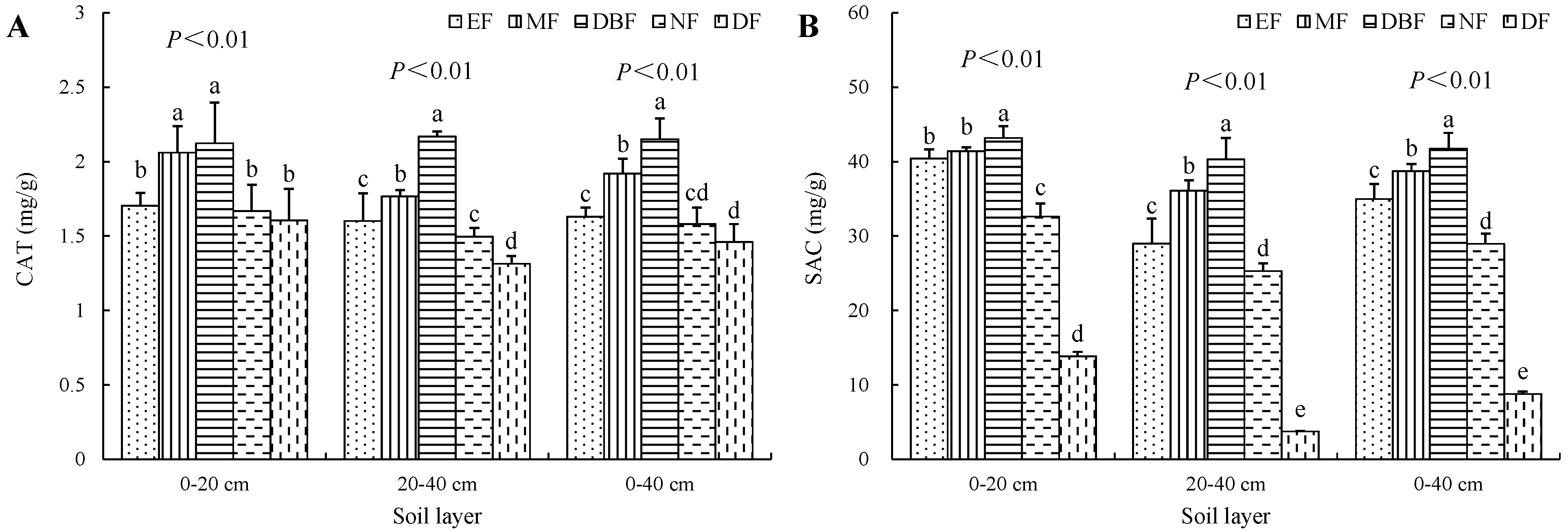
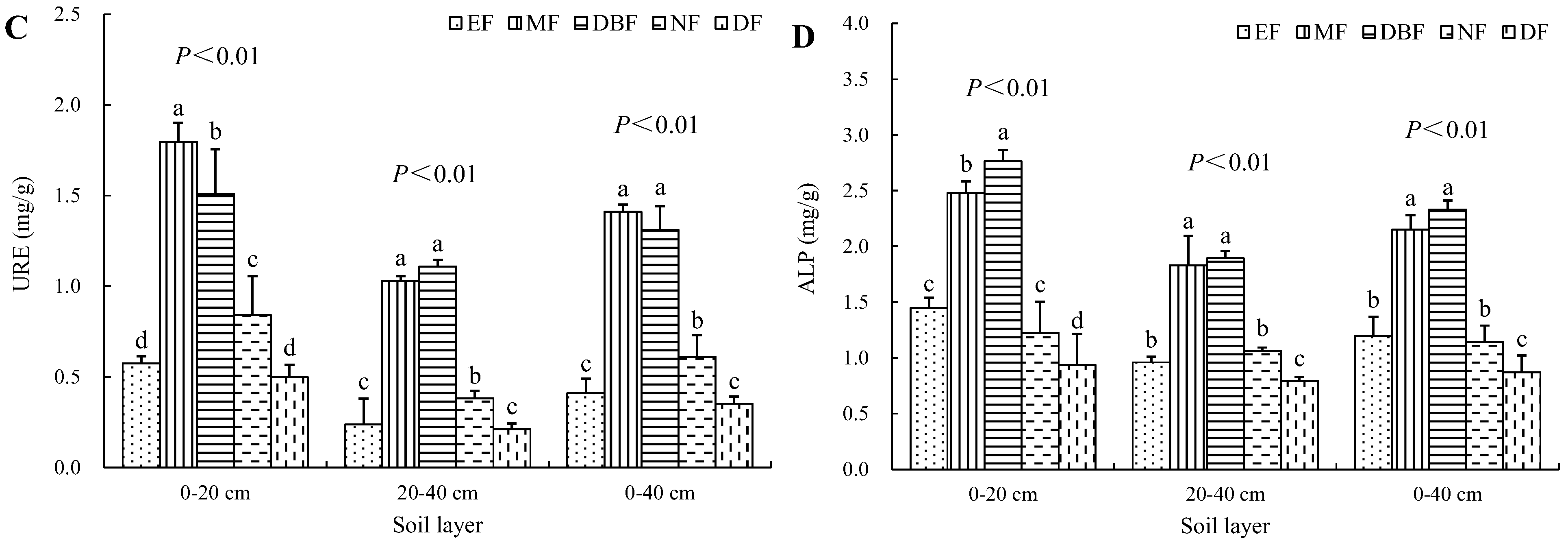
3.3. Soil Enzyme Activities in Restoration Models
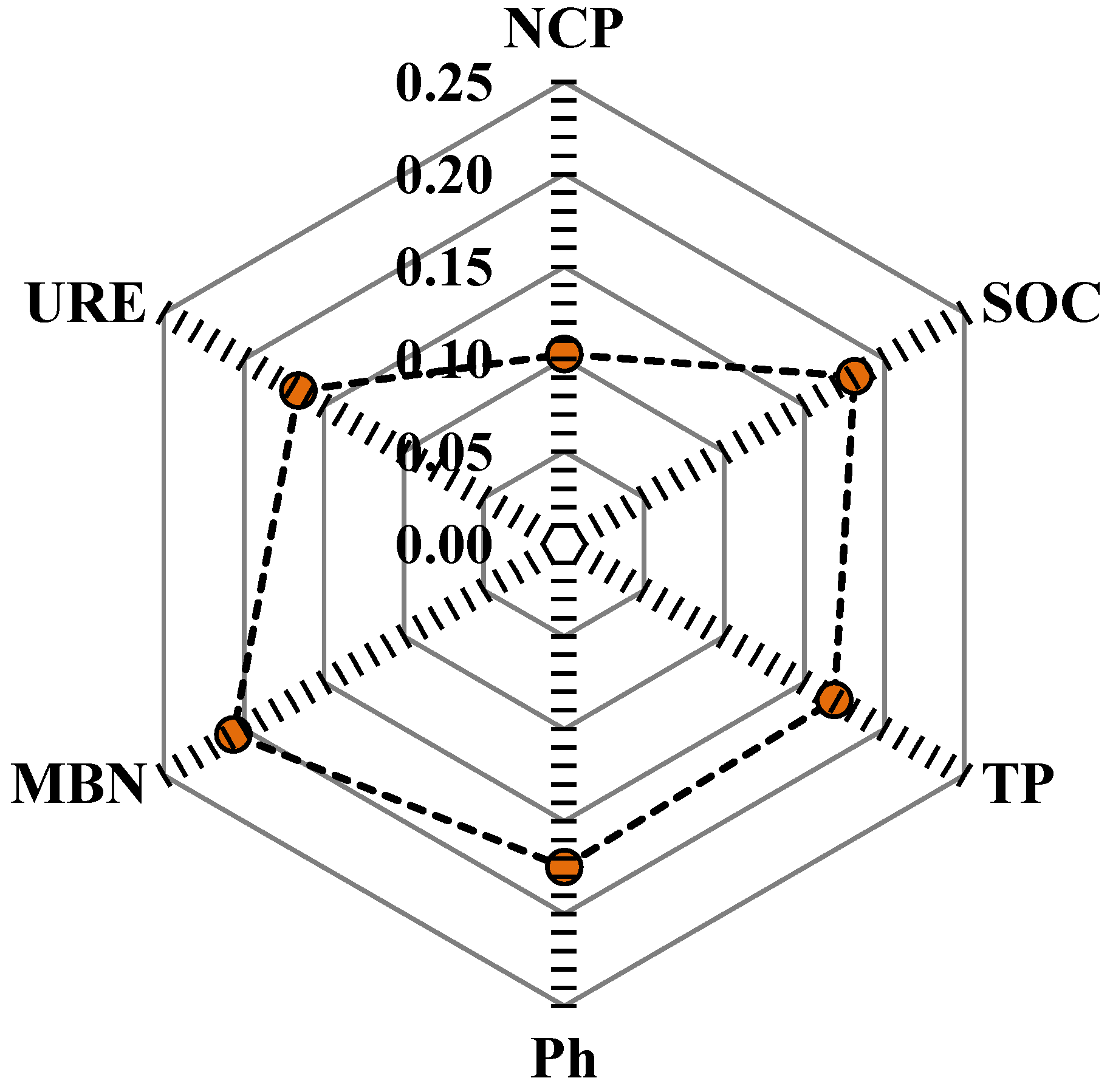
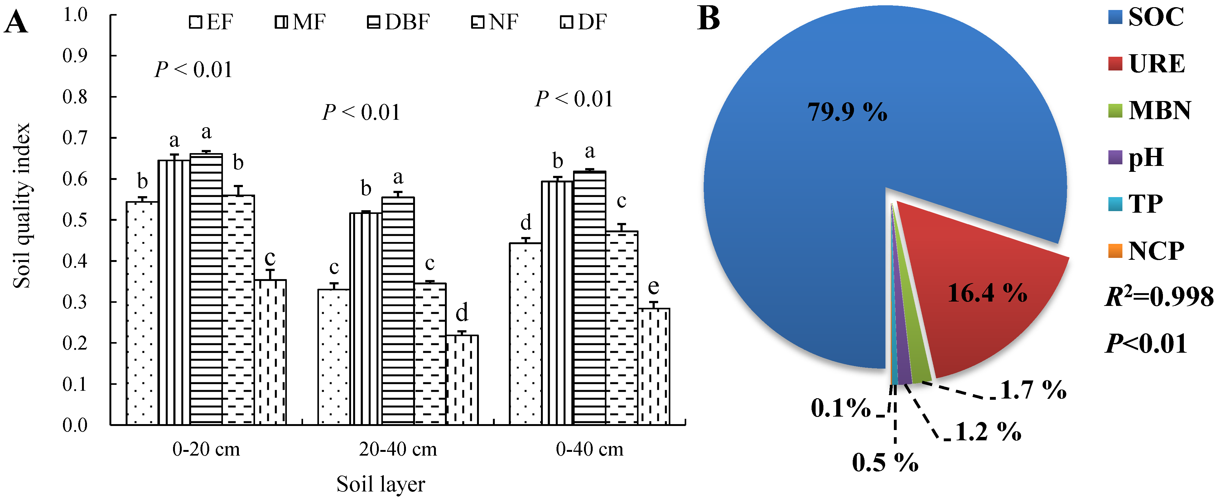
As shown in Figure 3, in all soil layers, the CAT, SAC, URE, and ALP activities exhibited significant differences between the models (p < 0.01). At 0–20 cm, the CAT activities in the MF and DBF model soils were significantly higher than the EF, NF and DF model soils, and at 20–40 cm and 0–40 cm, the activity in the DBF model was significantly higher than the EF, MF, NF, and DF models (Figure 3A). At 0–20 cm, 20–40 cm, and 0–40 cm, the soil SAC activity in the DBF model was significantly higher than the EF, MF, NF, and DF models (Figure 3B). At 0–20 cm, the soil URE activity in the MF model was significantly higher than the EF, DBF, NF, and DF models, and at 20–40 cm and 0–40 cm, the activities in the MF and DBF models were significantly higher than the EF, NF, and DF models (Figure 3C). At 0–20 cm, the soil ALP activity in the DBF model was significantly higher than the EF, MF, NF, and DF models, and at 20–40 cm and 0–40 cm, the activities in the MF and DBF models were significantly higher than the EF, NF, and DF models (Figure 3D).
Within the same model, differences in enzyme activities were significant at different soil layers. The SAC, URE, and ALP activities were reduced with an increasing soil depth in all models. This was the same for the CAT activity in only four models (EF, MF, NF, and DF), but the opposite in the DBF model.

3.4. SQI Evaluation

Factor analysis was performed on soil property indicators in the restoration models. The Kaiser–Meyer–Olkin (KMO) test was 0.712 with a p < 0.01, suggesting the PCA was appropriate. The PCA results showed that the cumulative contribution rate of the variance for the first four principal components was 95.18%, which fully explained the soil attribute information of the models (Table 4). The MBN and TK in the first principal component (PC-1) were high-weight indicators, but because the correlation between the MBN and TK was (0.880) > 0.600 (Table 5), and the weight of the MBN was >TK, only the MBN was selected to be included in the MDS. The TPO, pH, CP, MC, and SOC were indicators with a relatively high weight in the PC-2, with the pH showing the highest weight. The correlation of the TPO, CP, and MC to the pH was >0.600, but the SOC to pH was <0.600; therefore, the pH and SOC were selected for the MDS. URE, TP, and AP were the indicators with a relatively high weight in the PC-3, with the URE having the highest weight. The correlation of the AP to URE was >0.600, but the TP to URE was <0.600; therefore, the URE and TP were selected for the MDS. The NCP was the only high-weight indicator in the PC-4, so it was chosen. In total, six indicators were included in the MDS, including the NCP, SOC, TP, pH, MBN, and URE. The weight of each indicator was calculated using PCA (Figure 4), with the SQI determined as follows:
SQI = 0.10 NCP + 0.18 SOC + 0.17 TP + 0.17 pH + 0.21 MBN + 0.17 URE
Significant differences in the SQI were observed across the models (p < 0.01) (Figure 5A). At the 0–20 cm depth, the SQI order of the five models was DBF (0.661) > MF (0.645) > NF (0.560) > EF (0.544) > DF (0.353), indicating an increase of 86.9%, 82.5%, 58.5%, and 53.9% in the DBF, MF, NF, and EF models when compared with the DF model, respectively. The SQI was reduced as the soil depth increased in the models (Figure 4). At the 20–40 cm depth, DBF (0.555) > MF (0.517) > NF (0.345) > EF (0.330) > DF (0.218) was seen for the SQI, and the SQI of the DBF, MF, NF, and EF models was 154.1%, 136.5%, 58.1%, and 51.2% higher than the DF model, respectively. As a whole (0–40 cm), the overall SQI order in all of the models was DBF (0.618) > MF (0.593) > NF (0.472) > EF (0.443) > DF (0.284), and when compared with the minimum value in the DF model, the SQI was increased by 117.6%, 108.9%, 66.3%, and 55.9% in the DBF, MF, NF, and EF models, respectively.
Stepwise regression analyses showed that the SOC, URE, MBN, pH, TP, and NCP explained 79.9%, 16.4%, 1.7%, 1.2%, 0.5%, and 0.1% of the variation in the SQI (Figure 5B), suggesting the SOC was a key SQI determinant.

4. Discussion

4.1. Soil Properties in Different Models

Our results indicated significant differences in the soil physical and chemical properties in the different vegetation restoration models. We observed that these properties in the EF, MF, and DBF models, and one natural restoration model, the NF, were significantly better than the artificial disturbance model, the DF (Table 2 and Table 3), which was consistent with previous studies [21,22,23]. Thus, the artificial forest (EF, MF, and DBF) and natural restoration (NF) models could effectively improve the soil structure and nutrients in Karst rocky desertification areas. At the 0–40 cm soil layer, the MC level in the EF and MF models was significantly higher than in the DBF, NF, and DF models; the BD level in the EF, MF, and DBF models was significantly lower than in the NF and DF models; the NCP level in the NF model was significantly higher than in the EF, MF, DBF, and DF models; the CP level and TPO level in the MF model were significantly higher than in the EF, DBF, NF, and DF models (Table 2), which indicated that there were significant differences in the soil physical properties among the different models. This may have been related to the different root distribution, humus annual accumulation, and decomposition degree of different tree species in different models; however, the specific reasons require further study [21,32,33].The TP and AP levels in the MF model at a depth of 0–40 cm were the highest (Table 3), which may have been related to the organic acids secreted by the plants; when plants secrete organic acids, more oxalic acid is secreted, which effectively improves the phosphorus efficiency [34,35]. Maximum TN, TK, AN, and AK values were observed in the DBF model (Table 3), suggesting relatively high soil nutrients and fertility, possibly attributed to different biomass accumulation, distribution, litter input, and decomposition patterns [36]. More investigations are required to elucidate these underlying mechanisms.
The soil MBC and MBN are important “sources” or “sinks” of carbon and nitrogen required by vegetation [37]. They are recognized as important evaluators of soil quality or fertility, serving as early-warning and sensitive indicators of soil ecosystem changes [38]. In this study, the MBC and MBN were significantly different across the models (Figure 2A,B), suggesting the microbial biomass was substantially affected by the vegetation type, which was consistent with Peng et al. [23]. The soil MBC and MBN from three artificial models (EF, MF, and DBF) and the NF model were significantly higher than the values from the DF model, with the DBF model having the highest MBC and MBN (Figure 2A,B). Related studies showed that the soil microbial biomass was related to environmental factors such as the soil moisture, temperature, and physical and chemical soil properties [39,40].Our results showed that the MBC and MBN displayed no significant correlations with the soil moisture content and soil physical properties, but had significant positive correlations with soil nutrient indices (SOC, TN, TK, AN, and AK) (Table 5), suggesting that the soil moisture content and soil physical properties were not the main factors affecting the soil microbial biomass under the given regional climate and soil conditions, but the total amount of soil nutrients were, and their availability was significant. The TN, TK, AN, and AK in the DBF model were significantly better than the other four models (Table 3). Therefore, the highest soil MBC and MBN in the DBF model may have been due to better soil nutrients in this model [39,40].
Soil enzymes are important soil quality elements and play roles in several key chemical and material cycling processes in soil [41]. Previous studies reported that soil enzyme activity was influenced by the forest type, primarily via changes in soil physical properties caused by the mechanical actions of root systems [42]. Moreover, soil microorganism activities are directly or indirectly affected by root exudates, root litter, above-ground litter, and changes in soil microhabitats due to vegetation cover, thereby modulating the soil enzyme activity [43]. In our study, the activities of four enzymes were significantly correlated with the SOC and AN levels (Table 5). Because these levels in the DBF and MF models were substantially greater than in the EF, NF, and DF models, the activities of all four enzymes were relatively higher in the DBF and MF models (Figure 3).

4.2. The Effects of Vegetation Type on Soil Quality

Vegetation restoration improves the soil quality, but different types have various capabilities [21,23,44]. Our results showed that the soil quality (0–40 cm) of the DBF, MF, NF, and EF models was significantly higher than in the DF model, while the soil quality in the DBF and MF models was significantly higher than in the NF model (Figure 5A). These observations suggested that the soil quality of the artificial forest restoration (DBF and MF) models was higher than in the natural restoration model, and that quality in the natural restoration model was higher than in the disturbance model. Guan and Fan [22] and Pang et al. [23] also studied the soil quality of vegetation restoration in Karst areas. They indicated that the soil quality of the natural restoration model was higher than the artificial forest restoration model, in contrast to our results. This may have been due to the different tree species used in their restoration models. Guan and Fan [22] and Pang et al. [23] mainly used economic forest tree species and fast-growing introduced species to build their restoration model; these species absorbed more soil nutrients than the species in their natural restoration model because of their high yields and rapid growth; therefore, the soil quality in their natural restoration model was higher because of the limited nutrient loss. In contrast, in our study, local and native tree species were used to construct the restoration vegetation models, thereby providing robust adaptability and stress resistance in the Karst areas. Their biological characteristics increased the soil quality when compared with the natural restoration model [7]. With an increasing soil depth, the soil quality was reduced across all models (Figure 5A), consistent with previous studies [21,45]. The main reason was that litter accumulated in the surface layer and transformed into nutrients, from which the microbial activity improved the upper soil quality [21,46,47]. The soil quality of the DF model was significantly lower than that of the artificial forest restoration and NF model, mainly due to the special geological and climatic conditions in the Karst area, which has the characteristics of a small environmental capacity, a weak anti-interference ability, a low stability, and a weak self-regulation ability [48]. The destruction of vegetation by human disturbance affected the material and energy balance of the Karst soil–vegetation system, induced by the reverse evolution of the soil–vegetation system, led to the intensification of soil and water loss, and the easy loss of organic carbon in the surface soil [49]. At the same time, human disturbance caused changes in the Karst vegetation community structure and litter return quality, increased the net mineralization rate of the organic matter, and increased the risk of soil nutrient loss [50]. This series of reasons led to the serious degradation of the soil quality in the DF model.
This study showed that, among the six indices contained in the MDS, the SOC was the main index affecting the soil quality (Figure 5B). This was because the SOC is a major nutrient reservoir which not only improves the soil structure, and enhances the water permeability, water storage, and ventilation, but also increases the phosphorus and microelement availability in soils [47]. In addition, the SOC is a major source of nutrients and energy for soil microbes [22,51,52], with enzymes being the main mediators of soil biological processes, playing roles in SOC decomposition and transformation [53,54,55]. Therefore, changes in the SOC substantially affected the physical, chemical, and biological properties of the soils. Studies have shown that the conversion of land-use from agriculture to forest generally increases the soil acidity, and atmospheric deposition makes a large contribution to soil acidification [56]. However, the rate of soil acidification also depends on the specific litter quality and litter decomposition rate of the tree species [24]. In this study, soil acidification was offset by a large amount of litter input in the DBF model. Therefore, the pH value is also one of the main factors to characterize soil quality. The main direct source of phosphorus in soil is the decomposition of organic matter [56]. In this study, the MF and DBF treatments had a large amount of litter input, which significantly increased the total phosphorus content and affected the soil quality.
This study showed significant differences in the soil quality between the DBF and MF models (0–40 cm) (Figure 5A). Among the six indices contained in the MDS, no significant differences were observed in the SOC (Table 3) and URE (Figure 3C) between the DBF and MF models, but significant differences were observed for the MBN (Figure 2B), pH, TP (Table 3), and NCP, suggesting differences in the soil quality between the two models may have been due to differences in the MBN, pH, TP, and NCP. Similarly, significant differences were observed in the soil quality between the MF and EF models (0–40 cm) (Figure 5A), while no significant differences were seen in the SOC and TP between the models (Table 3), but significant differences were observed for the MBN (Figure 2B), pH (Table 3), URE (Figure 3C), and NCP, suggesting that differences in the soil quality between the two models may have arisen due to differences in the MBN, pH, URE, and NCP. Therefore, the MBN, TP, pH, URE, and NCP in the MDS were important factors affecting the soil quality (Figure 5B).

5. Conclusions

We demonstrated that vegetation types significantly influenced the soil physical and chemical properties, microbial biomass, and enzyme activities in the Karst areas of China. Of these, the MC, CP, TPO, TP, AP, and URE levels were the highest in the MF model, whereas the SOC, TN, TK, AN, AK, MBC, MBN, CAT, SAC, and ALP levels were the highest in the DBF model. Based on the MDS, six indicators, NCP, SOC, TP, pH, MBN, and URE, were selected to evaluate the soil quality across the models. Our data showed the best soil quality was in the DBF model, followed by the MF model, whereas the poorest quality was in the DF model. The SOC in the MDS explained 79.9% of the variation in the SQI, suggesting that it is a key factor affecting the soil quality.
In short, vegetation restoration models with native tree species improved the soil quality in Karst rocky desertification areas. Artificial forests (EF, MF, and DBF) performed better than natural regeneration (NF) and disturbance models (DF) in terms of restoring the soil quality. Thus, the selection of the suitable vegetation types for restoration is vitally important for the improvement in the soil quality. Moreover, this study is beneficial for implementing ecological restoration practices and management in degraded Karst areas. However, to assess the soil quality more comprehensively and precisely, the biological properties of soils should also be considered for the SQI in future studies.

Author Contributions

Conceptualization, S.-X.W.; Data curation, H.-B.O., X.-S.L. and F.G.; Formal analysis, H.-B.O., X.-S.L., S.-X.W. and Y.J.; Investigation, H.-B.O., X.-S.L., S.-X.W., Z.-H.W., W.F. and H.D.; Methodology, H.-B.O. and Y.J.; Resources, Y.J. and Y.J.; Software, H.-B.O. and Y.J.; Validation, H.-B.O. and Y.J.; Writing—original draft, H.-B.O. and Y.J.; Writing—review and editing, Y.J., X.-S.L. and S.-X.W. All authors have read and agreed to the published version of the manuscript.

Funding

The Guangxi Key R&D Program (GKAB24010090 and GKAB21220026).

Data Availability Statement

Data are contained within the article.

Acknowledgments

The authors are grateful to Hu Du, Ping-Kun Liu, Wei Bo, and Fu-Ping Zeng of the Huangjiang Observation and Research Station for Karst Ecosystems, Chinese Academy of Science, who provided facilities and constructive suggestions for this project.

Conflicts of Interest

The authors declare no conflicts of interest.

References

  1. Ding, M.M.; Yi, W.M.; Liao, L.Y.; Martens, R.; Insam, H. Effect of afforestation on microbial biomass and activity in soils of tropical China. Soil Biol. Biochem. 1992, 24, 865–872. [Google Scholar] [CrossRef]
  2. Badiane, N.N.Y.; Chotte, J.L.; Pate, E.; Masse, D.; Rouland, C. Use of soil enzymes to monitor soil quality in natural and improved fallows in semi-arid tropical regions. Appl. Soil Ecol. 2001, 18, 229–238. [Google Scholar] [CrossRef]
  3. Karlen, D.L.; Ditzler, C.A.; Andrews, S.S. Soil quality: Why and how? Geoderma 2003, 114, 145–156. [Google Scholar] [CrossRef]
  4. Zhang, W.; Zhao, J.; Pan, F.; Li, D.; Chen, H.; Wang, K. Changes in nitrogen and phosphorus limitation during secondary succession in a karst region in southwest China. Plant Soil 2015, 391, 77–91. [Google Scholar] [CrossRef]
  5. Zhao, Y.J.; Li, Z.; Zhang, J.; Song, H.Y.; Liang, Q.H.; Tao, J.P.; Cornelissen, J.H.C.; Liu, J.C. Do shallow soil, low water availability, or their combination increase the competition between grasses with different root systems in karst soil? Environ. Sci. Pollut. R. 2017, 24, 10640–10651. [Google Scholar] [CrossRef]
  6. Hu, N.; Li, H.; Tang, Z.; Li, Z.F.; Li, G.C.; Jiang, Y.; Hu, X.M.; Lou, Y.L. Community size, activity and C: N stoichiometry of soil microorganisms following reforestation in a Karst region. Eur. J. Soil Biol. 2016, 73, 77–83. [Google Scholar] [CrossRef]
  7. Pedraza, R.A.; Williams-Linera, G. Evaluation of native tree species for the rehabilitation of deforested areas in a Mexican cloud forest. New For. 2003, 26, 83–99. [Google Scholar] [CrossRef]
  8. Diemont, S.A.W.; Martin, J.F.; Levy-Tacher, S.I.; Nigh, R.B.; Lopez, P.R.; Golicher, J.D. Lacandon Maya forest management: Restoration of soil fertility using native tree species. Ecol. Eng. 2006, 28, 205–212. [Google Scholar] [CrossRef]
  9. Deng, L.; Liu, G.B.; Shangguan, Z.P. Land-use conversion and changing soil carbon stocks in China’s ‘Grain-for-Green’ program: A synthesis. Glob. Change Biol. 2015, 20, 3544–3556. [Google Scholar] [CrossRef]
  10. Homolák, M.; Kriaková, E.; Pichler, V.; Gömöryová, E.; Bebej, J. Isolating the soil type effect on the organic carbon content in a Rendzic Leptosol and an Andosol on a limestone plateau with andesite protrusions. Geoderma 2017, 302, 1–5. [Google Scholar] [CrossRef]
  11. Chang, J.; Zhu, J.; Xu, L.; Su, H.; Gao, Y.; Cai, X.; Peng, T.; Wen, X.; Zhang, J.; He, N. Rational land-use types in the karst regions of China: Insights from soil organic matter composition and stability. Catena 2018, 160, 345–353. [Google Scholar] [CrossRef]
  12. Li, D.; Zhang, X.; Green, S.M.; Dungait, J.A.J.; Wen, X.; Tang, Y.; Guo, Z.; Yang, Y.; Sun, X.; Quine, T.A. Nitrogen functional gene activity in soil profiles under pro-gressive vegetative recovery after abandonment of agriculture at the Puding Karst Critical Zone Observatory, SW China. Soil Biol. Biochem. 2018, 125, 93–102. [Google Scholar] [CrossRef]
  13. Lan, J.; Hu, N.; Fu, W. Soil carbon–nitrogen coupled accumulation following the natural vegetation restoration of abandoned farmlands in a karst rocky desertification region. Ecol. Eng. 2020, 158, 106033. [Google Scholar] [CrossRef]
  14. Garousi, F.; Shan, Z.; Ni, K.; Yang, H.; Shan, J.; Cao, J.; Jiang, Z.; Yang, J.; Zhu, T.; Müller, C. Decreased inorganic N supply capacity and turnover in calcareous soil under degraded rubber plantation in the tropical karst region. Geoderma 2021, 381, 114754. [Google Scholar] [CrossRef]
  15. Raiesi, F.; Beheshti, A. Soil C turnover, microbial biomass and respiration, and enzymatic activities following rangeland conversion to wheat–alfalfa cropping in a semi-arid climate. Environ. Earth Sci. 2014, 72, 5073–5088. [Google Scholar] [CrossRef]
  16. Fu, T.; Chen, H.; Zhang, W.; Nie, Y.; Gao, P.; Wang, K. Spatial variability of surface soil saturated hydraulic conductivity in a small karst catchment of southwest China. Environ. Earth Sci. 2015, 74, 2381–2391. [Google Scholar] [CrossRef]
  17. Pan, F.; Zhang, W.; Liu, S.; Li, D.; Wang, K. Leaf N:P stoichiometry across plant functional groups in the karst region of southwestern China. Trees 2015, 29, 883–892. [Google Scholar] [CrossRef]
  18. Knáb, M.; Szili-Kovács, T.; Kiss, K.; Palatinszky, M.; Márialigeti, K.; Móga, J.; Borsodi, A. Comparison of soil microbial communities from two distinct karst areas in Hungary. Acta Microbiol. Imm. H. 2012, 59, 91–105. [Google Scholar] [CrossRef]
  19. Zhao, C.; Long, J.; Liao, H.; Zheng, C.; Li, J.; Liu, L.; Zhang, M. Dynamics of soil microbial communities following vegetation succession in a karst mountain ecosystem, Southwest China. Sci. Rep. 2019, 9, 2160. [Google Scholar] [CrossRef]
  20. Hu, P.; Xiao, J.; Zhang, W.; Xiao, L.; Yang, R.; Xiao, D.; Zhao, J.; Wang, K. Response of soil microbial communities to natural and managed vegetation restoration in a subtropical karst region. Catena 2020, 195, 104849. [Google Scholar] [CrossRef]
  21. Zhang, Y.; Xu, X.; Li, Z.; Liu, M.; Xu, C.; Zhang, R.; Luo, W. Effects of vegetation restoration on soil quality in degraded karst landscapes of southwest China. Sci. Total Environ. 2019, 650, 2657–2665. [Google Scholar] [CrossRef]
  22. Guan, H.; Fan, J. Effects of vegetation restoration on soil quality in fragile karst ecosystems of southwest China. PeerJ 2020, 8, e9456. [Google Scholar] [CrossRef]
  23. Pang, D.; Cao, J.; Dan, X.; Guan, Y.; Peng, X.; Cui, M.; Wu, X.; Zhou, J. Recovery approach affects soil quality in fragile karst ecosystems of southwest China: Implications for vegetation restoration. Ecol. Eng. 2018, 123, 151–160. [Google Scholar] [CrossRef]
  24. Lu, Z.X.; Wang, P.; Ou, H.B.; Wei, S.X.; Wu, L.C.; Jiang, Y. Effects of different vegetation restoration on soil nutrients, enzyme activities, and microbial communities in degraded karst landscapes in southwest China. For. Ecol. Manag. 2022, 508, 120002. [Google Scholar] [CrossRef]
  25. Liu, G. Soil Physical and Chemical Analysis & Description of Soil Profiles; Standards Press of China: Beijing, China, 1996; pp. 5–19. [Google Scholar]
  26. Lu, R.K. Analysis Methods of Soil Agricultural Chemistry; China Agricultural Science and Technology Press: Beijing, China, 1999; pp. 474–490. [Google Scholar]
  27. Huang, C.; Zeng, Y.; Wang, L.; Wang, S. Responses of soil nutrients to vegetation restoration in China. Reg. Environ. Change 2020, 20, 82. [Google Scholar] [CrossRef]
  28. Wu, J.; Joergensen, R.G.; Pommerening, B.; Chaussod, R.; Brookes, P.C. Measurement of soil microbial biomass C by fumigation-extraction-an automated procedure. Soil Biol. Biochem. 1990, 22, 1167–1169. [Google Scholar] [CrossRef]
  29. Iqbal, J.; Hu, R.; Feng, M.; Lin, S.; Malghani, S.; Ali, I.M. Microbial biomass, and dissolved organic carbon and nitrogen strongly affect soil respiration in different land uses: A case study at Three Gorges Reservoir Area, South China. Agr. Ecosyst. Environ. 2010, 137, 294–307. [Google Scholar] [CrossRef]
  30. Sanchez-Hernandez, J.C.; Notario del Pino, J.; Capowiez, Y.; Mazzia, C.; Rault, M. Soil enzyme dynamics in chlorpyrifos-treated soils under the influence of earthworms. Sci. Total Environ. 2018, 612, 1407–1416. [Google Scholar] [CrossRef]
  31. Andrews, S.S.; Karlen, D.L.; Cambardella, C.A. The soil management assessment framework: A quantitative soil quality evaluation method. Soil Sci. Soc. Am. J. 2004, 68, 1945–1962. [Google Scholar] [CrossRef]
  32. Danise, T.; Andriuzzi, W.S.; Battipaglia, G.; Certini, G.; Guggenberger, G.; Innangi, M.; Mastrolonardo, G.; Niccoli, F.; Pelleri, F.; Fioretto, A. Mixed-species plantation effects on soil biological and chemical quality and tree growth of a former agricultural land. Forests 2021, 12, 842. [Google Scholar] [CrossRef]
  33. Chen, Y.L.; Zhang, Z.S.; Huang, L.; Zhao, Y.; Hu, Y.G.; Zhang, P.; Zhang, D.H.; Zhang, H. Co-variation of fine-root distribution with vegetation and soil properties along a revegetation chronosequence in a desert area in northwestern China. Catena 2017, 151, 16–25. [Google Scholar] [CrossRef]
  34. Ström, L.; Owen, A.; Godbold, D.; Jones, D. Organic acid behaviour in a calcareous soil: Sorption reactions and biodegradation rates. Soil Biol. Biochem. 2001, 33, 2125–2133. [Google Scholar] [CrossRef]
  35. Clarholm, M.; Skyllberg, U.; Rosling, A. Organic acid induced release of nutrients from metal-stabilized soil organic matter—The unbutton model. Soil Biol. Biochem. 2015, 84, 168–176. [Google Scholar] [CrossRef]
  36. Zhang, K.; Dang, H.; Tan, S.; Wang, Z.; Zhang, Q. Vegetation community and soil characteristics of abandoned agricultural land and pine plantation in the Qinling Mountains, China. For. Ecol. Manag. 2010, 259, 2036–2047. [Google Scholar] [CrossRef]
  37. Friedel, J.K.; Munch, J.C.; Fischer, W.R. Soil microbial properties and the assessment of available soil organic matter in a haplic Luvisol after several years of different cultivation and crop rotation. Soil Biol. Biochem. 1996, 28, 479–488. [Google Scholar] [CrossRef]
  38. Pignataro, A.; Moscatelli, M.C.; Mocali, S.; Grego, S.; Benedetti, A. Assessment of soil microbial functional diversity in a coppiced forest system. Appl. Soil Ecol. 2012, 62, 115–123. [Google Scholar] [CrossRef]
  39. Xu, X.; Yin, L.; Duan, C.; Jing, Y. Effect of N addition, moisture, and temperature on soil microbial respiration and microbial biomass in forest soil at different stages of litter decomposition. J. Soil Sediment. 2016, 16, 1421–1439. [Google Scholar] [CrossRef]
  40. Song, P.; Ren, H.; Jia, Q.; Guo, J.; Zhang, N.; Ma, K. Effects of historical logging on soil microbial communities in a subtropical forest in southern China. Plant Soil 2015, 397, 115–126. [Google Scholar] [CrossRef]
  41. Udawatta, R.P.; Kremer, R.J.; Garrett, H.E.; Anderson, S.H. Soil enzyme activities and physical properties in a watershed managed under agroforestry and row-crop systems. Agric. Ecosyst. Environ. 2009, 131, 98–104. [Google Scholar] [CrossRef]
  42. Acosta-Martínez, V.; Cruz, L.; Sotomayor-Ramírez, D.; Pérez-Alegría, L. Enzyme activities as affected by soil properties and land use in a tropical watershed. Appl. Soil Ecol. 2007, 35, 35–45. [Google Scholar] [CrossRef]
  43. Hao, Y.; Chang, Q.; Li, L.; Wei, X. Impacts of landform, land use and soil type on soil chemical properties and enzymatic activities in a Loessial Gully watershed. Soil Res. 2014, 52, 453. [Google Scholar] [CrossRef]
  44. Marzaioli, R.; D’Ascoli, R.; Pascale, R.A.D.; Rutigliano, F.A. Soil quality in a Mediterra-nean area of southern Italy as related to different land use types. Appl. Soil Ecol. 2010, 44, 205–212. [Google Scholar] [CrossRef]
  45. Guo, S.; Han, X.; Li, H.; Wang, T.; Tong, X.; Ren, G.; Feng, Y.; Yang, G. Evaluation of soil quality along two revegetation chronosequences on the Loess Hilly Region of China. Sci. Total Environ. 2018, 633, 808–815. [Google Scholar] [CrossRef]
  46. Zhang, Z.; Yu, X.; Qian, S.; Li, J. Spatial variability of soil nitrogen and phosphorus of a mixed forest ecosystem in Beijing, China. Environ. Earth Sci. 2009, 60, 1783–1792. [Google Scholar] [CrossRef]
  47. Mukhopadhyay, S.; Masto, R.E.; Yadav, A.; George, J.; Ram, L.C.; Shukla, S.P. Soil quality index for evaluation of reclaimed coal mine spoil. Sci. Total Environ. 2016, 542, 540–550. [Google Scholar] [CrossRef]
  48. Chen, H.S.; Wang, K.L. Characteristics of karst drought and its countermeasures. Res. Agric. Mod. 2004, 25, 70–73. (In Chinese) [Google Scholar]
  49. Chen, H.S.; Zhang, W.; Wang, K.L.; Hou, Y. Soil organic carbon and total nitrogen as affected by land use types in karst and non-karst areas of northwest Guangxi, China. J. Sci. Food Agric. 2012, 92, 1086–1093. [Google Scholar] [CrossRef]
  50. Liu, S.J.; Zhang, W.; Wang, K.L.; Pan, F.; Yang, S.; Shu, S. Factors controlling accumulation of soil organic carbon along vegetation succession in a typical karst region in Southwest China. Sci. Total Environ. 2015, 521, 52–58. [Google Scholar] [CrossRef]
  51. Bhogal, A.; Nicholson, F.A.; Chambers, B.J. Organic carbon additions: Effects on soil bio-physical and physico-chemical properties. Eur. J. Soil Sci. 2009, 60, 276–286. [Google Scholar] [CrossRef]
  52. Cao, Y.; Wang, X.; Lu, X.; Yan, Y.; Fan, J. Soil organic carbon and nutrients along an alpine grassland transect across Northern Tibet. J. Mt. Sci. 2013, 10, 564–573. [Google Scholar] [CrossRef]
  53. Wu, Y.; Wang, F.; Zhu, S. Vertical distribution characteristics of soil organic carbon content in Caohai wetland ecosystem of Guizhou plateau, China. J. For. Res. 2015, 7, 551–556. [Google Scholar] [CrossRef]
  54. Xiao, Y.; Huang, Z.; Lu, X. Changes of soil labile organic carbon fractions and their relation to soil microbial characteristics in four typical wetlands of Sanjiang Plain, Northeast China. Ecol. Eng. 2015, 82, 381–389. [Google Scholar] [CrossRef]
  55. Yan, Y.; Dai, Q.; Wang, X.; Jin, L.; Mei, L. Response of shallow karst fissure soil quality to secondary succession in a degraded karst area of southwestern China. Geoderma 2019, 348, 76–85. [Google Scholar] [CrossRef]
  56. Reich, P.B.; Oleksyn, J.; Modrzynski, J.; Mrozinski, P.; Hobbie, S.E.; Eissenstat, D.M.; Chorover, J.; Chadwick, O.A.; Hale, C.M.; Joelker, M.G. Linking litter calcium, earthworms and soil properties: A common garden test with 14 tree species. Ecol. Lett. 2005, 8, 811–818. [Google Scholar] [CrossRef]
Figure 1. Location of the study area at the Huanjiang Observation and Research Station for Karst Ecosystems of the Chinese Academy of Sciences (CAS), Guangxi province, Southwest China.
Forests 15 01061 g001
Figure 2. Soil microbial biomass C (A) and N (B) in restoration models at different soil depths. EF, evergreen broad-leaved forest; MF, mixed forest; DBF, deciduous broad-leaved forest; NF, natural closed forest; DF, disturbed forest. Significant differences (p < 0.01 using Duncan’s new multiple-range test) are indicated by different letters.
Forests 15 01061 g002
Figure 3. Soil enzyme activities in models at different soil depths: (A) catalase (CAT) activity, (B) sucrose (SAC) activity, (C) urease (URE) activity, and (D) alkaline phosphatase (ALP) activity. EF, evergreen broad-leaved forest; MF, mixed forest; DBF, deciduous broad-leaved forest; NF, natural closed forest; DF, disturbed forest. Significant differences (p < 0.01 using Duncan’s new multiple-range test) are indicated by different letters.
Forests 15 01061 g003aForests 15 01061 g003b
Figure 4. Soil parameter weights from the MDS. NCP, non-capillary porosity; SOC, soil organic carbon; TP, total phosphorus; MBN, soil microbial biomass N; URE, urease activity.
Forests 15 01061 g004
Figure 5. Soil quality index (SQI) in different models (A) and the contribution rate of selected indicators in determining the SQI using the minimum data set (MDS) method (B). EF, evergreen broad-leaved forest; MF, mixed forest; DBF, deciduous broad-leaved forest; NF, natural closed forest; DF, disturbed forest; SOC, soil organic carbon; URE, urease activity; MBN, soil microbial biomass N; TP, total phosphorus; NCP, non-capillary porosity; Significant differences (p < 0.01 using Duncan’s new multiple-range test) are indicated by different letters.
Forests 15 01061 g005
Table 1. Basic profiles of the experimental plots.
Site CharacteristicsEvergreen Broad-Leaved Forest (EF)Mixed Forest (MF)Deciduous Broad-Leaved Forest (DBF)Natural Closed Forest (NF)Disturbed Forest (DF)
Test area (hm2)0.280.290.230.140.15
Elevation (m)286–337288–337287–337291–339294–340
Slope (°)2424243335
AspectSoutheastSoutheastSoutheastSoutheastSoutheast
Soil typeCalcareousCalcareous Calcareous Calcareous Calcareous
TreatmentCut down a small part of the original vegetation for planting evergreen treesCut down a small part of the original vegetation for planting evergreen and deciduous treesCut down a small part of the original vegetation for planting deciduous treesPreserve the original vegetationAll shrubs and herbs were regularly cut down every year without removing underground roots
Recovery time (year)1313131313
Mean tree height (m)9.19.212.13.5
Mean diameter at BREAST Height (cm)8.48.913.23.2
Vegetation cover (%)60706085
Mean density (Plant/hm2)91311501450
Thickness of humus layer/cm1–33–45–64–50–1
Soil thickness/cm40–6040–6040–6050–7040–60
Main speciesC. glauca,
Rhus chinensis Mill, Jasminum nervosum Lour.,
Ficus tikoua Bur.,
Microstegium fasciculatum (L.) Henrard,
Cyclosorus parasiticus (L.) Farw.
C. axillaris,
Delavaya toxocarpa Franch, Z. insignis,
C. glauca,
Vitex neguwndo Linn.,
Mallotus barbatus,
J. nervosum,
C. Parasiticus,
M. fasciculatum
Z. insignis,
C. axillaris,
J. nervosum,
Leucaena leucocephala (Lam.) de Wit,
M. fasciculatum,
Miscanthus floridulus (Lab.) Warb. ex Schum. et Laut.
V. negundo,
Mallotus barbatus (Wall.) Muell. Arg.,
M. fasciculatum,
Oplismenus undulatifolius (Ard.) Roem. & Schult.
V. negundo,
Dalbergia balansae Prain,
M. fasciculatum,
Imperata cylindrica (L.) Raeusch.
Note: — index not measured.
Table 2. Soil physical properties in the models (mean ± standard deviation (SD)).
IndexSoil layerEFMFDBFNFDFF
MC (%)0–20 cm34.24 ± 2.11a36.18 ± 3.43a26.35 ± 1.27b22.37 ± 2.86c20.43 ± 1.59c43.291 **
20–40 cm25.86 ± 2.01ab28.17 ± 1.35a25.10 ± 2.18b19.95 ± 0.20c19.17 ± 3.53c16.517 **
0–40 cm30.05 ± 1.49a32.18 ± 1.36a25.72 ± 1.56b21.15 ± 1.45c19.80 ± 2.15c54.959 **
BD (g/cm3)0–20 cm0.88 ± 0.19b0.81 ± 0.06b0.85 ± 0.18b1.10 ± 0.04a1.15 ± 0.03a8.388 **
20–40 cm1.01 ± 0.07bc0.91 ± 0.25c0.97 ± 0.04c1.24 ± 0.16c1.21 ± 0.17ab4.472 **
0–40 cm0.95 ± 0.13b0.86 ± 0.15b0.92 ± 0.10b1.17 ± 0.10a1.18 ± 0.07a8.848 **
NCP (%)0–20 cm5.41 ± 0.35cd5.25 ± 0.41d5.81 ± 0.14c8.90 ± 0.58a8.09 ± 0.26b98.364 **
20–40 cm6.82 ± 0.10b7.11 ± 0.35b3.72 ± 0.14d7.89 ± 0.34a6.42 ± 0.19c209.944 **
0–40 cm6.09 ± 0.19c6.18 ± 0.19c4.77 ± 0.13d8.40 ± 0.43a7.26 ± 0.22b143.891 **
CP (%)0–20 cm53.12 ± 1.36b57.81 ± 0.68a41.02 ± 0.97c35.08 ± 0.61d25.03 ± 0.75e1057.997 **
20–40 cm42.79 ± 0.72b47.09 ± 1.04a40.48 ± 0.57c33.91 ± 2.14d20.02 ± 0.44e414.490 **
0–40 cm48.47 ± 1.16b52.45 ± 0.76a40.75 ± 0.55c34.49 ± 1.21d22.53 ± 0.53e882.855 **
TPO (%)0–20 cm58.53 ± 1.18b63.06 ± 1.22a46.84 ± 1.00c43.98 ± 1.06d33.12 ± 1.63e465.011 **
20–40 cm49.61 ± 1.05b54.20 ± 1.18a44.20 ± 0.34c41.80 ± 1.35d26.44 ± 0.90e532.092 **
0–40 cm54.36 ± 1.02b58.63 ± 0.58a45.52 ± 0.48c42.89 ± 0.84d29.78 ± 1.11e885.410 **
Footnote: EF, evergreen broad-leaved forest; MF, mixed forest; DBF, deciduous broad-leaved forest; NF, natural closed forest; DF, disturbed forest; MC, soil moisture content; BD, soil bulk density; NCP, non-capillary porosity; CP, capillary porosity; TPO, total porosity. Different lowercase letters in the same line show significant differences at the p = 0.05 level; ** significant at the 0.01 probability level.
Table 3. Soil chemical properties in the models (mean ± standard deviation (SD)).
IndexSoil LayerEFMFDBFNFDFF
SOC (g/kg)0–20 cm88.11 ± 2.84a89.94 ± 2.78a90.39 ± 0.12a88.29 ± 2.46a73.68 ± 2.33b45.006 **
20–40 cm69.06 ± 1.78bc74.16 ± 2.57a71.04 ± 1.13b67.74 ± 0.83c39.09 ± 2.37d292.465 **
0–40 cm76.69 ± 3.27b82.05 ± 1.84a80.72 ± 0.59a78.02 ± 1.51b56.39 ± 1.86c136.373 **
TN (g/kg)0–20 cm5.10 ± 0.06a5.11 ± 0.11a5.26 ± 0.09a4.56 ± 0.28b4.34 ± 0.28b22.600 **
20–40 cm3.42 ± 0.07b3.57 ± 0.20ab3.81 ± 0.28a3.39 ± 0.22b1.14 ± 0.03c171.715 **
0–40 cm4.22 ± 0.09b4.34 ± 0.11b4.54 ± 0.12a3.98 ± 0.17c2.75 ± 0.13d154.910 **
TK (g/kg)0–20 cm4.23 ± 0.08c5.79 ± 0.16b6.35 ± 0.11a5.71 ± 0.14b3.96 ± 0.17d289.145 **
20–40 cm2.62 ± 0.10c3.67 ± 0.09b4.23 ± 0.09a3.85 ± 0.11b2.33 ± 0.27d154.723 **
0–40 cm3.40 ± 0.08c4.73 ± 0.13b5.29 ± 0.10a4.78 ± 0.06b3.15 ± 0.14d423.276 **
TP (g/kg)0–20 cm1.13 ± 0.15b1.57 ± 0.26a1.15 ± 0.02b1.01 ± 0.20b1.08 ± 0.14b8.313 **
20–40 cm0.71 ± 0.03c0.90 ± 0.05a0.84 ± 0.17ab0.74 ± 0.04bc0.67 ± 0.05c6.659 **
0–40 cm0.98 ± 0.12b1.24 ± 0.14a0.99 ± 0.09b0.88 ± 0.10b0.87 ± 0.07b10.052 **
AN (mg/kg)0–20 cm256.33 ± 3.61d274.13 ± 1.43b354.53 ± 1.82a263.20 ± 2.22c252.90 ± 6.43d692.814 **
20–40 cm160.27 ± 1.59d180.20 ± 1.4b188.53 ± 3.65a168.8 ± 3.45c154.10 ± 2.41e140.017 **
0–40 cm208.30 ± 1.66d227.17 ± 0.37b271.53 ± 2.20a216.00 ± 2.72c203.50 ± 4.28e558.075 **
AP (mg/kg)0–20 cm4.00 ± 0.31c9.13 ± 0.26a6.79 ± 0.17b3.36 ± 0.12d2.32 ± 0.25e721.685 **
20–40 cm2.17 ± 0.19b4.51 ± 0.32a4.31 ± 0.10a1.84 ± 0.06c1.59 ± 0.07d317.125 **
0–40 cm2.90 ± 0.47c6.83 ± 0.16a5.55 ± 0.11b2.60 ± 0.07c1.95 ± 0.14d388.917 **
AK (mg/kg)0–20 cm153.74 ± 1.83d160.75 ± 0.68c243.33 ± 1.93a167.48 ± 1.13b135.04 ± 2.61e2773.203 **
20–40 cm108.27 ± 2.46c112.79 ± 1.7b139.49 ± 3.85a109.05 ± 3.16c89.08 ± 1.36d228.543 **
0–40 cm129.52 ± 2.37c136.77 ± 1.03b191.42 ± 2.55a138.27 ± 2.03b112.06 ± 1.94d1046.522 **
pH0–20 cm6.59 ± 0.07b6.66 ± 0.13b7.57 ± 0.18a7.72 ± 0.07a7.60 ± 0.20a2773.203 **
20–40 cm7.08 ± 0.11b6.94 ± 0.15b7.63 ± 0.14a7.74 ± 0.13a7.73 ± 0.08a48.939 **
0–40 cm6.84 ± 0.06b6.80 ± 0.09b7.60 ± 0.15a7.73 ± 0.09a7.67 ± 0.14a89.008 **
Footnote: EF, evergreen broad-leaved forest; MF, mixed forest; DBF, deciduous broad-leaved forest; NF, natural closed forest; DF, disturbed forest; SOC, soil organic carbon; TN, total nitrogen; TP, total phosphorus; TK, total potassium; AN, available nitrogen; AP, available phosphorus; AK, available potassium. Different lowercase letters in the same line show significant differences at the p = 0.05 level; ** significant at the 0.01 probability level.
Table 4. Principal component analysis of the soil quality indicators.
Principal ComponentPC-1PC-2PC-3PC-4
Eigenvalues12.0713.5831.441.044
Variance (%)63.2518.867.585.49
Cumulative (%)63.2582.1189.6995.18
MC0.0620.9000.2890.207
BD−0.188−0.606−0.088−0.572
NCP−0.143−0.302−0.203−0.896
CP0.3240.9110.1910.133
TPO0.3260.9220.1840.031
SOC0.7850.8770.1620.044
TN0.7480.5880.1180.222
TK0.879−0.0270.4440.089
TP0.0000.5870.7310.018
AN0.668−0.1160.3580.631
AP0.3750.4320.7120.343
AK0.780−0.0880.1890.568
pH0.227−0.944−0.103−0.098
MBC0.7800.0830.5690.193
MBN0.9680.1440.0540.155
CAT0.5410.1920.5050.567
SAC0.7160.6020.1510.303
URE0.5000.2230.7390.325
ALP0.5270.2620.6420.475
Note: PC-1, PC-2, PC-3, and PC-4 are the four principal components. Bold numbers are considered highly weighted. MC, soil moisture content; BD, soil bulk density; NCP, non-capillary porosity; CP, capillary porosity; TPO, total porosity; SOC, soil organic carbon; TN, total nitrogen; TP, total phosphorus; TK, total potassium; AN, available nitrogen; AP, available phosphorus; AK, available potassium; MBC, soil microbial biomass C; MBN, soil microbial biomass N; CAT, catalase activity; SAC, sucrose activity; URE, urease activity; ALP, alkaline phosphatase activity.
Table 5. Correlation analysis of the soil physical, chemical, and biotic properties.
IndexMCBDNCPCPTPOSOCTNTKTPANAPAKpHMBCMBNCATSACURE
BD−0.65 **1.00
NCP−0.53 **0.65 **1.00
CP0.92 **−0.68 **−0.491.00
TPO0.91 **−0.64 **−0.400.99 **1.00
SOC0.62 **−0.54 **−0.36 0.81 **0.82 **1.00
TN0.67 **−0.59 **−0.53 **0.83 **0.81 *0.95 **1.00
TK0.16 −0.30 −0.27 0.35 0.34 0.75 **0.70 **1.00
TP0.76 **−0.36 −0.37 0.68 **0.67 **0.440.470.29 1.00
AN0.19 −0.41−0.70 **0.26 0.20 0.54 **0.62 **0.80 **0.22 1.00
AP0.67 **−0.65 **−0.62 **0.70 **0.66 **0.68 **0.68 **0.68 **0.72 **0.66 **1.00
AK0.16 −0.38 −0.65 **0.29 0.23 0.61 **0.70 **0.81 **0.14 0.97 **0.57 **1.00
pH−0.87 **0.59 **0.36 −0.82 **−0.82 **−0.39 −0.400.16 −0.61 **0.16 −0.440.19 1.00
MBC0.31 −0.42−0.410.460.440.76 **0.73 **0.97 **0.410.83 **0.82 **0.80 **0.01 1.00
MBN0.24 −0.33 −0.34 0.480.460.85 **0.85 **0.88 **0.16 0.76 **0.50 *0.85 **0.06 0.82 **1.00
CAT0.48−0.53 **−0.75 **0.52 **0.460.65 **0.70 **0.74 **0.52 **0.89 **0.80 **0.82 **−0.18 0.81 **0.68 **1.00
SAC0.70 **−0.67 **−0.59 **0.85 **0.83 **0.94 **0.97 **0.71 **0.470.66 **0.73 **0.71 **−0.450.75 **0.84 **0.76 **1.00
URE0.50 *−0.52 **−0.57 **0.55 **0.52 **0.66 **0.65 **0.80 **0.52 **0.77 **0.95 **0.67 **−0.21 0.91 **0.59 **0.84 **0.70 **1.00
ALP0.58 **−0.59 **−0.72 **0.61 **0.56 **0.71 **0.74 **0.77 **0.62 **0.85 **0.93 **0.78 **−0.25 0.87 **0.65 **0.92 **0.78 **0.95 **
Footnote: MC, soil moisture content; BD, soil bulk density; NCP, non-capillary porosity; CP, capillary porosity; TPO, total porosity; SOC, soil organic carbon; TN, total nitrogen; TP, total phosphorus; TK, total potassium; AN, available nitrogen; AP, available phosphorus; AK, available potassium; MBC, soil microbial biomass C; MBN, soil microbial biomass N; CAT, catalase activity; SAC, sucrose activity; URE, urease activity; ALP, alkaline phosphatase activity. * and ** indicate significance at the 0.05 and 0.01 probability levels, respectively.
Disclaimer/Publisher’s Note: The statements, opinions and data contained in all publications are solely those of the individual author(s) and contributor(s) and not of MDPI and/or the editor(s). MDPI and/or the editor(s) disclaim responsibility for any injury to people or property resulting from any ideas, methods, instructions or products referred to in the content.

