Abstract
Korean pine is one of the most important tree species in northeastern China, where Korean pine plantations produce timber and edible seeds. Often, seeds create more income than timber. Predicting the timber and cone yields of alternative management schedules of the plantations involves uncertainty because the future climatic conditions for tree growth and cone production are unknown. This study developed a simulation model that generates stochastic variation around the predictions of tree growth and cone yield models, allowing the forest manager to seek cutting schedules that maximize the expected amounts of timber or cones, or the expected economic profit, under uncertain future states of nature. Stochastic analysis also facilitates management optimizations for different risk attitudes. The differential evolution algorithm and the developed stochastic simulation model were used to optimize the management of planted Korean pine. Timber and cone yields of a management schedule were calculated under 100 different scenarios for tree growth and cone production. When the growth and cone yield scenarios were stationary (no temporal trends), the optimal management schedules were similar to those of deterministic optimization. The benefits of stochastic optimization increased when it was assumed that the tree growth scenarios may contain climate-change-induced trends. Non-stationary growth variation led to shorter optimal rotation lengths than stationary growth variation. Increasing risk tolerance shortened optimal rotations.
1. Introduction
Korean pine (Pinus koraiensis Siebold & Zucc.) is one of the major tree species in the northeastern regions of China, with high ecological and economic value [1]. It occurs also in Russia, Japan, and Korea. Korean pine produces timber and edible seeds for human consumption. Other pine nut species include P. pinea, P. gerardiana, P. sibirica, and P. cembra. However, most of the marketed edible “pine nuts” sold in the world are collected from Korean pine stands [2,3].
Korean pine stands can be used for timber or seed production, or combined production of timber and seeds. If economic profit is maximized, the logical option is combined production where the relative weights of timber and cones in management decisions depend on the selling prices and production costs of these two products.
Forest planning and management optimization aim at finding the best possible future treatments for a stand or a forest [4,5]. Calculations performed in management optimization always involve uncertainty because the future growth and seed production of the trees are unknown. Seed production in particular varies a lot annually, and also in the longer term [6,7]. Future timber and seed prices are also unknown, as well as future regulations of forest management.
Previous literature reports optimization results for Korean pine when timber yield, seed production, and carbon storage are maximized [8]. Pasalodos-Tato et al. [9] optimized the management of Pinus pinea stands in the joint production of timber and pine nuts. These optimizations were conducted deterministically, i.e., assuming that the trees grow as the growth models predict and that the cone yields are equal to the predictions of the cone yield model. The fact that cone production is concentrated in a few years and these years into a few trees has been ignored in previous calculations [7,8].
In addition, previous studies assumed that one kilogram of pinecones or seeds always produces the same net income. However, since cone collection involves fixed costs, both at the stand and the tree level, the harvesting cost per cone is lower in a good seed year and higher in a bad seed year. In a bad year, the cone harvesting cost may even be higher than the selling price of the cones.
For the above reasons, a certain management scenario may produce different outcomes, depending on the future conditions for growth and seed production, and prices of timber and pinecones. This situation can be dealt with by using stochastic optimization in management planning. The so-called anticipatory approach to stochastic optimization calculates several possible outcomes for all those management schedules evaluated during the optimization process [10]. In these repeated simulations, uncertain processes such as tree growth and cone yield are assumed to be stochastic. Stochastic results are obtained by adding random variation around the predictions of tree growth and cone production models.
In this type of anticipatory stochastic optimization, each management schedule is described by the distribution of net present values, timber yields, cone yields, etc. The distributions give information about the possible ranges of the management objectives if a certain management schedule is implemented in an uncertain environment. The distributions also show the likelihood of reaching certain timber or seed production targets.
Stochastic optimization may maximize the mean value of the distribution of net present values (or any other objective variable), obtained from repeated stochastic simulations (the expected value). Maximizing the expected value corresponds to risk neutrality [11,12]. If there is a production or harvest volume target, stochastic optimization allows one to maximize the probability that the target is reached [13].
Many decision-makers are risk-avoiders, especially in important decisions, or in decisions that involve high potential losses. Therefore, the decision-maker may seek management options that never result in large losses [14]. In optimization, this attitude toward risk can be considered by maximizing the worst possible outcome that the management schedule may produce or, for instance, the 10% percentile of the distribution of net present values [12].
Another advantage of stochastic optimization is that the obtained management prescription may be better than that obtained in deterministic optimization [15]. This depends on the linearity of the relationships between the management objective (for instance, net present value) and the stochastic factors. In the case of non-linear relationships, deterministic calculations may produce biased predictions of economic profit, timber yields, or cone production [9,16].
The previous literature describes several examples that involve risk and uncertainty in management optimization for tree stands. The most common risk factor previously analyzed is timber price, which has been dealt with using anticipatory [17] or adaptive [18] approaches. Whereas anticipatory approaches seek to identify a single optimal management schedule, adaptive approaches develop guidelines that help to adapt the management to changing conditions. For example, Susaeta and Gong [18] developed a reservation price model [19] that considered the impact of natural disturbances and stumpage price uncertainty on the optimal harvesting decision for even-aged forests.
Stochastic variations in tree growth and regeneration have also been considered when optimizing the management of even-aged or uneven-aged stands [16]. In addition, Pukkala [17] assumed that the preferences of the forest landowner are also stochastic, in addition to tree growth, forest regeneration, and timber price. Studies that assume stochastic tree growth often use empirical models of the temporal variation in the diameter increment of trees. These models may include temporal autocorrelation and cross-correlations between the growth rates of different tree species [10,17].
One factor that causes uncertainty in future tree growth is climate change. The effect of climate change on tree growth and forest management has been studied, e.g., by Albert et al. [20] and Elli et al. [21]. Garcia-Gonzalo et al. [22,23] analyzed the effect of climate-change-induced growth variation on the optimal management of eucalyptus plantations in Portugal. Pukkala and Kellomäki [10] added stochastic climate-induced growth trends in their stationary auto- and cross-correlated growth scenarios based on tree ring analyses.
Another source of risk and uncertainty is various damage such as wildfires, windthrows, and bark beetle outbreaks. The effects of the risk of damage on optimal forest management have been analyzed in several studies [18,24,25,26]. To analyze the influence of the risk of stand-replacing wildfires on optimal forest management, Pasalodos-Tato et al. [27] employed the probabilistic approach of Bright and Price [28], which calculates the sum of all possible outcomes (the stand is destroyed by fire in the first year after planting, second year, third year, etc.), weighted by their probabilities. This approach is computationally less demanding than the use of the scenario method.
Only a few studies consider the risks and uncertainties in producing non-wood forest products, such as pine nuts, wild berries, or mushrooms [29]. In Korean pine, for example, the seeds may be economically more important than timber [8]. Seed production is more irregular than tree growth, including variation between years, trees, and stands [7]. Incorporating these variations in management optimization has not been done so far.
This study developed a stochastic model for simulating the development of even-aged Korean pine stands and optimizing their management. The tree growth, survival, stem volume, and cone yield models were similar to those presented in the previous literature [7,8]. However, the earlier models for stand development and cone yield were refitted using larger datasets than before. As a new contribution, models were developed for simulating stochastic variation in tree growth and cone yield. In optimization, the objective function was calculated from the distribution of the objective variable, instead of just one deterministic prediction.
An enhanced simulation-optimization tool was used to optimize the management of three Korean pine stands, representing poor, medium, and high site productivity. The stochastic optima were compared to the management schedules obtained in deterministic optimization. In addition, the effect of risk attitude on optimal management was analyzed. The hypothesis was that stochastic optimization produces better management prescriptions than deterministic optimization when there is temporal variation in tree growth and cone production.
2. Materials and Methods
2.1. Deterministic Simulation
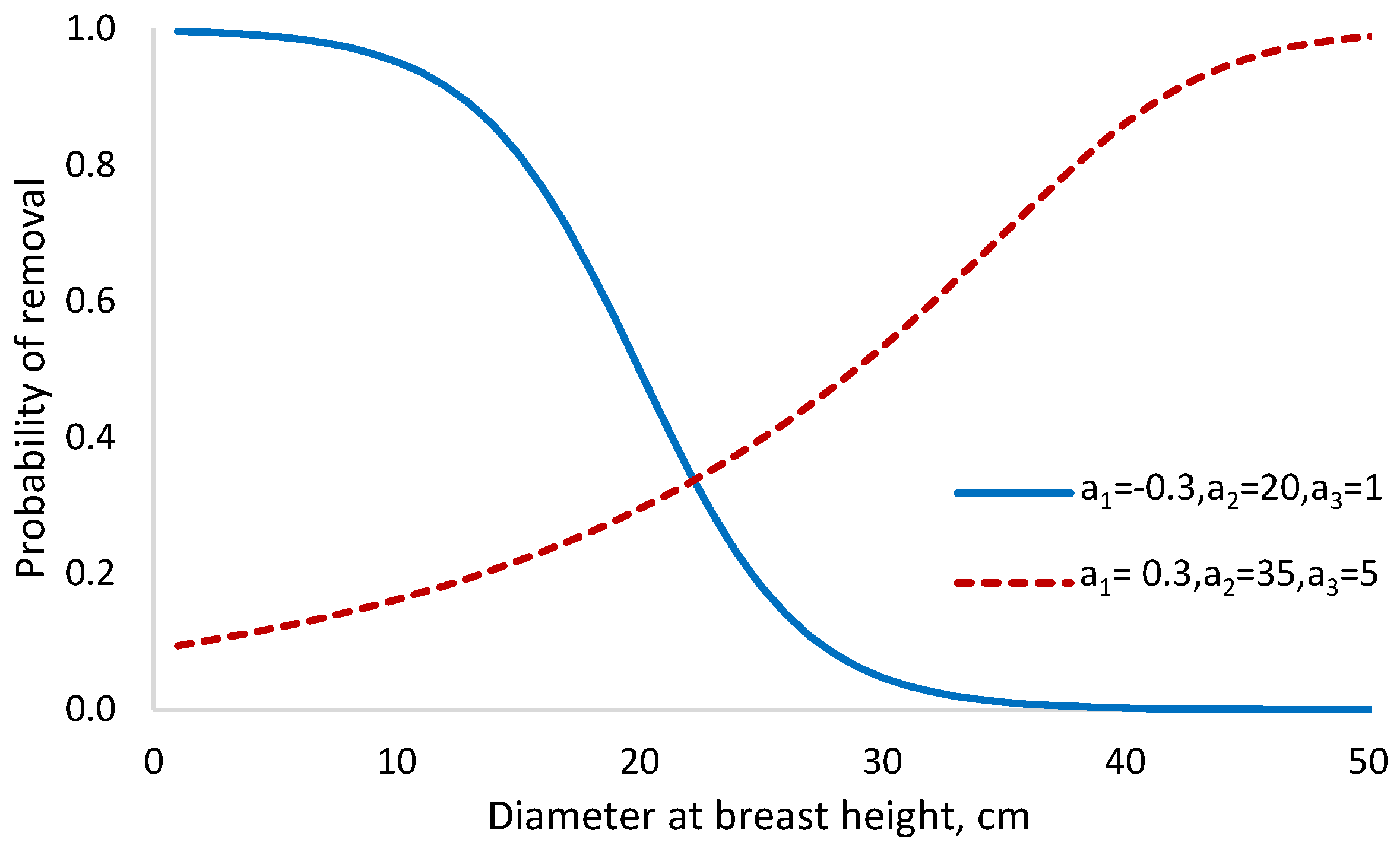
The method developed in this study optimized the cutting schedule of an even-aged pre-commercial Korean pine stand. When the optimization algorithm evaluated a certain cutting schedule, stand development was simulated until the clear-felling year. Cuttings were simulated according to the management schedule. Four decision variables were optimized for each partial cutting: the number of years to the cutting event, and three parameters of a thinning intensity curve (Figure 1). For clear-felling, only the number of years since the last partial cutting was optimized.
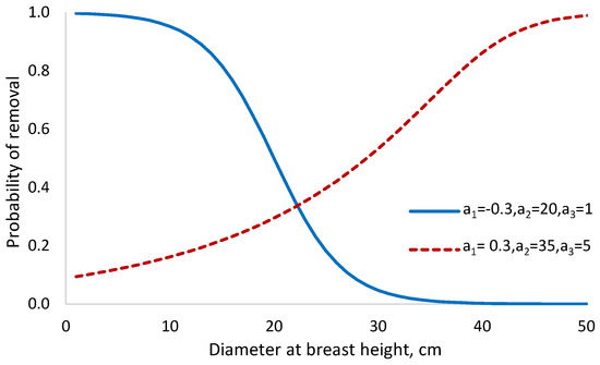
Figure 1.
Examples of thinning intensity curves. In the deterministic simulation, the curve shows the proportion of trees removed from a certain diameter class. In stochastic simulation, the curve shows the probability that the tree is removed. The solid line represents thinning from below and the dashed line represents thinning from above.
The thinning intensity curve was defined by the following formula [30]:
where is the thinning intensity (proportion of removed trees, or probability of removal) for diameter , and , , and are parameters optimized separately for each thinning treatment.
The stand was represented by a rectangular plot in which the diameters of all trees were known. Stand age and dominant height were used to calculate the site index of the stand (Equation (A1)). Site index was used as a predictor in diameter increment, survival, tree height, and cone yield models (Appendix A).
The stand establishment costs consisted of site preparation and planting work costs, the price of planted seedlings, and tending costs during the first years after planting. Altogether, the stand establishment costs were assumed to be CNY 17,400 per hectare. The cost estimates were based on discussions with several forester managers working in the Korean pine forests of the Heilongjiang province.
The development of the initial stand was simulated in one-year steps using the diameter increment and survival models described in Appendix A. Survival was simulated by multiplying the frequency of the tree (number of trees per hectare represented by one tree of the plot) by the survival probability.
The thinning treatment was simulated by using the thinning intensity curve (Equation (1)). The proportion of the tree’s frequency indicated by the thinning intensity curve was harvested. For example, in a 0.01-ha plot, each tree represents 100 trees per hectare. If the thinning intensity of a tree was 0.3, thirty trees per hectare were harvested, and 70 trees were left to continue growing. The heights of the harvested trees were calculated with a height model (Equations (A3) and (A4)), after which a taper model (Equation (A10)) was used to calculate the volumes of harvested timber assortments. Assortment volumes were multiplied by their stumpage prices to obtain the net income of the harvests.
Cone yield was calculated every year, and all cones were harvested. The cone yield model is a tree-level model that predicts the number of cones as a function of trunk diameter (diameter at breast height, dbh), stand basal area (G), basal area of larger trees (BAL), and site index (SI) (Equations (A5)–(A7)). The model is a zero-inflated negative binomial model. It consists of two sub-models, one for the number of cones and another for the probability that the tree has no cones. The number of cones in a tree is obtained as follows:
where is the probability of “extra zeroes” (probability that the tree does not produce cones) and Count is the number of cones in case the tree is producing cones [7,31,32]. The predictors of the cone count model are dbh, BAL, G, and SI, and the predictors of the extra zero model are dbh and BAL. If the tree is small and faces much competition (has high BAL) the likelihood that it is not producing cones is high.
The cone harvesting cost () was calculated using the following equation:
where is the fixed cost of harvesting cones from a stand (transporting the team and equipment to the stand, etc.), is the fixed harvesting cost per tree (emplacing ladders, climbing the tree, etc.), is the number of trees per hectare, is the cost of collecting one cone (dropping the cone from the tree, collecting it from the ground, etc.), and is the number of harvested cones per hectare.
All parameters of the cost functions were obtained by interviewing several foresters working in various forest farms in the Heilongjiang province. Based on the interviews, the following values were used: CNY 200 (per ha), CNY 4 (per tree), and CNY 2 (per cone). The cone harvesting team usually climbs only a part of the trees. While in the tree, they drop cones also from adjacent trees using a long stick. The parameter represents the average climbing cost per tree. The average length of harvested cones is typically around 14 cm, and their diameter is around 8 cm. There are usually more than 100 seeds in a cone [33]. The price of cones, when sold from a forest farm, was also obtained by interviewing foresters. The price used in this study was CNY 7 (per cone).
2.2. Stochastic Simulation
In stochastic optimization, every cutting schedule that was inspected during the optimization run was simulated 100 times by adding stochastic elements to the simulation. The stochastic parts were the diameter increment of trees, cone yield, tree survival, and tree selection in a thinning treatment.
To simulate annual variation in diameter increment, an autoregressive model (AR) was fitted using tree ring data collected from 40 to 50-year-old Korean pine stands, located in the Mengjiagang forest farm (Heilongjiang province). A total of 140 annual growth ring cores from 98 trees were available for fitting the model. The following model was obtained:
where is the growth index in year t and is the standard deviation of the residual (0.1308).
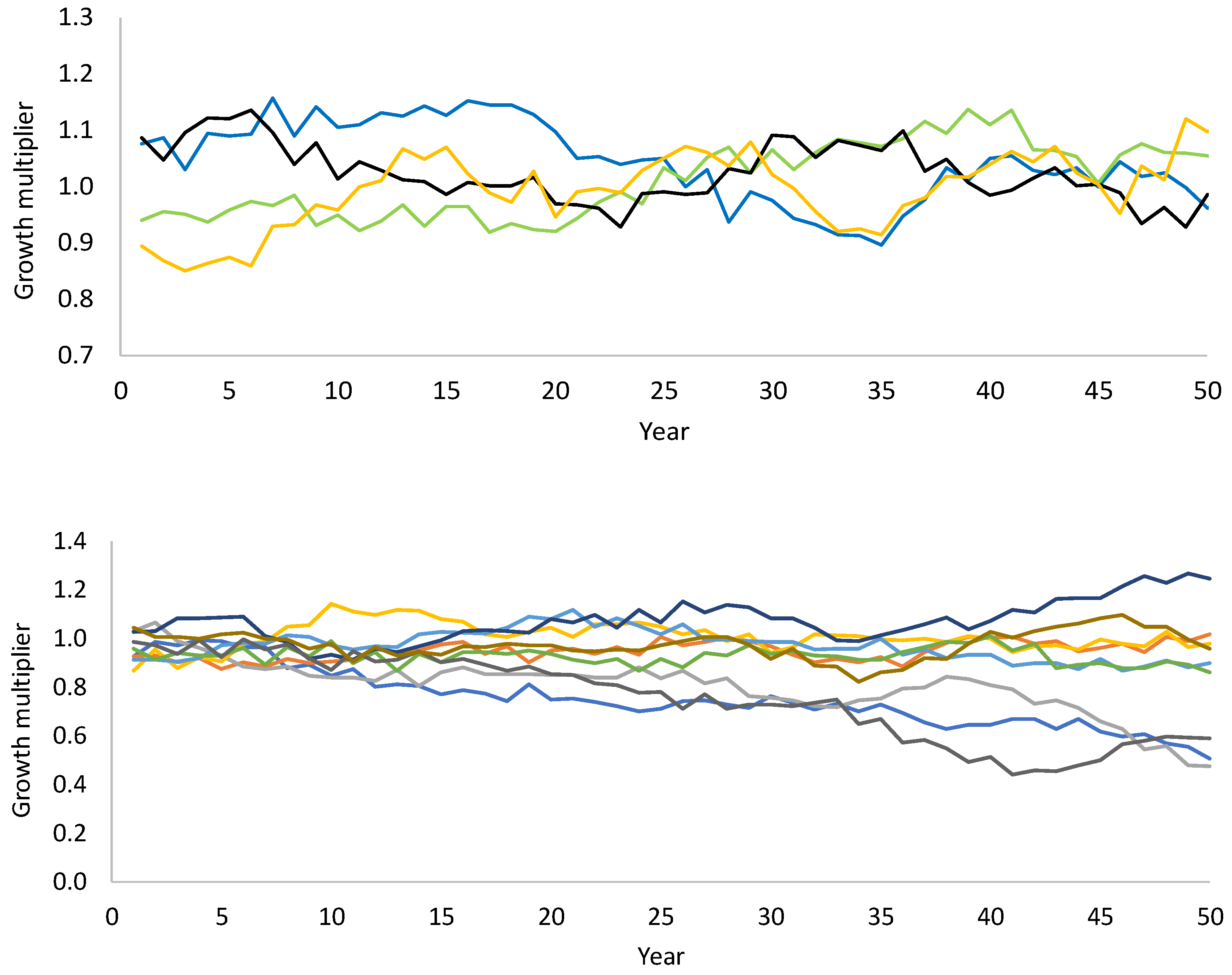
The model was used to generate 200-year stochastic growth scenarios. A random number corresponding to the residual variance was drawn from the normal distribution N [0, 0.1308] and added to the prediction. The 200-year sequences were converted into growth multipliers by dividing all values of the sequence by the average value of the 200-year scenario (Figure 2). In stochastic simulation, the predicted annual diameter increments of trees were multiplied by the value of the stochastic growth scenario in the same year. The time series produced in this way are stationary because the mean, variance, and autocorrelation structure do not change over time [34].
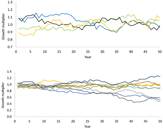
Figure 2.
Examples of stochastic growth scenarios. Different colors indicate different realizations of the same stochastic model. (Top): stationary scenarios without trend; (bottom): non-stationary scenarios with stochastic linear trends.
Due for instance to climate change, the level of tree growth may change in the future, even substantially. The growth may improve at northern latitudes because temperatures are rising, and precipitation may also increase in the north [35]. On the other hand, the climate may become more irregular and include severe drought periods, which may decrease tree growth [21]. Therefore, optimizations were also conducted under the assumption that future tree growth may change in a trend-like manner. Non-stationary growth scenarios were produced for these optimizations as follows:
where is the growth multiplier for year t, is a normally distributed random number with a mean equal to zero and a standard deviation equal to 0.01 (N [0,0.01]) and is the growth multiplier for year t obtained from Equation (4). The random number () was constant for different years of a certain scenario but different for different scenarios. Figure 2 (bottom) shows examples of growth scenarios that include trends.
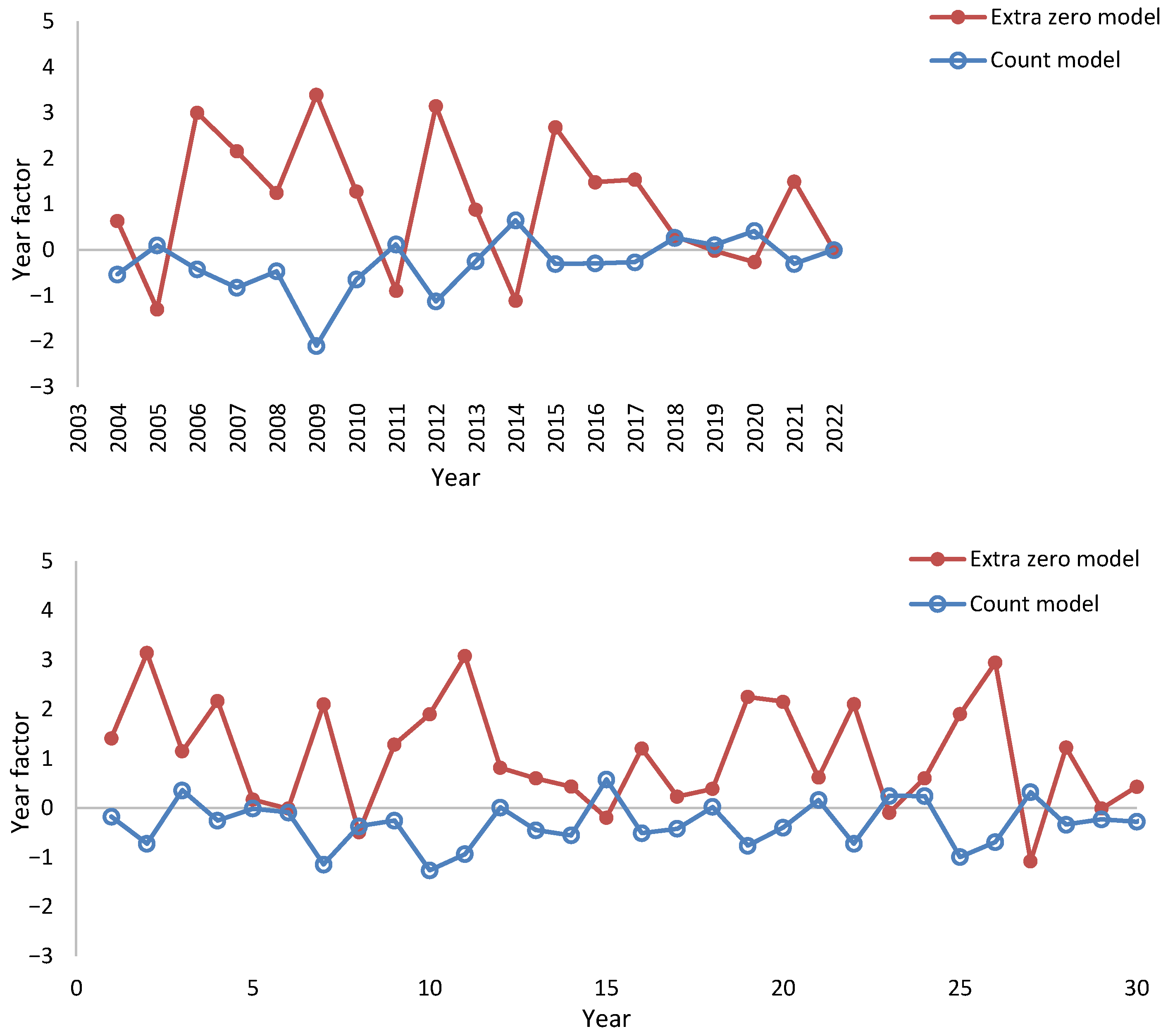
The cone yield models (Equations (A5) and (A6)) had year factors both in the count model and the extra zero model (Figure 3 top). In Korean pine, every third year is typically a “mast year” with high cone and seed production. This periodicity can be seen in Figure 3 (top) where years 2005, 2008, 2011, 2014, and 2020 could be taken to represent mast years. This periodicity is not perfect. For example, 2017 was not better than 2016 or 2017. Mast years have a high year factor for the count model and a low year factor for the model of extra zeroes.

Figure 3.
Modeled year factors of the count and extra zero models ((top), see Equations (A5) and (A6)). The (lower) diagram shows a stochastic 30-year scenario for the year factors of the cone yield model.
The year factors of the fitted cone yield model were used to produce stochastic cone yield scenarios. First, the mean year factor of the count model and its standard deviation were calculated separately for the mast years (mean 0.0915, standard deviation 0.413) and other years (mean −0.495, standard deviation 0.611). These statistics were used to create stochastic scenarios assuming that the year factors are normally distributed and there is no other temporal correlation than the three-year periodicity. The number of years to the first mast year was randomized (0, 1, or 2 were randomly selected).
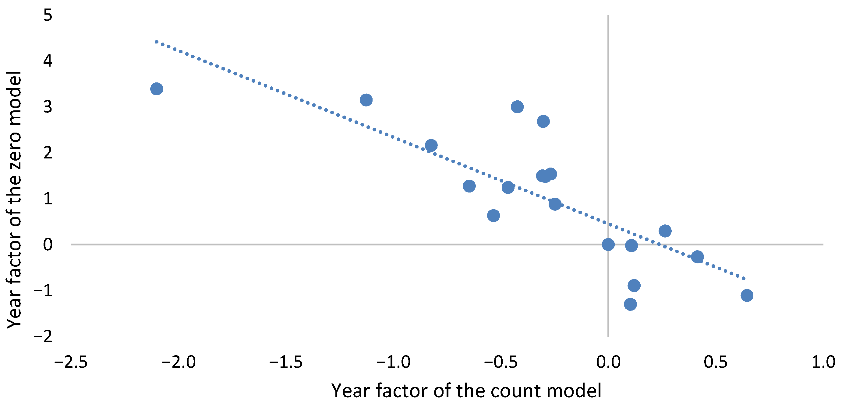
Figure 3 (top) shows that the year factors of the count and extra zero models are negatively correlated, which means that when the cone count is high, there are only a few trees that have no cones and vice versa. This correlation was used to fit a linear regression model where the year factor of the extra zero model was predicted from the year factor of the count model (Figure 4).
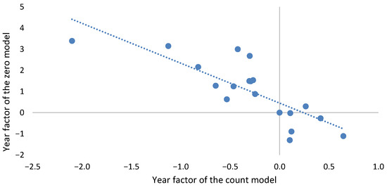
Figure 4.
Correlation between the year factors of the cone count and extra zero models (Equations (A5) and (A6)) and a regression line fitted to the year factor data.
The mean and standard deviation of the residuals of this model were 0.00001 and 0.8514, respectively. The scenarios of the year factors of the extra zero model were produced by calculating a prediction from Equation (6), using the stochastic year factor of the count model as the predictor. Then, a normally distributed random number corresponding to the residual of Equation (6) was added to the prediction. Figure 3 (bottom) shows that this method produces temporal series that have the same features as the modeled year factors.
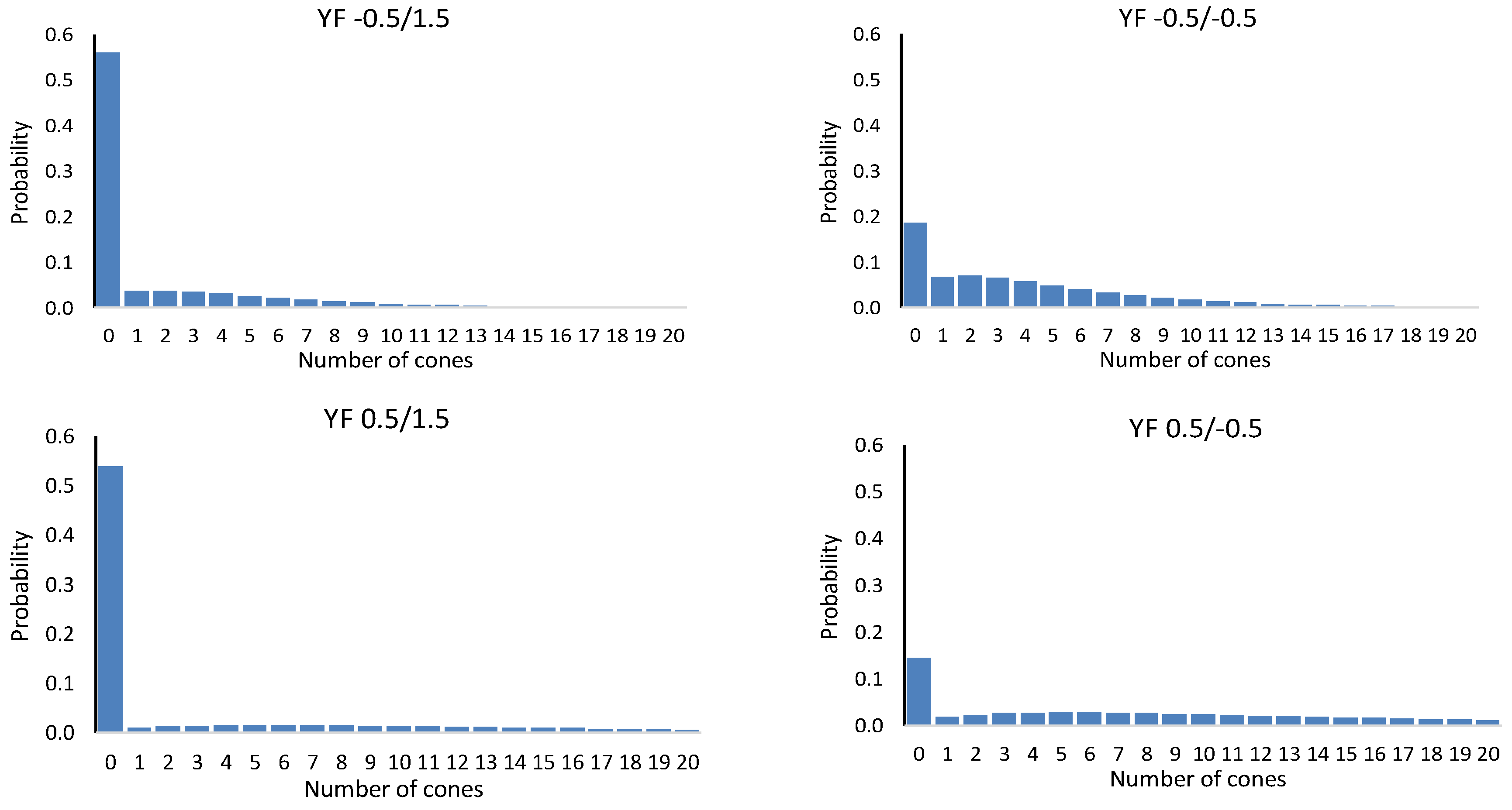
In deterministic simulation, all trees with the same diameter had the same number of cones in a certain year and stand (Equation (2)). In the stochastic simulation, the distribution of the cone count was calculated for every tree (see [7] for details). The number of cones was drawn randomly from the probability distribution [7]. Figure 5 shows four examples of the distribution for the same tree with four different combinations of the year factors of the count and extra zero models.
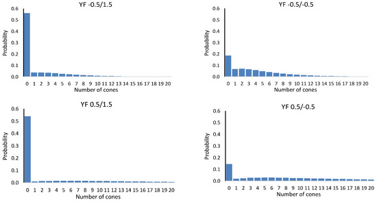
Figure 5.
Probability distribution of the number of cones when the tree diameter is 25 cm, stand basal area is 20 m2ha−1, basal area in larger trees (BAL) is 10 m2ha−1, and site index is 15 m, for different values of random year factors. In the abbreviation YF xx/yy, xx is the year factor of the cone count model and yy is the year factor of the model for extra zeros. The average year factors in the modeling data were −0.31 for the count model and 1.04 for the model for extra zeros.
In stochastic simulation, tree survival and removal were also stochastic. To simulate survival, the one-year survival probability, obtained from the model (Equation (A9)) was compared with a uniform random number U [0,1]. The tree survived if the random number was smaller than the survival probability. When simulating thinning treatments, the thinning intensity obtained from Equation (1) was compared to a uniformly distributed random number (U [0,1]). The tree was removed if the random number calculated for the tree was smaller than the thinning intensity.
2.3. Optimization
The differential evolution (DE) algorithm [36,37] was used to find the optimal combination of cutting intervals and optimal parameters of the thinning intensity curves. The objective variable was net present value (NPV), evaluated from the year of stand establishment to infinity. The simulation calculated the NPV of the first rotation (NPVRotation) as follows:
where is the revenue (income) and is the cost in year t, T is the rotation length and r is the discount rate in percent (3% used in this study). The stand establishment costs at the beginning of the rotation were common for timber and cone production. In later years, revenues and costs were calculated separately for timber and cone production. Cone revenue was equal to cone price multiplied by the number of cones. The cone harvesting cost was calculated with Equation (2). Net revenues from timber sales were calculated using stumpage prices. A stumpage price is the difference between roadside price and harvesting cost. The stumpage prices were 900, 825, 750 and 350 CNY/m3 for large sawlogs, medium-sized sawlogs, small sawlogs, and poles, respectively. NPV to infinity (NPV) was calculated by assuming that the same rotation is repeated to infinity.
DE is a population-based method. It operates with several solution vectors, which are combined according to the procedures of the algorithm [36,37]. The solution vectors are modified for several rounds (iterations). The optimal solution is the best solution vector at the end of the last iteration. A detailed explanation of using DE in the optimization of forest management is provided by Pukkala [38]. The study also shows that DE outperforms several other optimization methods in forestry-related optimization problems.
In the current study, the number of solution vectors was 90 (ten times the number of optimized variables). The number of iterations was 50. Since the optimization algorithm has stochastic elements, all optimizations were repeated 10 times, and the best result was reported.
First, net present value (NPV), calculated with a three percent discount rate was maximized, using deterministic simulation. Stand development was simulated until clear-felling. To calculate NPV to infinity, it was assumed that the same rotation would be repeated indefinitely.
Second, stochastic optimization was conducted by maximizing the average NPV of 100 stochastic outcomes, using stationary growth scenarios. In these optimizations, diameter increment, cone yield, tree survival, and tree removal in thinning treatments were simulated stochastically as explained above.
Third, the stochastic optimizations were repeated using the non-stationary scenarios for the tree growth multiplier. These optimizations were conducted for risk-neutral decision-makers as well as for risk-avoiders and risk-seekers. The risk-neutral decision-maker maximized the mean NPV of the 100 stochastic outcomes of the management schedule. The risk avoider maximized the 10% percentile of the distribution of NPV, and the risk seeker maximized the 90% percentile [12]. For the risk avoider, the purpose was to find a management schedule for which the worst outcomes are good [11]. The risk seeker wanted to find a management outcome that is good under favorable states of nature, although the likelihood of such a favorable situation may be low [11].
For fair comparisons of deterministic and stochastic solutions, the management schedule obtained from deterministic optimization was simulated under the same 100 growth and cone yield scenarios that were used in stochastic optimization.
3. Results
3.1. Stationary Growth Scenarios
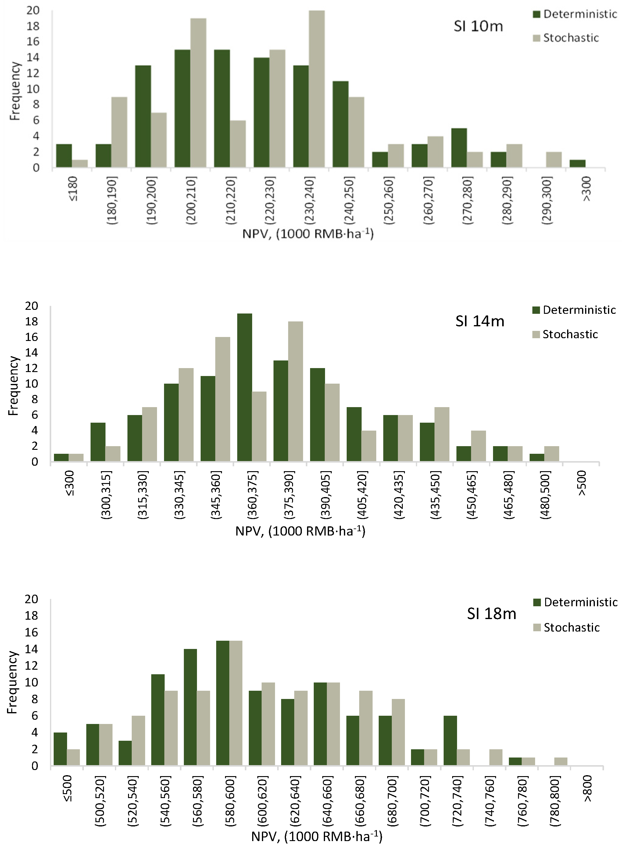
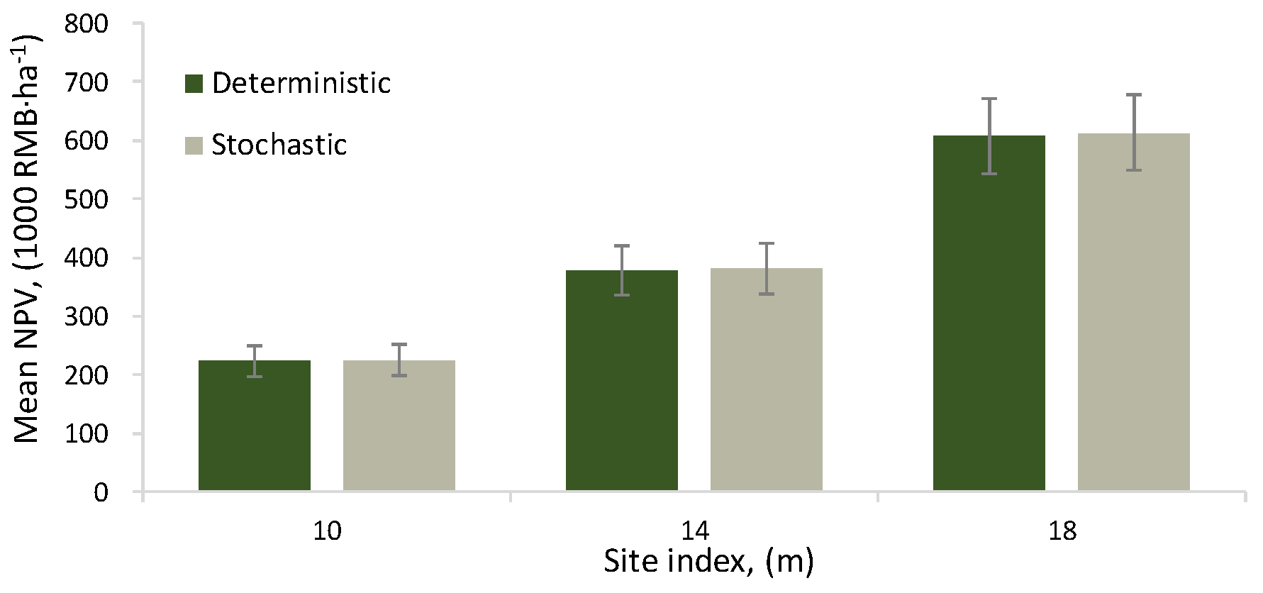
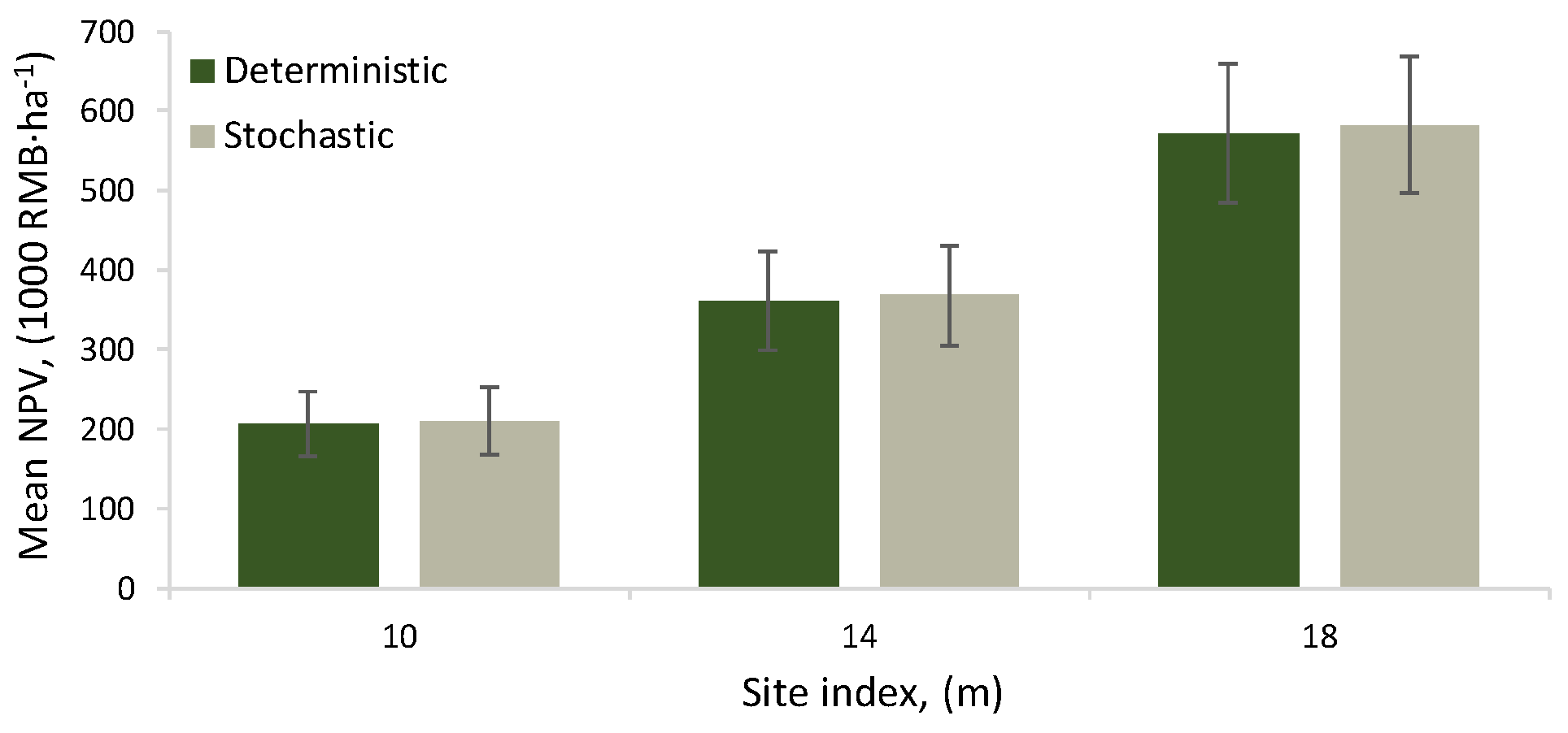
When the stochastic growth scenarios were stationary, the distributions of the NPVs calculated for the optimal management schedule indicate slight superiority of the stochastic optima; under the same set of growth and cone yield scenarios, the stochastic optima produced fewer poor outcomes (low NPVs) and a higher number of good outcomes (Figure 6). However, the superiority of the stochastic optima in the mean NPV of the 100 outcomes (Figure 7) was small, 0.4% in site index 10 m, and 0.9% in site indices 14 and 18 m.
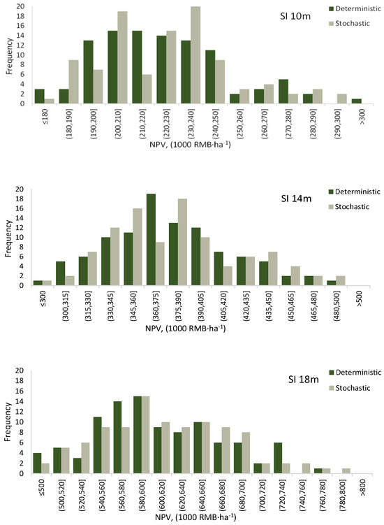
Figure 6.
Distribution of net present value when the optimal management scenarios, based on either deterministic or stochastic optimization, were simulated stochastically under 100 different scenarios for tree growth and cone yield.
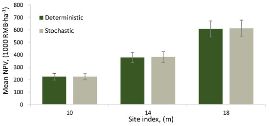
Figure 7.
The mean net present value when the management schedule based on deterministic or stochastic optimization was simulated stochastically under 100 different scenarios for tree growth and cone yield. The vertical line shows the standard deviation of the net present value.
All thinnings were to be conducted from above in both deterministic and stochastic optima (Table 1). The first thinning was prescribed a few years later in the stochastic optima, but otherwise, there were no systematic differences between the deterministic and stochastic optima (Table 1). Logically, optimal rotation lengths were shorter for better sites.

Table 1.
Cutting years and types of thinning in the deterministic and stochastic optima for different site indices and risk attitudes. In stochastic optimization, the stochastic growth scenarios are either stationary (no trend) or non-stationary (the growth scenarios include stochastic trends).
3.2. Non-Stationary Growth Scenarios
When stochastic optimization was conducted under non-stationary scenarios for tree growth, the differences between the mean NPV were clearer in favor of stochastic optimization, 1.8% in site indices 10 and 18 m, and 1.7% in site index 14 m. In these comparisons, both deterministic and stochastic optima were simulated under the same 100 scenarios, which were non-stationary for tree growth, and stationary for cone yield.
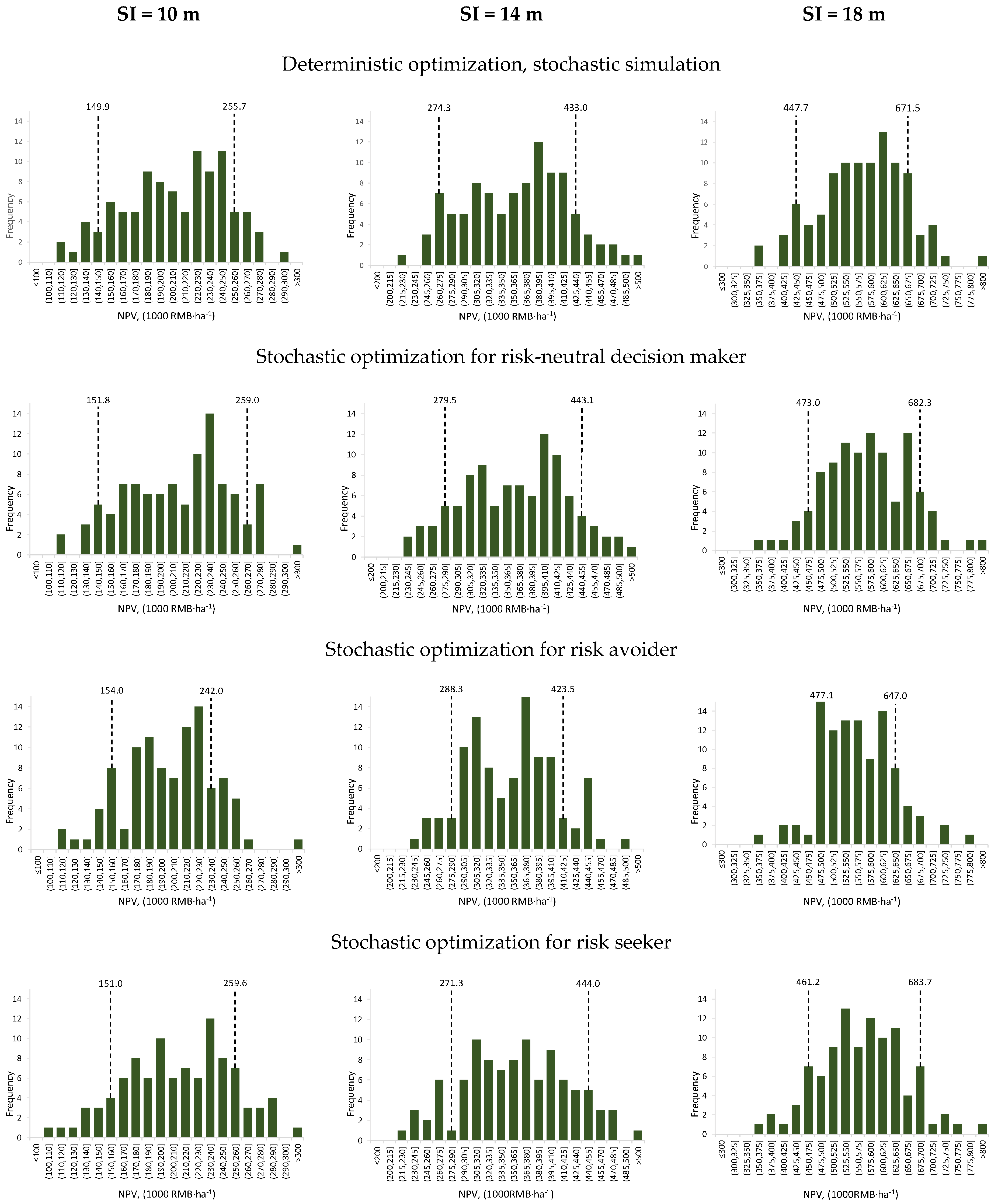
The stochastic optimizations were also conducted for risk-averse and risk-seeking decision-makers, by maximizing the 10% or 90% percentile of the distribution of NPVs. Figure 8 shows that the results were logical. The management schedules that were optimal for the risk avoider had fewer bad outcomes (low NPVs) compared to the schedules that were optimal for a risk-neutral decision-maker. Figure 8 also shows that the 10% percentiles were higher in the NPV distributions for the management schedules that were optimal for the risk avoider.
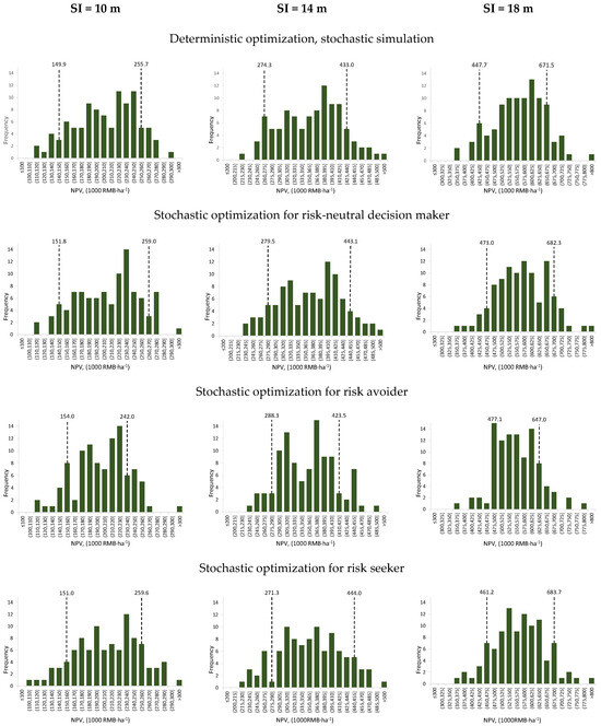
Figure 8.
Distribution of net present value when the optimal management schedule for risk-neutral, risk-averse, or risk-seeking decision-makers is simulated stochastically, under 100 scenarios for tree growth and cone yields, and the growth scenarios are non-stationary. The dashed vertical lines show the 10% and 90% percentiles of the distribution of net present value.
When management was optimized for a risk seeker, the NPV distributions of the optimal management schedules included a higher number of good outcomes (high NPV), compared to the schedules that were optimal for risk-neutral and risk-averse decision-makers (Figure 8). The 90% percentile of the NPV distribution was highest for the schedules that were optimal for the risk seeker. However, Figure 8 shows that the differences in the NPV distributions were small. The mean NPVs of the 100 scenarios were also close to each other in deterministic and stochastic optima, or for different risk attitudes (Figure 9).
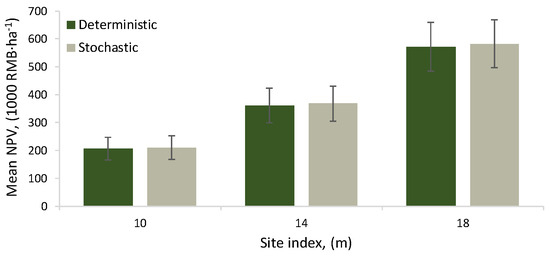
Figure 9.
The mean net present value in 100 stochastic simulations of the optimal management schedule based on deterministic or stochastic optimization. The stochastic optima are for risk-neutral decision-makers. The results are based on 100 stochastic simulations of the optimal management schedule under 100 non-stationary growth scenarios and 100 stationary cone yield scenarios.
Comparisons of the management schedules based on deterministic and stochastic optimizations revealed some systematic differences (Table 1). First, the optimal rotation lengths for risk-neutral decision-makers were shorter under non-stationary growth scenarios, as compared to stationary scenarios. The difference ranged from 5 to 14 years. Second, the optimal rotation length of the risk seeker was always shorter than for the other risk attitudes, the difference to the risk-neutral being 5 to 25 years in cases where the growth scenarios were non-stationary. Third, none of the optimal management schedules for risk avoiders had any removal in the first thinning, which means that the optimal management schedules for risk avoiders included only one thinning treatment. Despite these systematic differences in optimal management, the profitability of management (distribution of NPV) was almost equal in all cases.
3.3. Yield Estimates, Degree of Uncertainty
The results indicate that the optimized management is rather similar in stochastic and deterministic optimization, suggesting that it is not necessary to include stochasticity in management planning. However, stochastic simulations provide information on the possible range of variation in incomes, timber, and cone yields. In addition, the expected yield (mean) may be different in deterministic and stochastic calculations.
In the case of Korean pine, which produces timber and edible seeds, the calculations indicate that the predicted timber yield was almost the same in deterministic and stochastic simulations (Table 2). However, the cone yield estimates were much higher when they were based on repeated stochastic simulations. The likely reason for this is that the cone yields obtained from a certain stand are not normally distributed, and the exceptionally good cone yields increase the average outcome of the stochastic simulations.

Table 2.
Yield estimates for the optimal management schedules based on deterministic optimization, obtained from a single deterministic simulation or 100 simulations under stationary stochastic growth and cone yield scenarios.
Stochastic calculations also provide information on the precision of the yield estimates. Table 3 shows that, under the assumption of stochastic but stationary tree growth and cone yield, the coefficient of variation in wood production estimates was very small, only 1.3 to 1.6%. The relative coefficient of variation was much higher for cone yield, ranging from 9.0 to 11.0%. The coefficient of variation of the net present value was close to that of the cone yield because most of the NPV is accounted for by cone sales. However, when the stochastic growth scenarios were assumed to be non-stationary, the uncertainty of wood production estimates increased greatly, which also increased the coefficient of variation of net present value.

Table 3.
Average yield and coefficient of variation in net present value (NPV), wood production (WP) and cone yields (CY) when the stochastic optimization was conducted using stationary or non-stationary scenarios for tree growth and stationary scenarios for cone yield.
4. Discussion
Previous studies have used stochastic optimization with the scenario technique to find the best management schedule for a tree stand [39]. In most previous studies, tree growth and timber prices have been stochastic. Our study is the first where the management of Korean pine plantations was optimized under stochastic cone production. In Korean pine, cones generate more income than timber sales [7]. Cone production is more erratic than tree growth, and it could therefore be hypothesized that considering this variation in management optimization could have a significant effect on the optimization results. However, our study does not support this hypothesis.
The results of our study revealed that the optimal management schedule of Korean pine plantations was similar in stochastic and deterministic optimization. The distributions of the net present values differed only a little when both management schedules were simulated stochastically, under the same 100 stochastic scenarios for tree growth and cone yield. Therefore, our results show that deterministic optimization is “sufficient” in Korean pine management if only optimal prescriptions are required and a single anticipatory optimum is targeted.
Stochastic optimization resulted in better management, although the difference to deterministic optimization was small. The benefit of using stochastic optimization increased when the amount of stochasticity increased. The same was observed in the study by Pukkala and Kellomäki [10] where stochastic optima were not much better under normal variation (based on historical data) in tree growth and timber price. However, the benefit increased when the variation among the stochastic growth and price scenarios increased. Our results suggest that a risk seeker cuts earlier than the other risk attitudes. In this respect, the results agree with those of Huang et al. [14] who found that a risk-averse landowner would likely cut later.
Even if the differences in the optimization results were small, stochastic analysis has other benefits as it provides more information for the decision-maker, as compared to deterministic analyses. Stochastic simulation makes it possible to assess the reliability of the yield estimates and generate confidence limits for the forecasts. In addition, stochastic optimization makes it possible to include the risk attitude of the decision-maker in the optimization.
An important finding was that the estimates of expected cone yields differed when they were based on deterministic or stochastic simulations, stochastic calculations resulting in higher average cone yield estimates. Therefore, there are several reasons to conduct stochastic analyses, even though their effect on management prescriptions may be small.
In the stochastic simulation, it is possible to realistically consider the effect of the size of the cone yield on the cone harvesting costs. In our calculations, the net income per kilogram of cones decreased with decreasing cone yield because cone collection involved fixed harvesting costs. The approach used in our study resembles the method of Tahvanainen et al. [29], who optimized the joint production of timber and marketed mushrooms in Picea abies stands in Finland. In their study, the mushroom harvesting costs consisted of the travel costs to the forest and mushroom picking costs in the forest. Since mushroom yields vary greatly from year to year, the net income per kilogram of mushrooms also varied between years. To calculate the expected net income from mushroom harvesting, Tahvanainen et al. [29] simulated 200 stochastic outcomes for the mushroom yield in a particular year. They assumed that mushrooms were not collected when the harvesting cost was higher than the selling price of the mushrooms.
One reason for the small difference between deterministic and stochastic optimization may be that stochastic optimization is more complicated. The effect of stochasticity on the thinning removal and mortality could be decreased by using larger plots in simulation and using more than 100 scenarios in simulation. However, these modifications would increase the time consumption of the optimization runs.
Abundant flowering and cone production consume photosynthesized carbon hydrates and may affect the growth of the trees [40]. This means that the time series of tree growth and cone yield are most probably cross-correlated. This correlation was ignored in the current study, due to the lack of suitable empirical data. This shortcoming could be mitigated in future studies, by collecting tree ring data from the same plots in which cone yields have been monitored. However, as cone yield depends on tree growth, the trends of the non-stationary growth scenarios create trends also in cone production.
On the other hand, our study showed that stationary annual variation in tree growth does not have much effect on optimal management or timber yield estimates. Correlating the stochastic annual variation in diameter increment with the annual variation in cone production would most probably not alter this conclusion.
The current study used both stationary and non-stationary scenarios for tree growth. The non-stationarity assumption may be more realistic because the level of tree growth may change gradually and in different directions. It is not fully understood how future climate will affect tree growth [15,22,23]. Positive effects have often been suggested for northern latitudes, based on the increasing temperature and non-decreasing precipitation. Bagaram and Tóth [15] assumed that the effect of climate change on diameter increment can be positive or negative, but the likelihood of positive effects is greater. Bagaram and Tóth [15] also assumed that the effect of climate change depends on the stage of stand development.
Some of the estimates of the effects of climate change may be positively biased because they ignore the adverse effect of the increased irregularity in the rain regime, for example [21]. In addition, climate change may lead to wind damage and increased incidences of pathogen and pest outbreaks, which all decrease tree growth.
Climate change may affect cone yields and tree growth differently. For example, drought periods may decrease tree growth and survival, but they may trigger abundant flowering and cone crops [41,42]. Our study ignored these relationships.
The methodology applied in the current study represents the anticipatory approach to stochastic optimization where management is not adjusted according to changes in the state of nature. Each optimization produced only one management prescription, which means that the stand is to be cut always in the same year, independently of the realized rate of tree growth, for example. Therefore, the trees are cut at smaller trunk diameters when tree growth is slow and larger diameters in case of favorable conditions for tree growth.
Since the financial maturity for cutting is closely related to tree diameter, the adaptive approach to management optimization may provide better guidelines for forest management than the anticipatory method used in our study [43,44]. Under long-term fluctuations or non-stationary trends in the growth rate of trees, it would be better to optimize the mean tree diameter that triggers a cutting event, instead of optimizing cutting years. Since the optimal diameter for cutting depends on the stand density, a function showing the cutting diameter as a function of the stand basal area could also be optimized.
A simple rule for adaptive cone harvesting would be to refrain from cone harvesting when the harvesting cost is greater than the selling price of the cones [29]. The same principle could also be used at the tree level: cones are not collected from those trees for which the harvesting cost would be higher than the selling price of the cones.
Temporal variation in timber price may have a stronger impact on optimal management than temporal variation in tree growth, especially when the growth scenarios are stationary. Due to the limited availability of statistical data on timber prices in China, constant prices were used in our study. The cone prices and the harvesting costs of cones were also constant. Cone prices most probably vary less than timber prices, which depend on economic fluctuations in the construction businesses. However, the harvesting cost per kilogram of cones is lower when the cone yield is abundant. This relationship was not explicitly considered in our optimizations. However, the selling price of cones may also be lower in good cone years, which means that the difference between the selling price and harvesting cost may remain rather constant.
In addition to providing information on the amount and significance of the annual variation in tree growth and cone production, the study also developed new models for the stand dynamics and cone production of Korean pine plantations. These models can be used in many ways in forest planning calculations for the most important tree species of the Heilongjiang province.
5. Conclusions
Stochastic optimization with the scenario method was employed to find the optimal management strategies for Korean pine plantations in the joint production of timber and cones. The results showed that the optimized stand management was similar in stochastic and deterministic analysis. However, stochastic simulation offers information on the reliability of the yield and income estimates. An important result of the analyses was that the predicted timber and cone yields differed in deterministic and stochastic calculations. In addition, stochastic optimization makes it possible to consider the risk attitude of the decision-maker in management optimization.
Author Contributions
Conceptualization, T.P. and X.J.; methodology, T.P.; software, T.P.; formal analysis Q.T., T.P. and X.J.; data curation, X.J., L.D. and F.L.; writing—original draft preparation, Q.T., T.P. and X.J.; writing—review and editing L.D. and F.L.; visualization, Q.T., T.P. and X.J.; supervision, X.J. and T.P.; project administration, X.J.; funding acquisition, L.D. and F.L. All authors have read and agreed to the published version of the manuscript.
Funding
This research was funded by the Natural Science Foundation of China (32071758 and U21A20244).
Data Availability Statement
The original contributions presented in the study are included in the article, further inquiries can be directed to the corresponding authors.
Acknowledgments
The authors would like to thank Xiaochun Wang, College of Forestry of Northeast Forestry University (NEFU), for providing the ring data support for this study.
Conflicts of Interest
The authors declare no conflicts of interest.
Appendix A. Models Used in the Study
- Site index model
Various algebraic difference models (ADA models) were tested as the site index model [45,46,47,48,49,50,51]. A total of 392 measurements from 75 plots were available for site index modeling. The Lundqvist and Korf model [46] was evaluated to be the best (R2 = 0.91, RMSE = 1.42 m and AIC = 1392):
where and are the dominant heights in two measurement occasions, and and are the ages at the times of the two measurements.
The site index was defined to be the dominant height at 40 years. The site index was calculated as follows:
where is the dominant height, and is the stand age.
- 2.
- Individual-tree height model
The number of tree height observations was 26,220, measured from 6673 trees in 137 permanent sample plots. Of the tested model types, the Näslund model [45,52,53] was used. Two different variants of the height model were fitted. The first one used dominant height as a predictor, and it is suitable for simulations where all thinnings are from below. The model is as follows (R2 = 0.91, RMSE = 1.07 m, and AIC = 80760):
where is the tree height (m), is the diameter (cm) of tree in plot , was the dominant height of plot , and , , are random factors. The other variant can be used in simulations where thinning from above is allowed (R2 = 0.86, RMSE = 1.34 m, and AIC = 91666):
where is the tree height (m), is the diameter (cm) of tree in plot , is the stand age of plot , and is the site index (m) of plot .
- 3.
- Cone yields model
The cone yield model is based on the zero-inflated negative binomial (ZINB) model, which consists of two parts: a count model predicts the non-zero using a negative binomial model, and a zero-inflation model predicts the probability of the tree not producing cones using a logistic model. The dataset included 16884 tree-level cone counts from 1760 individual trees. The data were collected in 24 permanent plots on 282 measurement occasions. The two sub-models of the ZINB model were as follows (AIC = 80,760):
The cone yield estimate for a tree is calculated as follows:
where is the diameter (cm) of the tree, is the basal area (m2·ha−1), is the basal area of the trees larger than the subject tree (m2·ha−1), and are indicator variables for different years.
- 4.
- Diameter increment and survival models
We used the optimization-based method [54] to prepare the data and optimize the parameters. The diameter increment model obtained from the optimization is as follows:
where is the annual diameter increment (cm). The survival model is:
where is the one-year survival rate.
- 5.
- Taper model
The taper model developed by Kozak in 2004 was used for estimating tree volume and calculating the volumes of different timber assortments. The model is as follows [8]:
where is the diameter outside bark (cm) at meters above the ground, is the diameter outside bark at the breast height, and is the total tree height. ; ; ; .
References
- Xu, Z.; Dai, H.; Li, X. Rational management of broadleaved/Pinus koraiensis (Korean pine) forest and improvement of woodland productivity in north-east China. Temp. For. Ecosyst. 1986, 59–67. [Google Scholar]
- Bao, L.; Kudureti, A.; Bai, W.; Chen, R.; Wang, T.; Wang, H.; Ge, J. Contributions of Multiple Refugia during the Last Glacial Period to Current Mainland Populations of Korean Pine (Pinus Koraiensis). Sci. Rep. 2015, 5, 18608. [Google Scholar] [CrossRef]
- Shalizi, M.; Khurram, S. Socio-economic importance of chilgoza pine forest of Afghanistan: A survey based assessment. Asian J. Sci. Technol. 2016, 7, 3556–3559. [Google Scholar]
- Yoshimoto, A.; Asante, P.; Konoshima, M. Stand-Level Forest Management Planning Approaches. Curr. For. Rep. 2016, 2, 163–176. [Google Scholar] [CrossRef]
- Kuuluvainen, T.; Tahvonen, O.; Aakala, T. Even-Aged and Uneven-Aged Forest Management in Boreal Fennoscandia: A Review. AMBIO 2012, 41, 720–737. [Google Scholar] [CrossRef] [PubMed]
- Huang, S. Duanzhi Caisongta—Causing the “Little Year” of Pinus koraiensis seeds. Wild Plant Res. 1985, 3, 23. [Google Scholar]
- Jin, X.; Li, F.; Pukkala, T.; Dong, L. Modelling the Cone Yields of Korean Pine. For. Ecol. Manag. 2020, 464, 118086. [Google Scholar] [CrossRef]
- Jin, X.; Pukkala, T.; Li, F.; Dong, L. Optimal Management of Korean Pine Plantations in Multifunctional Forestry. J. For. Res. 2017, 28, 1027–1037. [Google Scholar] [CrossRef]
- Pasalodos-Tato, M.; Pukkala, T.; Calama, R.; Cañellas, I.; Sánchez-González, M. Optimal Management of Pinus Pinea Stands When Cone and Timber Production Are Considered. Eur. J. For. Res. 2016, 135, 607–619. [Google Scholar] [CrossRef]
- Pukkala, T.; Kellomaki, S. Anticipatory vs Adaptive Optimization of Stand Management When Tree Growth and Timber Prices Are Stochastic. Forestry 2012, 85, 463–472. [Google Scholar] [CrossRef]
- Kangas, J. Incorporating Risk Attitude into Comparison of Reforestation Alternatives. Scand. J. For. Res. 1994, 9, 297–304. [Google Scholar] [CrossRef]
- Pukkala, T.; Kangas, J. A Method for Integrating Risk and Attitude Toward Risk into Forest Planning. For. Sci. 1996, 42, 198–205. [Google Scholar] [CrossRef]
- Moss, I.; Robinson, A. A Simple Way to Incorporate Uncertainty and Risk into Forest Harvest Scheduling. For. Ecol. Manag. 2015, 359, 11–18. [Google Scholar] [CrossRef]
- Huang, Y.-K.; Bawa, R.; Dwivedi, P.; Zhao, D. Stochastic Dynamic Optimization for Forest Rotation with Uncertain Stumpage Prices. For. Sci. 2022, 68, 389–398. [Google Scholar] [CrossRef]
- Bagaram, M.B.; Tóth, S.F. Multistage Sample Average Approximation for Harvest Scheduling under Climate Uncertainty. Forests 2020, 11, 1230. [Google Scholar] [CrossRef]
- Pukkala, T. Optimizing Continuous Cover Management of Boreal Forest When Timber Prices and Tree Growth Are Stochastic. For. Ecosyst. 2015, 2, 6. [Google Scholar] [CrossRef]
- Pukkala, T. Multiple Risks in Multi-Objective Forest Planning: Integration and Importance. For. Ecol. Manag. 1998, 111, 265–284. [Google Scholar] [CrossRef]
- Susaeta, A.; Gong, P. Optimal Harvest Strategy for Even-aged Stands with Price Uncertainty and Risk of Natural Disturbances. Nat. Resour. Model. 2019, 32, e12211. [Google Scholar] [CrossRef]
- Brazee, R.; Mendelsohn, R. Timber Harvesting with Fluctuating Prices. For. Sci. 1988, 34, 359–372. [Google Scholar] [CrossRef]
- Albert, M.; Hansen, J.; Nagel, J.; Schmidt, M.; Spellmann, H. Assessing Risks and Uncertainties in Forest Dynamics under Different Management Scenarios and Climate Change. For. Ecosyst. 2015, 2, 14. [Google Scholar] [CrossRef]
- Elli, E.F.; Sentelhas, P.C.; Bender, F.D. Impacts and Uncertainties of Climate Change Projections on Eucalyptus Plantations Productivity across Brazil. For. Ecol. Manag. 2020, 474, 118365. [Google Scholar] [CrossRef]
- Garcia-Gonzalo, J.; Borges, J.G.; Palma, J.H.N.; Zubizarreta-Gerendiain, A. A Decision Support System for Management Planning of Eucalyptus Plantations Facing Climate Change. Ann. For. Sci. 2014, 71, 187–199. [Google Scholar] [CrossRef]
- Garcia-Gonzalo, J.; Pais, C.; Bachmatiuk, J.; Weintraub, A. Accounting for Climate Change in a Forest Planning Stochastic Optimization Model. Can. J. For. Res. 2016, 46, 1111–1121. [Google Scholar] [CrossRef]
- Buongiorno, J.; Zhou, M. Adaptive Economic and Ecological Forest Management under Risk. For. Ecosyst. 2015, 2, 4. [Google Scholar] [CrossRef]
- Lauer, C.J.; Montgomery, C.A.; Dietterich, T.G. Spatial Interactions and Optimal Forest Management on a Fire-Threatened Landscape. For. Policy Econ. 2017, 83, 107–120. [Google Scholar] [CrossRef]
- Bushaj, S.; Büyüktahtakın, İ.E.; Haight, R.G. Risk-Averse Multi-Stage Stochastic Optimization for Surveillance and Operations Planning of a Forest Insect Infestation. Eur. J. Oper. Res. 2022, 299, 1094–1110. [Google Scholar] [CrossRef]
- Pasalodos-Tato, M.; Pukkala, T.; Alboreca, A.R. Optimal Management of Pinus Pinaster in Galicia (Spain) under Risk of Fire. Int. J. Wildland Fire 2010, 19, 937–948. [Google Scholar] [CrossRef]
- Bright, G.; Price, C. Valuing Forest Land under Hazards to Crop Survival. Forestry 2000, 73, 361–370. [Google Scholar] [CrossRef]
- Tahvanainen, V.; Miina, J.; Pukkala, T.; Kurttila, M. Optimizing the Joint Production of Timber and Marketed Mushrooms in Picea Abies Stands in Eastern Finland. J. For. Econ. 2018, 32, 34–41. [Google Scholar] [CrossRef]
- Sun, Y.; Jin, X.; Pukkala, T.; Li, F. A Comparison of Four Methods for Automatic Delineation of Tree Stands from Grids of LiDAR Metrics. Remote Sens. 2022, 14, 6192. [Google Scholar] [CrossRef]
- Xiao, Y.; Zhang, X.; Ji, P. Modeling Forest Fire Occurrences Using Count-Data Mixed Models in Qiannan Autonomous Prefecture of Guizhou Province in China. PLoS ONE 2015, 10, e0120621. [Google Scholar] [CrossRef]
- Tang, W.; He, H.; Tu, X.M. Applied Categorical and Count Data Analysis; CRC Press: Boca Raton, FL, USA, 2023; ISBN 978-1-00-086397-0. [Google Scholar]
- Zhang, M.-Y.; Su, C.-X.; Lu, C.-H. Cones Structure and Seed Traits of Four Species of Large-Seeded Pines: Adaptation to Animal-Mediated Dispersal. Ecol. Evol. 2020, 10, 5293–5301. [Google Scholar] [CrossRef]
- Box, G.E.P.; Jenkins, G.M.; Reinsel, G.C.; Ljung, G.M. Time Series Analysis: Forecasting and Control; John Wiley & Sons: Hoboken, NJ, USA, 2015; ISBN 978-1-118-67492-5. [Google Scholar]
- Kellomäki, S.; Peltola, H.; Nuutinen, T.; Korhonen, K.T.; Strandman, H. Sensitivity of Managed Boreal Forests in Finland to Climate Change, with Implications for Adaptive Management. Philos. Trans. R. Soc. B-Biol. Sci. 2007, 363, 2339–2349. [Google Scholar] [CrossRef]
- Storn, R.; Price, K. Differential Evolution—A Simple and Efficient Heuristic for Global Optimization over Continuous Spaces. J. Glob. Optim. 1997, 11, 341–359. [Google Scholar] [CrossRef]
- Díaz-Yáñez, O.; Arias-Rodil, M.; Mola-Yudego, B.; Olabarria, J.; Pukkala, T. Simulating the Effects of Wind and Snow Damage on the Optimal Management of Norwegian Spruce Forests. Forestry 2019, 92, 406–416. [Google Scholar] [CrossRef]
- Pukkala, T. Population-Based Methods in the Optimization of Stand Management. Silva Fenn. 2009, 43, 211. [Google Scholar] [CrossRef]
- Valsta, L.T. A Scenario Approach to Stochastic Anticipatory Optimization in Stand Management. For. Sci. 1992, 38, 430–447. [Google Scholar] [CrossRef]
- Obeso, J.R. The Costs of Reproduction in Plants. New Phytol. 2002, 155, 321–348. [Google Scholar] [CrossRef]
- Maguire, W.P. Are Ponderosa Pine Cone Crops Predictable? J. For. 1956, 54, 778–779. [Google Scholar]
- Matthews, J.D. Factors Affecting the Production of Seed by Forest Trees. For. Abstr. 1963, 24, 1–13. [Google Scholar]
- Gong, P. Adaptive Optimization for Forest-Level Timber Harvest Decision Analysis. J. Environ. Manag. 1994, 40, 65–90. [Google Scholar] [CrossRef]
- Gong, P. Risk Preferences and Adaptive Harvest Policies for Even-Aged Stand Management. For. Sci. 1998, 44, 496–506. [Google Scholar] [CrossRef]
- Peschel, W. Mathematical methods for deriving growth laws for trees and stands with application experiences. Tharandter Forstl. Jahrburch 1938, 89, 169–247. (In German) [Google Scholar]
- Korf, V. A mathematical definition of standing volume growth law. Lesn. Pr. 1939, 18, 337–339. [Google Scholar]
- Schumacher, F.X. A new growth curve and its application to timber yield studies. Forestry 1939, 37, 819–820. [Google Scholar]
- Richards, F.J. A Flexible Growth Function for Empirical Use. J. Exp. Bot. 1959, 10, 290–301. [Google Scholar] [CrossRef]
- Sloboda, B. Describing the growth process with first-order differential models. Mitt. Bad.Württemb. Forstl. Vers. Forsch. Anst. 1971, 32. (In German) [Google Scholar]
- McDill, M.E.; Amateis, R.L. Measuring Forest Site Quality Using the Parameters of a Dimensionally Compatible Height Growth Function. For. Sci. 1992, 38, 409–429. [Google Scholar] [CrossRef]
- Cao, Y.; Sun, Y. Generalized algebraic difference site index model for Chinese fir plantation. J. Nanjing For. Univ. 2017, 60, 79. [Google Scholar]
- Näslund, M. Forest research intitute’s thinning experiments in Scots pine forests. Medd. Stat. Skogsförsöksanst. 1937, 29, 169. (In Swedish) [Google Scholar]
- Mehtätalo, L.; de-Miguel, S.; Gregoire, T.G. Modeling Height-Diameter Curves for Prediction. Can. J. For. Res. 2015, 45, 826–837. [Google Scholar] [CrossRef]
- Dong, L.; Pukkala, T.; Li, F.; Jin, X. Developing Distance-Dependent Growth Models from Irregularly Measured Sample Plot Data—A Case for Larix Olgensis in Northeast China. For. Ecol. Manage. 2021, 486, 118965. [Google Scholar] [CrossRef]
Disclaimer/Publisher’s Note: The statements, opinions and data contained in all publications are solely those of the individual author(s) and contributor(s) and not of MDPI and/or the editor(s). MDPI and/or the editor(s) disclaim responsibility for any injury to people or property resulting from any ideas, methods, instructions or products referred to in the content. |
© 2024 by the authors. Licensee MDPI, Basel, Switzerland. This article is an open access article distributed under the terms and conditions of the Creative Commons Attribution (CC BY) license (https://creativecommons.org/licenses/by/4.0/).

