Article

Prediction of the Global Distribution of Arhopalus rusticus under Future Climate Change Scenarios of the CMIP6

1
Key Laboratory of Beijing for the Control of Forest Pests, College of Forestry, Beijing Forestry University, Beijing 100083, China
2
College of Forestry, Shenyang Agricultural University, Shenyang 110866, China
*
Author to whom correspondence should be addressed.
Forests 2024, 15(6), 955; https://doi.org/10.3390/f15060955
Submission received: 15 April 2024 / Revised: 18 May 2024 / Accepted: 25 May 2024 / Published: 30 May 2024
(This article belongs to the Section Forest Health)

Abstract

:
Arhopalus rusticus is a significant forestry pest known for its destructive impact on various host plants. This species, commonly found in coniferous forests across the Northern Hemisphere, has successfully spread to regions like New Zealand, Australia, and South America. This research is based on the known distribution sites of A. rusticus. Projections are made for the potential global distribution of A. rusticus under historical climatic conditions (1970–2000) and future climatic conditions (2081–2100) for the four forcing scenarios of the Coupled Model International Comparison Program 6 (CMIP6). The aim was to analyze the effects of climate change on the distribution range of this pest and its invasion trend in the southern hemisphere, and to support relevant departments in enhancing the effectiveness of forestry pest control strategies. The study utilized the Biomod2 software package in R to compare six models: generalized linear models (GLMs), generalized additive models (GAMs), multivariate adaptive regression splines (MARSs), artificial neural networks (ANNs), classification and regression trees (CTAs), and random forests (RFs) for modeling species distributions. The optimal model was selected based on evaluation indexes such as AUC and TSS. Projections of A. rusticus distribution under historical and future climate scenarios were created. The prediction results were visualized using ArcGIS software (version 10.2) to classify fitness levels and calculate distribution areas. Based on evaluation metrics, random forests (RFs) demonstrated the highest average assessment index scores, indicating high prediction accuracy (AUC = 0.99, TSS = 0.91, Kappa = 0.93). Model predictions revealed that, under historical climatic conditions, A. rusticus was predominantly found in northern Europe, eastern Asia, eastern and southwestern coastal regions of North America, and there were also highly suitable regions in parts of the southern hemisphere, including central and southwestern Argentina, southern Australia, New Zealand, and South Africa. Among these models, each of the CMIP6’s different climate prediction scenarios had a significant impact on the predicted distribution of A. rusticus. The SSP126 scenario depicted the broadest range of suitability, while the SSP585 scenario presented the narrowest and, overall, the extent of highly suitable regions was contracting. Multi-model predictions suggested that the potential distribution area of A. rusticus during the period of 2081–2100 would likely expand compared to that of 1970–2000, ranging from an increase of 1.13% (SSP126) up to 6.61% (SSP585), positively correlating with the level of radiative forcing. Notably, the most substantial growth was observed in potentially low-suitability region, escalating from 1.17% (SSP126) to 5.55% (SSP585). The distribution of A. rusticus shows decreasing trends from coastal areas to inland areas and from high to low level suitability of regions, and further expansion into the southern hemisphere under future climate conditions. Therefore, quarantine efforts at ports of entry should be strengthened in areas that are not currently infested but are at risk of invasion, and precise preventive measures should be strengthened in areas that are at risk of further expansion under future climatic conditions to prevent its spread to inland areas.

1. Introduction

Arhopalus rusticus (Linnaeus, 1758) (Coleoptera: Cerambycidae) is a destructive pest that targets pine, fir, cypress, and other coniferous trees by drilling into them. This insect is particularly harmful to weakened coniferous trees, displaying a high level of selectivity towards its host trees [1]. A. rusticus typically goes through one generation every 2 to 3 years. Larvae overwinter in the host xylem, emerging in late March and producing fine powder as a sign of infestation. By late April, mature larvae create pupal chambers in the sapwood to pupate. In mid to late June, adult beetles reach their peak population, mating and laying eggs without needing to replenish nutrients. The eggs are laid under the tree bark, with an incubation period of 2–3 weeks. The first hatched larvae feed under the bark before moving inward to feed on the xylem, ultimately causing damage to the trees [2].
A. rusticus is primarily found in coniferous forests in Siberia, Sweden, Norway, Inner Mongolia, Tajikistan, China, Korea, and Japan. Its distribution is more prevalent in coastal areas compared to inland regions. As the latitude increases, the emergence of adult beetles is delayed and their activity period shortens [1]. Due to global trade, A. rusticus has successfully invaded New Zealand, Australia, and South America in the last century [3]. In the early 21st century, this species invaded Argentina and spread throughout the pine-producing regions of the province of Córdoba [4].
Global warming can impact the population dynamics of forestry pests, leading to changes in distribution areas and the colonization of new habitats [5]. It is difficult to predict their occurrence on a large scale using practical research methods such as statistical observation. Therefore, modeling the species distribution of forestry pests to predict their potential distribution under global warming scenarios can be more efficient than observing their movements [6]. It is important to clarify the changes in A. rusticus’s global range of suitable regions under future climate scenarios, which can be used to grasp its dispersal pattern and improve the control efficiency.
Species distribution models (SDMs) are numerical prediction tools that combine species occurrence or abundance results with environmental estimates, providing a better understanding of how climate limits the survival of organisms [7]. SDMs are diverse, and selecting modeling tools that can accurately predict species invasion risk requires a systematic and scientific approach [8]. Species-based distribution models have successfully predicted the potential distribution of several insects in China, including Monochamus alternatus [9], Anoplophora chinensis [10], and Anoplophora glabripennis [11]. The increase in temperature has led to the early emergence of some pests in spring and delayed overwintering in autumn, resulting in the early emergence of adults, prolongation of the occurrence period, and an increase in population sizes [12]. When environmental humidity is too high or too low, it leads to limited development or even a drastic reduction in the number of insects; the interaction of multiple climatic factors can have different effects on the survival and reproduction of forestry pests [13]. Therefore, environmental variables that contribute more to species survival and development should be selected before modeling to increase modeling accuracy. Biomod2, developed based on R, can perform a large number of operations using different kinds of models and comprehensively analyze the similarities and differences in all the results and uncertainties. Through the AUC value under the ROC curve [14], the true skill statistic (TSS) [15], and the Kappa score [16] model evaluation metrics, the model performance can be evaluated and validated. The optimal modeling to establish a prediction of the distribution of the species can then be filtered out. Currently, studies on A. rusticus have mainly focused on its biological characteristics [17,18], hazardous status [1], and control measures [19,20,21], but no further research has been carried out on the prediction of the potential distribution of A. rusticus. In a study on the development rate of the nymphal stage of A. rusticus and temperature, it was concluded that the development rate of A. rusticus accelerated with an increase in temperature [22]. Therefore, the correlation between distribution data and climate data was utilized to compare multiple models under future climate scenarios, and the optimal model was selected with the help of model evaluation indexes to establish a prediction of the potential distribution of A. rusticus globally which showed the highest predictive performance. This can guide the quarantine personnel at ports to implement the relevant quarantine measures to prevent the entry of A. rusticus according to the real-life situation, and provides a theoretical basis for the effective prevention and control of A. rusticus.

2. Materials and Methods

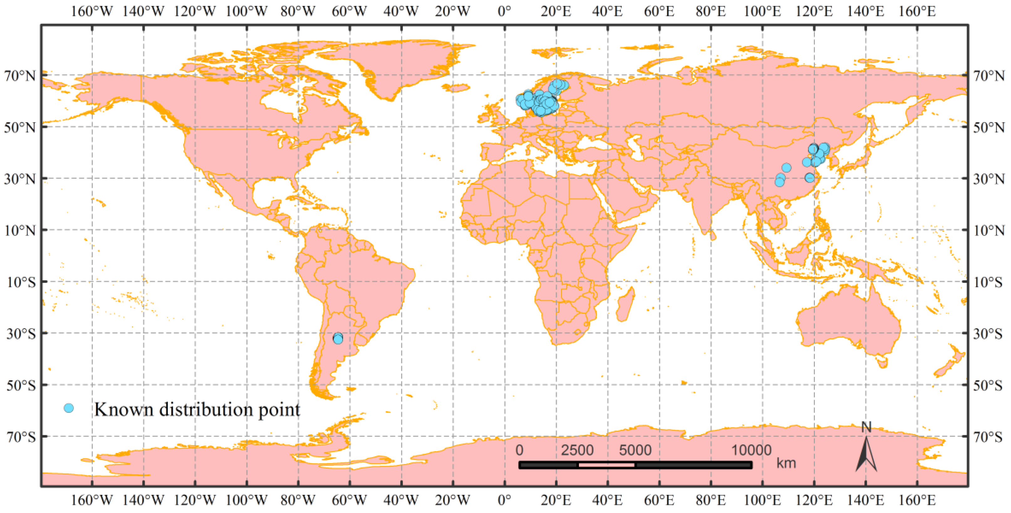
2.1. Occurrence Data Collection

The global geographic distribution data of A. rusticus are mainly collected from the global biodiversity information facility (GBIF, https://www.gbif.org (accessed on 21 December 2023)), and the geographic distribution coordinates are collected from the related literature. The distribution data of Sweden, Norway and China were selected as the native distribution points, and the distribution data of Argentina were selected as the invasive distribution points. The “CoordinateCleaner” package (https://ropensci.github.io/CoordinateCleaner/ (accessed on 21 December 2023)) in R was used to remove geographic distribution points with missing latitude and longitude, duplicated records, records falling into non-terrestrial areas, and those with high uncertainty. Then the “spThin” package (https://github.com/mlammens/spThin (accessed on 25 December 2023)) in R was used to sparse the data to retain only one distribution point in each 5 km × 5 km grid and to reduce the bias of the model prediction results caused by centralized sampling or data redundancy and, ultimately, retained a total of 305 distribution points for use in the modeling (Figure 1).

2.2. Acquisition and Selection of Bioclimate Variables

Global bioclimatic variables for the historical and future climatic conditions required for this study were downloaded from the WorldClim database (https://worldclim.org/ (accessed on 29 December 2023)), version 2.1, at a spatial resolution of 2.5 arc minutes for 19 bioclimatic variables. The data included the historical climate data from 1971 to 2000. The future climate data were selected from the medium-resolution model of the Beijing Climate Center Climate System Model (The Beijing Climate Center Climate System Model 2, BCC-CSM2-MR), which was obtained from the Sixth International Coupled Model Intercomparison Program (CMIP6) according to the actual situation of the current country (region) and the future development plan. Under four socio-economic development scenarios, SSP126, SSP245, SSP370, and SSP585, by the year 2100, radiative forcing stabilizes at approximately 2.6 watts per square meter (W/m2), 4.5 W/m2, 7.0 W/m2, and 8.5 W/m2, respectively, and climate data for the period from 2081 to 2100 are provided. Local bioclimatic data were extracted from 305 distribution records. Because the climate variables are prone to autocorrelation multicollinearity and data redundancy [23], which lead to biased prediction results, the 19 sampled bioclimatic variables need to be screened to exclude those with high correlation coefficients and low contribution rates. Principal component analysis (PCA) in the ranking technique was first used to reduce the dimensionality of the environmental variables, and the bioclimatic variables with loading coefficients greater than 0.3 in the first four principal components with cumulative contribution rates greater than 90% were retained. The remaining 14 climatic variables were subjected to Pearson correlation analysis, while the MaxEnt (version 3.4.4, https://biodiversityinformatics.amnh.org/open_source/maxent/ (accessed on 5 January 2024)) software was used for the initial modeling, and the variables with smaller contribution rates when the absolute value of the correlation coefficient was >0.80 were excluded according to the knife-cut method (Figure 2). Finally, these variables were screened to obtain the annual mean temperature (Bio1), mean diurnal range (Bio2), isothermality (Bio3), max. temperature of warmest month (Bio5), temperature annual range (Bio7), precipitation seasonality (Bio15), precipitation of the driest quarter (Bio17), and precipitation of the warmest quarter (Bio18), which were the key environmental variables influencing the distribution of A. rusticus.

2.3. Model Calculation and Evaluation

The presence–absence approach is theoretically closer to the real distribution of the species [24]; therefore, before modeling, 1000 pseudo-absences were produced prior to modeling using the R software’s Terra package and the “random” method at every point in the study area, excluding the presence points. The R (version 4.2.3) software’s “biomod2” package (https://biomodhub.github.io/biomod2/ (accessed on 15 February 2024)) implemented six algorithms: the generalized linear model (GLM) [25], generalized additive model (GAM) [26], multivariate adaptive regression spline (MARS) [27], artificial neural network (ANN) [28], classification tree model (CTA) [29], and random forest (RF) [30] to predict the potential distribution of A. rusticus. and evaluate the uncertainty caused by various SDMs. In order to ensure the independence of the training set and the dataset and to reduce the data having a spatial autocorrelation structure, k-fold in biomod2 was used to realize the cross-validation of the model [31]. An 80% subset was selected as the SDM training set and the remaining 20% of the dataset was used as the test set to evaluate the models’ performance. The relevant code can be found in the Supplementary Materials.
The models’ performances were assessed by the AUC value under the subject’s job characteristics (ROC) curve. TSS and Kappa were used to assess the model goodness-of-fit and validate the model prediction accuracy. Training and test datasets were used to distinguish observed events from background data and to calculate AUC values. AUC is independent of dataset size, but is limited by the scope of the study, which increases when the scope of the study is extended beyond the current range [32]. Kappa is influenced by the broadness of the species’ distribution, responds to changes in prevalence in a single-peak fashion, and was used to assess consistency [15]. TSS, which is not affected by prevalence, represents the sum of sensitivity (proportion of observed presences correctly predicted) and specificity (proportion of observed absences correctly predicted), and is used to determine model performance by checking classification accuracy after selecting a threshold [33].

2.4. Model Prediction and Visual Analytics

The biomod2 program was used to estimate the scores of AUC, Kappa, and TSS for the six models. AUC values ranged from 0 to 1, with model performance categorized as poor (0.6–0.7), fair (0.7–0.8), good (0.8–0.9), or excellent (0.91–1) [34]. The TSS values ranged from −1 to + 1, with low values indicating poorer prediction accuracy than random classification and high values indicating perfect agreement between observation and prediction [33]. The Kappa statistic ranges from −1 to +1, where +1 indicates consistent predictions and zero to lower values indicate performance that is not better than random. The high and low values of each assessment index scores for the various models were compared and the best model was selected. The prediction accuracies among models were compared so that the optimal model could be selected. Predictions were made for the potential distribution of A. rusticus under historical and future different climatic conditions using this optimal model saved in the default pathway, and the projected results were stored to the default pathway from the R software.
The predicted results (TIF format) were converted to raster format by using the Arc Toolbox toolkit in ArcGIS, the fitness probability layer was divided into fitness zones by combining with reclassification in the spatial analysis tool, and the fitness of A. rusticus was divided into four classes by using the natural intermittent point grading method, i.e., nonfamiliar zones, ≤0.06, low. The natural interspersed point classification method was used to categorize the fitness of A. rusticus into four classes: unsuitable region, ≤0.06; low-suitability region, 0.06~0.20; moderate-suitability region, 0.20~0.40; and high-suitability region, ≥0.40, and to assess its global distribution under the historical and future climate conditions. The reclassified raster layer was used to view the number of pixels in each suitability class, and the ratio of the number of pixels in each suitability class to the total number of pixels was calculated to derive the percentage of area in each suitability class.

3. Results

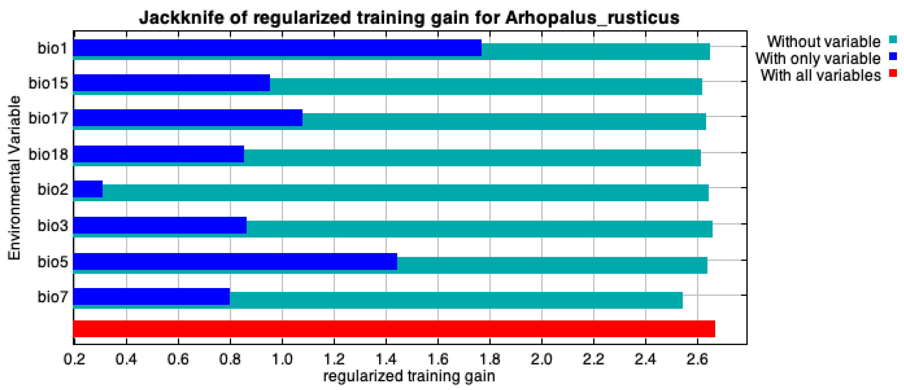
3.1. Comparison of the Contribution of Key Environmental Variables to Influencing the Distribution of A. rusticus

The geographic latitude and longitude information of 305 presence sites of A. rusticus and the screened eight environmental variables were imported into the MaxEnt model for Jackknife analysis (Figure 2). Among the eight environmental variables, Bio1 (annual mean temperature), Bio7 (temperature annual range), Bio18 (precipitation of the warmest quarter) and Bio17 (precipitation of the driest quarter) had the most significant contribution rates of 26.4%, 21.7%, 18.3% and 17.5%, respectively. If the probability of survival is greater than 0.5 as a measure of the optimum conditions, the conditions for the survival of A. rusticus are as follows: the average annual temperature is between 5 and 8 °C, the annual difference in temperature is between 23 and 29, the precipitation in the warmest season is between 100 and 250 mm, and the precipitation in the driest season is between 90 and 190 mm (Table 1).

3.2. Comparison of the Accuracy of the Prediction Results of Different Models

Comparing the evaluation metrics of the six models in Biomod2 (Figure 3), RF has the best simulation results, with AUC, TSS and Kappa reaching 0.99, 0.91, and 0.93, respectively. This was followed by GLM, MARS, and CTA, with model evaluation metrics that can reach AUC > 0.9, TSS > 0.9, and Kappa > 0.8. GAM has a relatively worse performance, with an AUC of 0.94, TSS of 0.76, and Kappa of 0.74. GAM had an AUC of 0.94, TSS of 0.76, and Kappa of 0.74. ANN had the worst simulation, with an AUC of 0.85, TSS of 0.67 and Kappa of 0.68. Therefore, the RF model was selected for the prediction of the potential distribution area of A. rusticus.

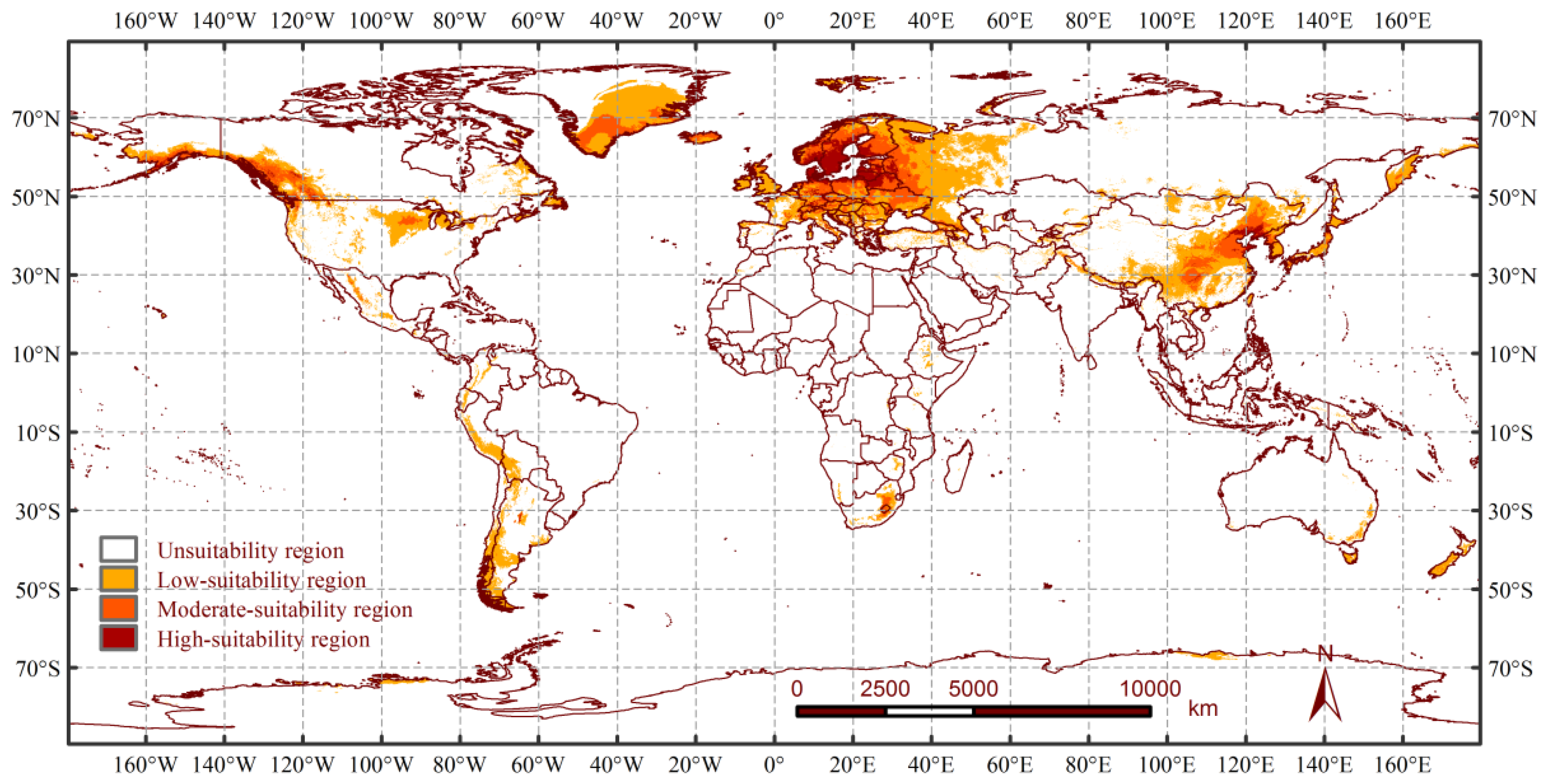
3.3. Potential Distribution Changes of A. rusticus under Historical Climatic Conditions

Under the historical climatic conditions, the RF model predicted that A. rusticus has a wide range of regions around the world, which can be distributed from 80° N to 80° S. The four levels of region were classified as unsuitable regions, low-suitability regions, moderate-suitability regions, and high-suitability regions, which were distinguished by four different colors from light to dark. As can be seen in the figure, the habitat of A. rusticus is mostly expanded gradually from the high-suitability region in the coastal area to the low-suitability region in the inland area. The coastal areas of the Gulf of Bothnia, the Baltic Sea, and Skagerrak Bay in Northern Europe, and the coastal areas of the Bohai Bay in Asia, and including Sweden, Finland, and Russia, are highly suitable regions for A. rusticus. Moderately suitable regions are mainly concentrated in the coastal areas of the United States and Canada in North America; Sweden, Finland, Iceland, Ukraine, Russia, and other countries in Northern Europe; Greenland in North America; China and Japan in Asia; and New Zealand in Oceania. The low-suitability regions are mainly distributed in the northeast and northwest of North America; most of the western part of northern Europe; the eastern part of Asia; and sporadically distributed in the southern hemisphere in the western coastal areas of South America, southern Africa, and the coastal areas of Australia (Figure 4). Globally, the ratio of low-, moderate-, and high-suitability regions to the global land area are 9.43%, 3.31%, and 0.87%, respectively (Table 2).

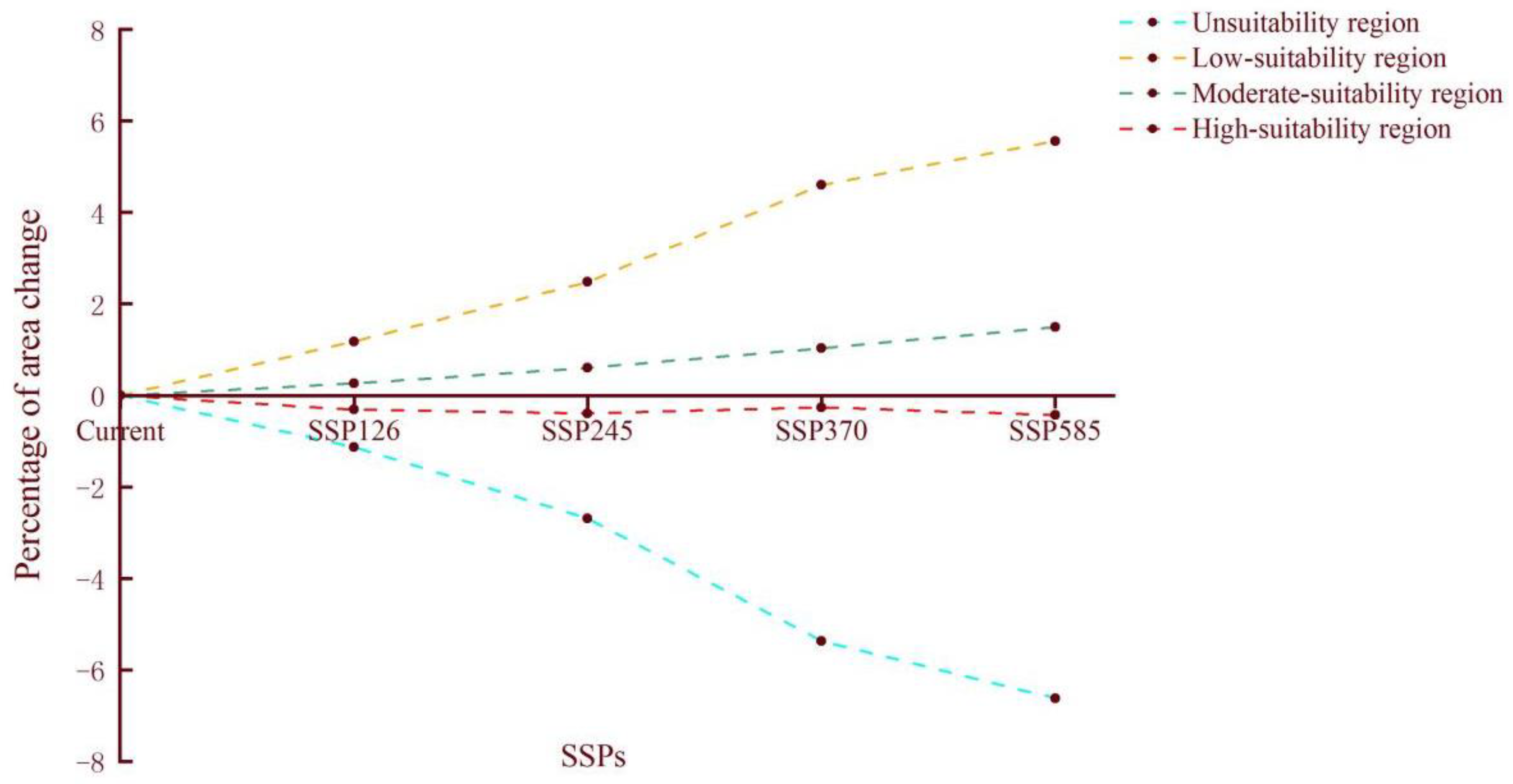
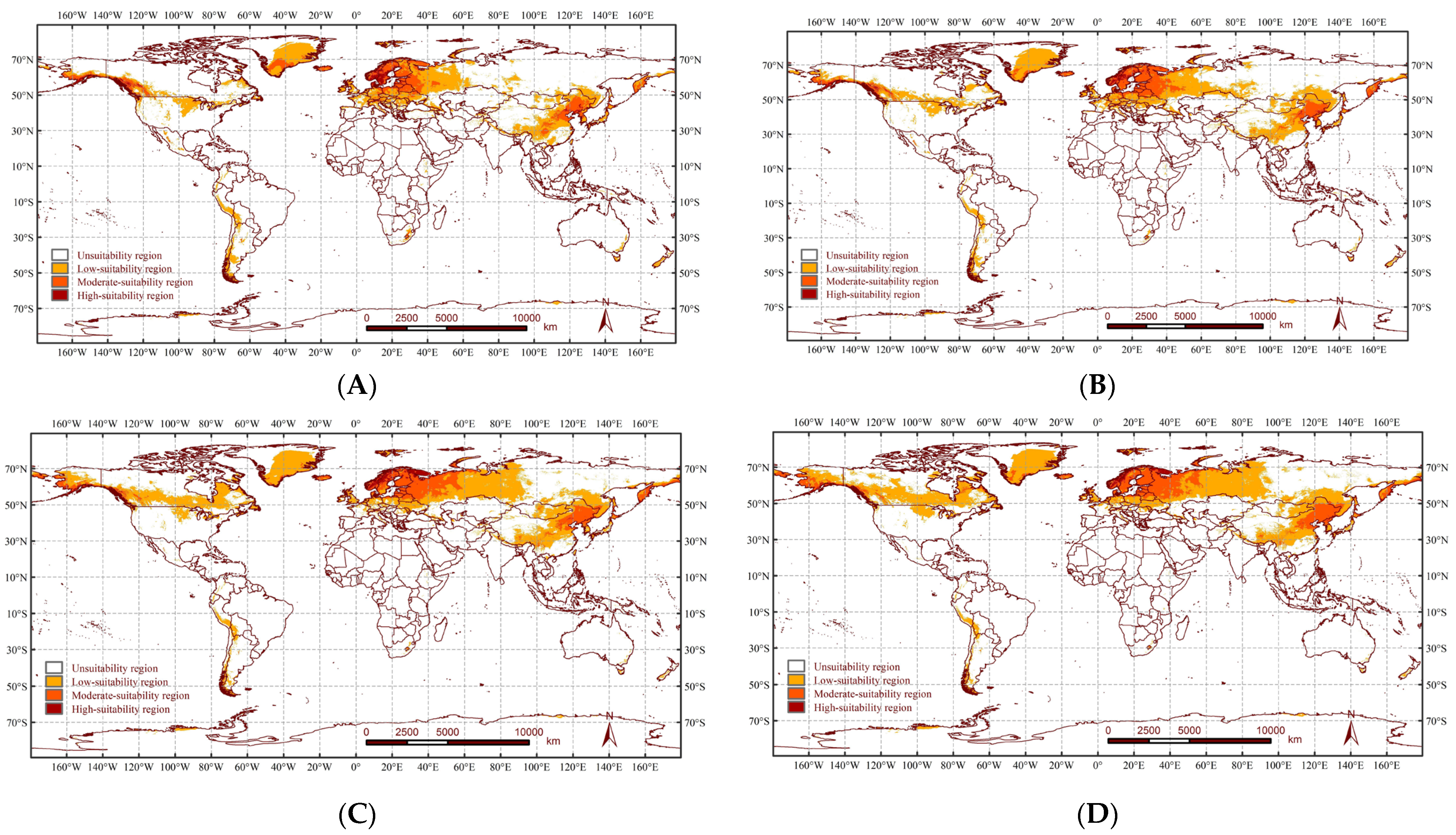
3.4. Comparison of the Potential Distribution of A. rusticus under Future Climate Scenarios

Using the current projections as a baseline, the percentage of the area of suitable regions, and the curve of change in the area of suitable regions in different years for each forcing scenario were plotted (Figure 5). Compared with the potential distribution under the historical climate, the global area of suitable regions under all forcing scenarios in the future (2081–2100) shows an increasing trend, and the proportion of the global land area increases with the increase in the radiative forcing level, which is 14.75% under SSP126, 16.29% under SSP245, 18.97% under SSP370, and 20.23% under SSP585, respectively.
The area of highly suitable regions showed different degrees of shrinkage, ranging from 0.26% to 0.43%; the areas of moderate- and low-suitability regions both showed a clear positive correlation with the radiative forcing level, with the increase in the area of moderately suitable regions ranging from 0.26% to 1.49%, and the increase in the area of low-suitability regions ranging from 1.17% to 5.54% (Table 2).
Projecting the global potential distribution of A. rusticus from 2081–2100 on a map under each scenario (Figure 6), disproportionate changes in the extent of each type of suitable region were observed under all forcing scenarios. The low- and medium-suitability zones in the western and southeastern regions of Russia and the low-suitability region in southern Canada showed increasing trends that were positively correlated with the degree of forcing; the potential distribution in the southern hemisphere did not change significantly, and although it did not show a significantly increasing trend, low-suitability zones still existed along the western coasts of South America, the South African region, the southeastern coasts of Australia, and the whole territory of New Zealand.

4. Discussion

4.1. Reliability of RF Model Prediction Results

In this study, CMIP6 climate data were used for the first time to predict the potential distribution of A. rusticus. The RCP scenarios in CMIP5 only consider the goal of reaching stabilized CO2 concentrations and the corresponding radiative forcing over the next 100 years, and do not target specific societal developmental pathways. The shared socio-economic pathways in CMIP6 provide more diversified emission scenarios that are more in line with the trend of climate change. At the same time, multiple emission scenarios reduce the systematic errors caused by a single scenario, thus better simulating and predicting climate change and compensating for the shortcomings of the CMIP5 climate data to a large extent. The projections based on these data will reflect to some extent the changes in the species in the new climate model. The prediction results will reflect the distribution status of species under the new climate model to a certain extent, which is conducive to improving the accuracy of the prediction of species’ distribution.

4.2. Climatic Variables That Dominate the Distribution of A. rusticus

The growth and development of A. rusticus is highly correlated with temperature. The development rate accelerates with increasing temperature when the growth environment is below 25 °C [22]. The adult occurrence period is gradually delayed and the duration period is gradually shortened with increasing geographic latitude [1]. The most significant contributions of climatic variables in this model were mean annual temperature (bio1), annual difference in temperature (bio7), precipitation in the warmest season (bio18), and precipitation in the driest season (bio17), which were all above 17%. Temperature can directly affect growth and development, while extreme changes in temperature can also limit the growth and development of A. rusticus, and precipitation in dry and hot areas is the main climatic factor hindering the distribution of A. rusticus, which in turn affects the degree of geographic expansion and its distribution range. In addition to the high correlation with climatic factors, factors such as the distribution of host control also play an important role in the potential distribution of A. rusticus. The inclusion of host effects in studies of the potential distribution of species, such as a study of the prediction of the potential global distribution of the Asian longhorn beetle Anoplophora glabripennis under climate change, included possible hosts in a model to assess their impact on the distribution of the species, and concluded that most climatically favorable areas were covered by potential hosts and that the best hosts would dominate [35]. There are numerous hosts for A. rusticus, about 30 species, mainly pine, fir, cypress, and other coniferous trees [1]. Therefore, the distribution loci of multiple host plants should be included in the next study to analyze the effect of hosts by the degree of overlap with the potential distribution of A. rusticus. This study focuses on assessing the impact of climate change on the potential distribution of A. rusticus, which can be combined with the distribution of host factors to provide more adequate data support for the prediction model and to improve the accuracy of the model in different geographic and climatic contexts.

4.3. Potential Distribution Range of A. rusticus

The model predictions show that A. rusticus is distributed in all continents under historical climatic conditions, mostly in coastal areas. As a northern hemisphere species, the distribution of A. rusticus has been documented in South America in countries such as Peru, Chile, and Bolivia, in addition to its known range in the Argentinean region. It is rare for A. rusticus to occur independently in inland areas, and most often it spreads from highly suitable regions in coastal areas to low-suitability regions in inland areas. Coastal areas are characterized by mild and humid environments, which is consistent with the prediction that western North America, western South America and eastern Asia along the Pacific Ocean, and western Europe along the Atlantic Ocean are highly suitable regions for A. rusticus (Figure 4). Under different future climate scenarios, the geographical latitudinal boundaries of A. rusticus have shifted further northwards, and the numbers of medium- and low-endangerment areas have increased under the influence of global warming. This indicates that under the influence of global warming more and more regions will be suitable for the survival of A. rusticus, and the situation of prevention and control of A. rusticus will become more serious.

5. Conclusions

This study has predicted the potential distribution range of A. rusticus, which provides an important reference for the development of effective control and management strategies. A. rusticus mainly uses wooden packages and vehicles as its long-distance transmission route. Therefore, quarantine measures on cuttings and wooden packages of Pinus spp., Cedrus spp., and Cypress spp. from the distribution areas should be strengthened at ports of entry in various countries [36]. The difficulty of controlling this species will increase in the future as the area of the species’ fitness zone increases globally. Based on the results of this study, a “hierarchical control” model should be adopted, i.e., the monitoring and control intensity should be adjusted according to the predicted fitness levels. Monitoring efforts should be increased in areas of high and medium suitability, especially at national and provincial borders that are in potential distribution zones, and key areas should be monitored in areas of low suitability in order to reduce monitoring costs and improve monitoring efficiency.

Supplementary Materials

The following supporting information can be downloaded at https://www.mdpi.com/article/10.3390/f15060955/s1, Code File S1: Model prediction. R.

Author Contributions

Conceptualization, Y.F. and X.Z.; methodology, Y.F.; software, Y.F.; validation, Y.F., X.Z. and Y.Z.; formal analysis, Y.F.; investigation, Y.F.; resources, Y.F.; data curation, Y.F.; writing—original draft preparation, Y.F.; writing—review and editing, Y.F., X.Z. and Y.Z.; visualization, Y.F.; supervision, S.Z.; project administration, S.Z.; funding acquisition, S.Z. All authors have read and agreed to the published version of the manuscript.

Funding

This research was funded by the National Key R&D Program of China (2021YFD1400900).

Data Availability Statement

The data are contained within the article.

Acknowledgments

We thank Mariano P. Grilli (Universidad Nacional de Córdoba) for the support provided on the distribution data of Arhopalus rusticus. We wish to acknowledge the anonymous reviewers and the editor for their meticulous reviews, insightful comments, and constructive suggestions, which have greatly improved the clarity and rigor of this manuscript.

Conflicts of Interest

The authors declare no conflicts of interest.

References

  1. Lu, Y.C.; Chen, G.F.; Zhang, X.D.; Chi, Z.Q.; Wang, C.Z.; Xu, J.; Dai, Q.H.; Zhang, X.F.; Liu, R.M. The occurrence, current damage status, and control strategies of Arhopalus rusticus in China. J. Shandong For. Sci. Technol. 2021, 51, 96–100. [Google Scholar]
  2. Huang, P. Three major forestry pests in the Arhopalus. Plant Quar. 2008, 22, 234–235. [Google Scholar]
  3. Wang, Q.; Leschen, R.A.B. Identification and distribution of Arhopalus species (Coleoptera: Cerambycidae: Aseminae) in Australia and New Zealand. New Zealand Entomol. 2003, 26, 53–59. [Google Scholar] [CrossRef]
  4. Grilli, M.P.; Fachinetti, R. The role of sex and mating status in the expansion process of Arhopalus rusticus (coleoptera: Cerambycidae)—An exotic cerambycid in Argentina. Environ. Entomol. 2017, 46, 714–721. [Google Scholar] [CrossRef] [PubMed]
  5. Parmesan, C.; Yohe, G. A globally coherent fingerprint of climate change impacts across natural systems. Nature 2003, 421, 37–42. [Google Scholar] [CrossRef] [PubMed]
  6. Hill, J.K.; Griffiths, H.M.; Thomas, C.D. Climate change and evolutionary adaptations at species’ range margins. Annu. Rev. Entomol. 2011, 56, 143–159. [Google Scholar] [CrossRef]
  7. Barton, M.G.; Terblanche, J.S. Predicting performance and survival across topographically heterogeneous landscapes: The global pest insect Helicoverpa armigera (Hübner, 1808) (Lepidoptera: Noctuidae). Austral Entomol. 2014, 53, 249–258. [Google Scholar] [CrossRef]
  8. Adhikari, P.; Kim, B.J.; Hong, S.H.; Lee, D.H. Climate change induced habitat expansion of nutria (Myocastor coypus) in South Korea. Sci. Rep. 2022, 12, 3300. [Google Scholar] [CrossRef] [PubMed]
  9. Liu, Y.; Li, X.K.; Li, Y.D.; Yang, W.; Yang, Y. Potential distribution of Monochamus alternatus Hope (Coleoptera: Cerambycidae) in China based on MaxEnt model and its response to climate change. J. Sichuan For. Sci. Technol. 2024, 45, 78–87. [Google Scholar]
  10. Ge, X.Z.; Zong, S.X.; He, S.Y.; Liu, Y.T.; Kong, X.Q. Areas of China predicted to have a suitable climate for Anoplophora chinensis under a climate-warming scenario. Entomol. Exp. Appl. 2014, 153, 256–265. [Google Scholar] [CrossRef]
  11. Zhang, Q.; Wang, J.G.; Lei, Y.H. Predicting Distribution of the Asian Longhorned Beetle, Anoplophora glabripennis (Coleoptera: Cerambycidae) and Its Natural Enemies in China. Insects 2022, 13, 687. [Google Scholar] [CrossRef] [PubMed]
  12. Wang, P.X.; Du, W.W.; Li, M.L. Global Warming and Adaptive Changes of Forest Pests. J. Northwest For. Univ. 2011, 26, 124–128. [Google Scholar]
  13. Wan, N. Research on the impact of climate change on forest tree pests and diseases. Rural Econ. Sci. 2022, 33, 42–44. [Google Scholar]
  14. Pearson, R.G. Species’ Distribution Modeling for Conservation Educators and Practitioners. Lessons Conserv. 2010, 3, 54–89. [Google Scholar]
  15. Allouche, O.; Tsoar, A.; Kadmon, R. Assessing the accuracy of species distribution models: Prevalence, kappa and the true skill statistic (TSS). J. Appl. Ecol. 2006, 43, 1223–1232. [Google Scholar] [CrossRef]
  16. McHugh, M.L. Interrater reliability: The kappa statistic. Biochem. Medica 2012, 22, 276–282. [Google Scholar] [CrossRef]
  17. Fachinetti, R.; Grilli, M.P. Biological traits and field distribution of introduced Arhopalus species in Central Argentina. Int. J. Pest Manag. 2022, 68, 274–284. [Google Scholar] [CrossRef]
  18. Zhang, L. Preliminary Study on the Biology and Attractants of Arhopalus rusticus. Master’s Thesis, Beijing Forestry University, Beijing, China, 2016. [Google Scholar]
  19. Wang, H.T.; Yu, N.; Wang, D.F.; Hou, R.; Liu, Z.Y.; Lu, X.P. Control Efficiency of Several Pollution-free Techniques against Arhopalus rusticus (L.) (Coleoptera: Cerambycidae). Chin. J. Biol. Control 2016, 32, 666–671. [Google Scholar]
  20. Ze, S.Z.; Zhao, N.; Wang, D.W.; Ji, M.; Yang, B. The Effectiveness of trans-2-Hexenal as an Attractant for Adult Arhopalus rusticus. For. Pest China 2013, 32, 46. [Google Scholar]
  21. Pan, J.L.; Chen, G.F.; Wang, C.Z.; Xu, J.; Cui, D.Y. Evaluation and Application of Aggregation-sex Pheromone to Trap Arhopalus rusticus (Coleoptera: Cerambycidae). Chin. J. Biol. Control 2022, 38, 1043–1047. [Google Scholar]
  22. Yu, N. Researches on Biological Characteristics and Adult Emergence Period Prediction of Arhopalus rusticus. Master’s Thesis, Shandong Agricultural University, Taian, China, 2017. [Google Scholar]
  23. Sillero, N. What does ecological modelling model? A proposed classification of ecological niche models based on their underlying methods. Ecol. Model. 2011, 222, 1343–1346. [Google Scholar] [CrossRef]
  24. Sánchez-Montes, G.; Recuero, E.; Barbosa, A.M.; Martínez-Solano, I. Complementing the Pleistocene biogeography of European amphibians: Testimony from a southern Atlantic species. J. Biogeogr. 2019, 46, 568–583. [Google Scholar] [CrossRef]
  25. Bolker, B.M.; Brooks, M.E.; Clark, C.J.; Geange, S.W.; Poulsen, J.R.; Stevens, M.H.H.; White, J.S.S. Generalized linear mixed models: A practical guide for ecology and evolution. Trends Ecol. Evol. 2009, 24, 127–135. [Google Scholar] [CrossRef] [PubMed]
  26. Hastie, T.J. Generalized additive models. In Statistical Models in S; Routledge: London, UK, 2017; pp. 249–307. [Google Scholar]
  27. Choe, H.; Thorne, J.H.; Seo, C. Mapping national plant biodiversity patterns in South Korea with the MARS species distribution model. PLoS ONE 2016, 11, e0149511. [Google Scholar] [CrossRef] [PubMed]
  28. Ripley, B.D. Pattern Recognition and Neural Networks. Cambridge University Press: Cambridge, UK, 2007. [Google Scholar]
  29. Breiman, L. Classification and Regression Trees; Routledge: London, UK, 2017. [Google Scholar]
  30. Breiman, L. Random forests. Mach. Learn. 2001, 45, 5–32. [Google Scholar] [CrossRef]
  31. Valavi, R.; Elith, J.; Lahoz-Monfort, J.J.; Guillera-Arroita, G. blockCV: An r package for generating spatially or environmentally separated folds for k-fold cross-validation of species distribution models. Biorxiv 2018, 10, 357798. [Google Scholar] [CrossRef]
  32. Lobo, J.M.; Jiménez-Valverde, A.; Real, R. AUC: A misleading measure of the performance of predictive distribution models. Glob. Ecol. Biogeogr. 2008, 17, 145–151. [Google Scholar] [CrossRef]
  33. Swets, J.A. Measuring the accuracy of diagnostic systems. Science 1988, 240, 1285–1293. [Google Scholar] [CrossRef] [PubMed]
  34. Jia, D.; Xu, C.Q.; Liu, Y.H.; Hu, J.; Li, Y.; Ma, R.Y. Potential distribution prediction of apple-grass aphid Rhopalosiphum oxyacanthae in China based on MaxEnt model. J. Plant Prot. 2020, 47, 528–536. [Google Scholar]
  35. Zou, Y.T.; Ge, X.Z.; Zou, Y.; Guo, S.W.; Wang, T.; Zong, S.X. Prediction of the potential global distribution of the Asian longhorned beetle Anoplophora glabripennis under climate change. Agric. For. Entomol. 2021, 23, 557–568. [Google Scholar] [CrossRef]
  36. Lin, Y.W.; Chen, Y.; Weng, R.Q. An important forest pest-Arhopalus rusticus captured in Fuzhou Port. Fujian J. For. Sci. Technol. 2007, 3, 214–215. [Google Scholar]
Figure 1. Globally known distribution points of Arhopalus rusticus used for modeling.
Forests 15 00955 g001
Figure 2. Importance of environmental variables for predicting the distribution of A. rusticus. The blue bar indicates the importance of the environmental variable to the species distribution, and the length of the bar is positively correlated with the importance of the variable to the species distribution.
Forests 15 00955 g002
Figure 3. TSS, AUC and Kappa comparisons across six models. Red represents TSS values for each model, blue represents ROC values, and green is KAPPA values.
Forests 15 00955 g003
Figure 4. Global potential distribution of A. rusticus under historical climate conditions. The map is downloaded from the Research and Environment Science and Data Center, Chinese Academy of Science (https://www.resdc.cn/ (accessed on 5 March 2024)).
Forests 15 00955 g004
Figure 5. Variation curves of different types of global suitability regions of A. rusticus under various climate scenarios.
Forests 15 00955 g005
Figure 6. Global potential distribution for A. rusticus under different climate scenarios from 2081 to 2100. (A) SSP126 (low-compulsivity scenarios); (B) SSP245 (moderate-compulsivity scenarios); (C) SSP370 (moderate- to high-compulsivity scenarios); (D) SSP585 (high-compulsivity scenarios).
Forests 15 00955 g006
Table 1. Contribution rate of bioclimate variables and their suitable range for Arhopalus rusticus.
Bioclimate VariableContribution
Rate/%
Suitable
Range
Annual mean temperature (Bio1)/°C27.15~8
Temperature annual range (Bio7)/°C23.723~29
Precipitation of the warmest quarter (Bio18)/mm17.2100~250
Precipitation of the driest quarter (Bio17)/mm1790~190
Max. temperature of the warmest month (Bio5)/°C5.920~23
Precipitation seasonality (Bio15)420~30
Mean diurnal range (Bio2)/°C2.66~9
Isothermality (Bio3)2.526~31
Table 2. Areas of different types of suitable habitats of A. rusticus under various climatic scenarios.
Year and SSP ValuePercentage of Different Areas
Unsuitable RegionLow-Suitability RegionModerate-Suitability RegionHigh-Suitability Region
Current86.399.433.310.87
2081–2100 SSP12685.26 (−1.13)10.61 (1.18)3.57 (0.26)0.56 (−0.31)
2081–2100 SSP24583.7 (−2.69)11.91 (2.48)3.91 (0.6)0.48 (−0.39)
2081–2100 SSP37081.02 (−5.37)14.03 (4.6)4.34 (1.03)0.61 (−0.26)
2081–2100 SSP58579.77 (−6.62)14.99 (5.56)4.8 (1.49)0.44 (−0.43)
Disclaimer/Publisher’s Note: The statements, opinions and data contained in all publications are solely those of the individual author(s) and contributor(s) and not of MDPI and/or the editor(s). MDPI and/or the editor(s) disclaim responsibility for any injury to people or property resulting from any ideas, methods, instructions or products referred to in the content.

