Article

“Is What We See Always Real?” A Comparative Study of Two-Dimensional and Three-Dimensional Urban Green Spaces: The Case of Shenzhen’s Central District

1
School of Architecture and Urban Planning, Shenzhen University, Shenzhen 518060, China
2
School of Architecture, Southeast University, Nanjing 210096, China
*
Author to whom correspondence should be addressed.
Forests 2024, 15(6), 983; https://doi.org/10.3390/f15060983
Submission received: 10 April 2024 / Revised: 29 May 2024 / Accepted: 30 May 2024 / Published: 4 June 2024
(This article belongs to the Section Urban Forestry)

Abstract

:
This paper takes the central area of Shenzhen as an example to explore the correlation and differences between 2D and 3D green spaces on urban roads during the summer of 2023. By collecting street view image data and using convolutional neural networks for image semantic segmentation, the Green View Index (GVI) was calculated and combined with the Normalized Difference Vegetation Index (NDVI) for analysis. The results show that the road greening levels in Nanshan District, Futian District, and Luohu District of Shenzhen are relatively high, with GVI exceeding 25%. The Pearson correlation coefficient between the 2D and 3D greening data is 0.5818, indicating a moderate correlation. By analyzing four typical greening scenarios (high NDVI and high GVI, high NDVI and low GVI, low NDVI and high GVI, and low NDVI and low GVI), the study found specific reasons for the differences in green data in different dimensions; the analysis revealed that factors such as building height, density, and elevated transportation facilities significantly affect the accuracy of NDVI in urban spaces. The study suggests that in urban greening assessments, the complementarity and differences between street view data and remote sensing data should be comprehensively considered to improve the accuracy and comprehensiveness of the analysis.

1. Introduction

Against the backdrop of high-quality development of urban and rural living environments today, China’s urbanization rate has increased from 17.92% to 66.16% [1,2] over the 55 years from 1978 to 2023, with an average annual increase of 0.88%. The urban population has rapidly expanded, with nearly half of the population concentrated in cities, causing the initially developed old urban areas to face various “urban diseases” [3], and residents’ physical and mental health issues have gradually emerged from the shadow of urban physical space development. For instance, the quality of buildings in old urban areas is inferior to that in new areas. Buildings in old areas have been in place for a long time and were built according to lower design standards of the time, which leads to structural problems and safety hazards, thereby reducing residents’ satisfaction with life [4,5]. Additionally, infrastructure in old urban areas, such as water, electricity, and transportation systems, is aging and cannot meet the current demands of urban development [6]. The health status of residents is also lower than that in new urban areas [7]. Old facilities, congested traffic, and a dense population exacerbate environmental problems. In high-density old urban areas, residents often face higher stress and health risks due to environmental impacts such as noise pollution, light pollution, and air pollution [8].
In the stages of urban development, urban space and urban ecological space can exist simultaneously as two independent systems [9,10] that influence each other. Urban green space plays a key role in improving residents’ physical and mental health [11], alleviating the urban heat island effect [12,13], and enhancing the quality of the living environment [14].
Road greening, as part of urban green infrastructure, is a public resource with important landscape and ecological functions for the city [15]. Lower-grade roads, such as pedestrian-friendly streets, are the main carriers of outdoor public life [16]. Their quality plays a crucial role in enhancing urban vitality and residents’ quality of life. Road greening has been proven to promote walking behavior [17,18], and can also improve public health and enhance happiness [19,20]. Therefore, the creation of road green spaces is a key issue in the construction of ecological cities.
Road green space has always been a hot research topic for scholars both domestically and internationally. The research methods for road green spaces have evolved from traditional survey techniques to the adoption of information technology methods. In traditional research methods, road greening is usually assessed by on-site observations [21], and some scholars use questionnaires [22]. However, these methods have limitations such as limited sample size, time-consuming processes, and susceptibility to subjective bias from evaluators. With technological advancements, NDVI (Normalized Difference Vegetation Index), a commonly used remote sensing index, has gradually been adopted by the academic community. Scholars commonly use the NDVI to study the extent of vegetation cover in an area. NDVI is calculated by comparing the reflectance in the near-infrared (NIR) and red (R) bands. Positive values usually indicate vegetation cover, with values closer to 1 indicating greater vegetation density.
As research deepens and cities expand rapidly, the analysis of traditional 2D data can no longer meet the needs of modern cities for large-scale green space research. In recent years, with the development of information technology, data have gradually shifted from a “God’s perspective” to a “resident’s perspective,” and various information technology methods can apply more diverse data to urban green space research. For example, using street view map “big data” as a data source for analyzing the Green View Index (GVI) allows for more precise identification of green spaces. For instance, Li et al. (2015) [23] proposed using the Google Street View (GSV) of the target area to assess urban street greening and classify green areas in the images. Meanwhile, methods that calculate vegetation proportions using image segmentation based on color pixel recognition have also become more common. For example, Lu et al. (2018) [24] used a deep learning algorithm called “semantic segmentation” to calculate the GSV of the target city. This study showed that urban greening, especially greening assessed from a pedestrian’s perspective using Google Street View and deep learning technology, has a significant positive impact on promoting walking behavior. Kameoka T (2022) [25] used a convolutional neural network model for image analysis, utilizing GSV and the “slicing method” to determine the GVI of the target urban area. This method allows for a more accurate and cost-effective evaluation of urban greening, thereby promoting the development of urban greening research in various fields. Chiang, YC (2023) et al. [26] used deep learning, employing the sky view factor (SVF) and GVI to quantitatively study the impact of SVF and GVI on thermal comfort in urban street spaces. Scholars’ research has effectively laid the foundation for comparing urban green spaces from both 2D and 3D perspectives.
However, in current urban green space research, scholars typically use either 2D or 3D data to perceive and evaluate green spaces, often overlooking the “natural” differences between spatial data in different dimensions—both the “resident’s perspective” and the “God’s perspective” have their own observational limitations.Due to the different perspectives, the greening rate represented by remote sensing technology and the GVI represented by field observations are complementary in urban ecological monitoring. Remote sensing technology provides macroscopic, continuous greening coverage data, while field observations provide microscopic, detailed environmental quality information. Therefore, the comparison between 2D and 3D greening is not just a numerical game of environmental indicators but an important factor that needs to be comprehensively considered in urban planning, environmental protection, and ecological monitoring. Combining the two can not only detail the mapping relationship between different data and find the specific reasons for the differences, but also more accurately assess the urban greening status, optimize the evaluation methods of urban greening, and provide strong data support and scientific evidence for urban planning and ecological environment improvement.
Shenzhen is a rapidly rising city in China, with a very intense urban development process and a very rapid urbanization process. However, today Shenzhen is considered a very successful ecological city, where economic and urban development have not caused the city to neglect the harmonious coexistence of humans and nature. On the contrary, its green infrastructure construction is well-developed. Nanshan District, Futian District, and Luohu District, as old urban areas of Shenzhen, remain classic examples of green space construction in China’s megacities, providing guiding roles for the evolution of green infrastructure in other cities during their development.
This study hypothesizes that there is a significant correlation between 2D and 3D greening data of urban roads; at the same time, it is hypothesized that there are significant differences between 2D and 3D greening data at the same locations in different urban scenarios. We selected Shenzhen as the research object, using road green spaces as the entry point. Based on panoramic static image data, we conducted image semantic segmentation using a convolutional neural network model to identify the GVI. Combined with Pearson’s coefficient, we analyzed the correlation and differences between 2D and 3D greening data in Nanshan District, Futian District, and Luohu District of Shenzhen. The study aims to explore the correlation and differences between 2D and 3D greening data at the same locations by comparing and analyzing road greening data in these three areas. The specific objectives include (1) evaluating the correlation between NDVI and GVI, (2) analyzing the main factors leading to differences between NDVI and GVI, and (3) summarizing the applicability and limitations of NDVI and GVI in different urban areas.

2. Study Area and Data

2.1. Overview of the Study Area

Shenzhen is located in the southern part of Guangdong Province, China (Figure 1 and Figure 2), south of the Tropic of Cancer, on the eastern coast of the Pearl River Delta, adjacent to Hong Kong, with geographical coordinates of 113°46′ to 114°37′ east longitude and 22°27′ to 22°52′ north latitude. Shenzhen has a subtropical monsoon climate with mild weather, abundant sunshine, plentiful rainfall, and rich natural resources (Table 1). Over the past 41 years, Shenzhen has rapidly transformed from a small border town into a high-density, super-large modern metropolis. In 2022, the city’s permanent population reached 17.66 million, with an urbanization rate of 99.79% (Shenzhen Bureau of Statistics, 2024) [27]. Among them, Nanshan District, Futian District, and Luohu District are the initial development areas of the Shenzhen Special Economic Zone. According to statistics released by the Shenzhen Municipal Government in 2023, the population densities of the three districts in 2022 were 9652 people per square kilometer, 12,927 people per square kilometer, and 19,256 people per square kilometer, respectively, with Luohu District having the highest population density in the city. At the same time, the GDPs of the three districts in that year were 116.25 billion USD, 79.02 billion USD, and 37.34 billion USD, respectively, with per capita GDP ranking first, second, and fourth in those cities. After more than 40 years of continuous development, these three districts have grown into the most densely populated, economically developed, and mature urban center areas of Shenzhen. Urban construction has entered an era of stock development.
Nanshan District, Futian District, and Luohu District, as the old urban areas of Shenzhen, each have unique green space resources that significantly contribute to the city’s ecological environment (Table 2). Nanshan District has 61.70% of its land used for urban construction, but still retains 24.63% forest land and 8.77% farmland, mainly concentrated in Nanshan Park and the northern mountainous areas, providing important ecological services. Futian District, as an administrative and commercial center, has 76.73% of its land used for urban construction, with 18.06% forest land, mainly distributed in Lianhua Mountain Park, Xiangmi Lake area, and the northern mountainous areas. Despite the high development intensity, it still provides residents with high-quality recreational green spaces. Luohu District has 39.50% of its land used for urban construction, with a lower development intensity compared to the other two districts. It has 49.10% forest land, mainly concentrated in the Wutong Mountain Scenic Area and Donghu Park area, forming an important ecological barrier for the city. The water areas in the three districts account for 3.05%, 4.21%, and 5.64%, respectively, while the grassland areas account for 1.86%, 0.24%, and 1.03%, respectively.
The road network in the central area of Shenzhen is characterized by high density, multifunctionality, multiple levels, and complex structures. It not only bears the main traffic flow but also reflects advanced road greening design and implementation results. Shenzhen’s continuous attention and investment in the urban ecological environment have ensured that, despite high-intensity land development, green spaces still maintain high vegetation coverage, diverse vegetation types, and well-developed three-dimensional greening. As a modern super-large city with an urbanization rate close to 100%, Shenzhen is one of the representatives of ecological cities in China. Its urban greening and development coexist harmoniously, forming a “half-green, half-city” landscape. Nanshan District, Futian District, and Luohu District, as the earliest developed areas of Shenzhen, have not seen a significant decline in the quality of their green spaces despite high-intensity construction, complex traffic structures, and high population density. These three areas not only provide rich research samples for urban green infrastructure but also offer strong empirical evidence for studying the evolution of urban greening, the perception of urban green spaces, and related fields.

2.2. Data Source and Data Preprocessing

2.2.1. Various Data Sources and Related Software Versions

The data (Table 3) for this study were collected in July 2023. The research process was based on the ArcGIS 10.7 operating platform for data calculation and visualization. Python 3.11, PyTorch 2.0, and Deeplabv3 were used to train the image semantic segmentation prediction model and calculate the green view rate of urban street scenes.

2.2.2. Administrative Divisions and Road Data

Based on Open Street Map (OSM), administrative and road network data for the Nanshan, Futian, and Luohu districts of Shenzhen were extracted, and roads were classified into nine levels according to China’s road spatial distribution grades: primary roads, secondary roads, tertiary roads, quaternary roads, national highways, provincial roads, county roads, township roads, and expressways. In this study, ArcGIS was used to segment the road data at equal intervals of 100 m, yielding a total of 17,342 sampling points. Based on this, roads were filtered to exclude township roads with insufficient data, ultimately retaining eight levels of road classification. To ensure more accurate and efficient subsequent calculations, the road network data were processed to simplify and consolidate multi-lane road structures, with all urban roads eventually being calculated in a single-line form.
In this study, based on the spatial distribution of sampling points in the above types of roads, combined with the relationship between humans and vehicles and road grades, eight levels of urban roads were reclassified into three types of roads to facilitate the comparison of the characteristics of green spaces among different road levels. These are high-grade thoroughfares primarily for vehicular traffic, medium-grade roads primarily for vehicular use with pedestrian walkways on both sides, and low-grade roads primarily for pedestrian use. The high-grade thoroughfares include primary roads, national highways, provincial roads, county roads, and expressways, while the medium-grade roads include secondary and tertiary roads, and the low-grade roads include quaternary roads. The basic distribution of sampling points is shown in Figure 3 below.

2.2.3. NDVI and Street View Image Data

Based on the Google Earth Engine (GEE) platform, Landsat data were preprocessed and the maximum NDVI was extracted [28]. The sampled data were validated, and data with significant cloud cover were removed. Finally, five consecutive images near July 2023 were selected to reduce the impact of data anomalies.
After obtaining the sampling point coordinates through ArcGIS, a Python script was written to convert and upload the sampling point coordinate data, and the Baidu Maps open platform API was used to collect panoramic static images of the streets. The sampling data were validated, resulting in a total of 14,264 effective samples, each with a resolution of 2048 pixels by 1024 pixels.

3. Research Methodology

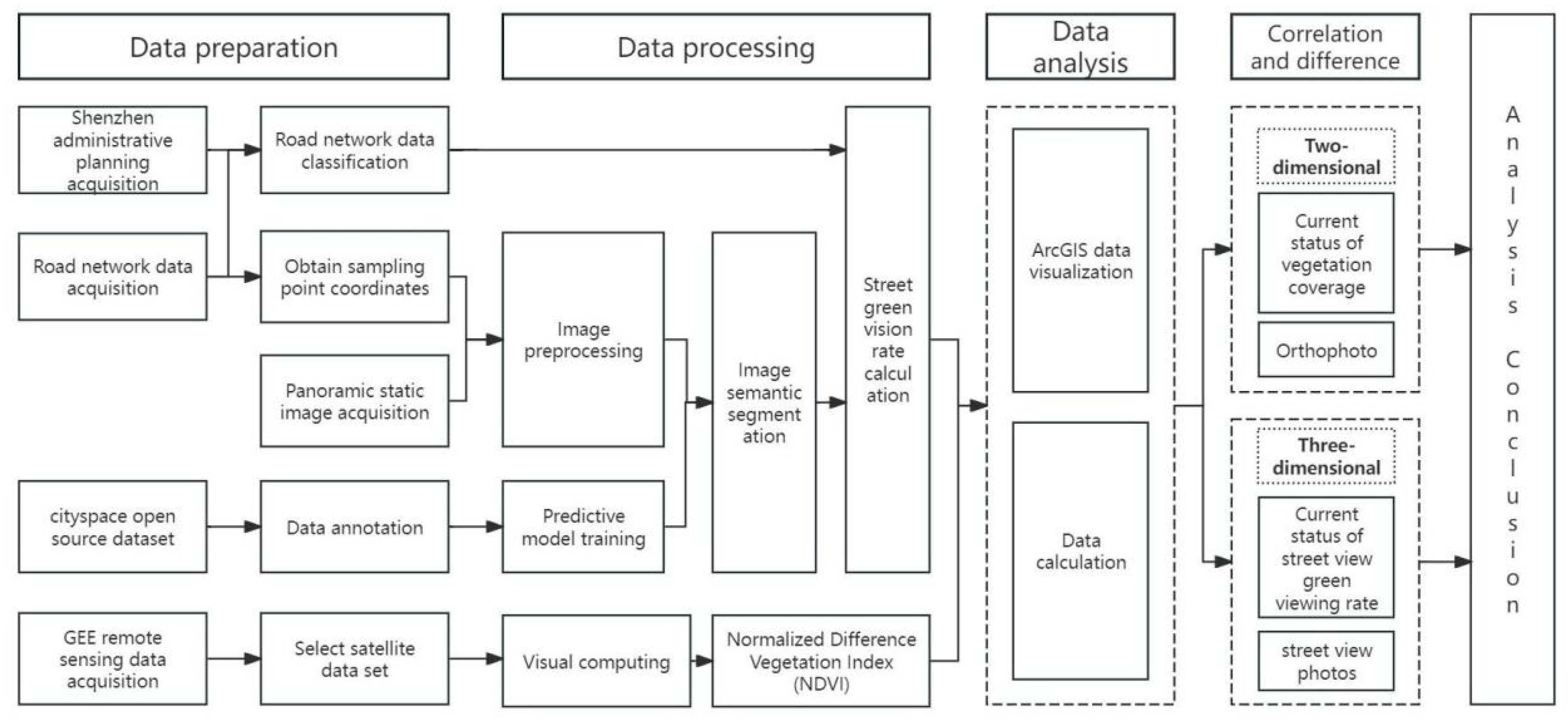
3.1. Analytical Framework

This study is based on Shenzhen’s road network data, utilizing ArcGIS equidistant segmentation technology to generate observation points and export their coordinates, in conjunction with Baidu Maps API to obtain panoramic street images of the observation points. Fully convolutional networks are used to perform semantic segmentation on each panoramic street image, obtaining the area ratio of each semantic object and calculating the street green view index. Finally, combined with the results measured by the Normalized Difference Vegetation Index, a two-dimensional and three-dimensional correlation analysis of the green spaces of Shenzhen’s streets is conducted.The technical path of this study is shown in Figure 4 below.

3.2. NDVI Calculation

NDVI, generally used to indicate vegetation coverage, ranges from [−1, 1], where negative values represent high-reflectance ground cover such as clouds, snow, and water, and positive values indicate vegetation cover, with values closer to 1 indicating greater vegetation coverage. The formula for calculating NDVI is as follows:
NDVI = NIR R NIR + R
In the formula, NIR (near infrared) represents the near-infrared band; R is the red band.
In practical applications, NDVI data may have null values, meaning some areas lack data, which can be due to various reasons: cloud cover and atmospheric particles (such as smoke and dust) can obscure the surface, preventing satellite images from capturing ground information, resulting in null values in NDVI calculations. Additionally, the strong red light absorption and weak near-infrared reflection by water bodies lead to extremely low NDVI values, which are sometimes erroneously processed as no data. Limitations in the resolution or detection capabilities of satellite sensors, especially for very small or narrow surface features, can also result in null values in NDVI maps. Seasonal changes in vegetation, such as dormancy in winter, can cause significant decreases in NDVI values, which, if not properly identified, may be mistakenly marked as no data.
To reduce errors and optimize data quality, we selected remote sensing images from five adjacent time periods with the least cloud cover for analysis. In the final raster calculation, the average of non-null values was used to ensure the accuracy and reliability of the NDVI results. Through spatial autocorrelation analysis of the data, a z-score of 406.189840901 (Figure 5) was obtained, indicating a less than 1% probability of this clustering pattern occurring by chance. The Moran index of 0.804601, close to 1, indicates a significant positive spatial autocorrelation in the analyzed features, meaning similar values tend to cluster in space. The p-value is zero, with a confidence level above 99%.

3.3. GVI Calculation

The GVI is a measure of the visible green vegetation area in a specific urban area or street, reflecting the level of greening in that area. Its core concept includes the ratio of the green vegetation area visible to the human eye within a certain range to the overall visible area. A higher GVI indicates better greening of the area.

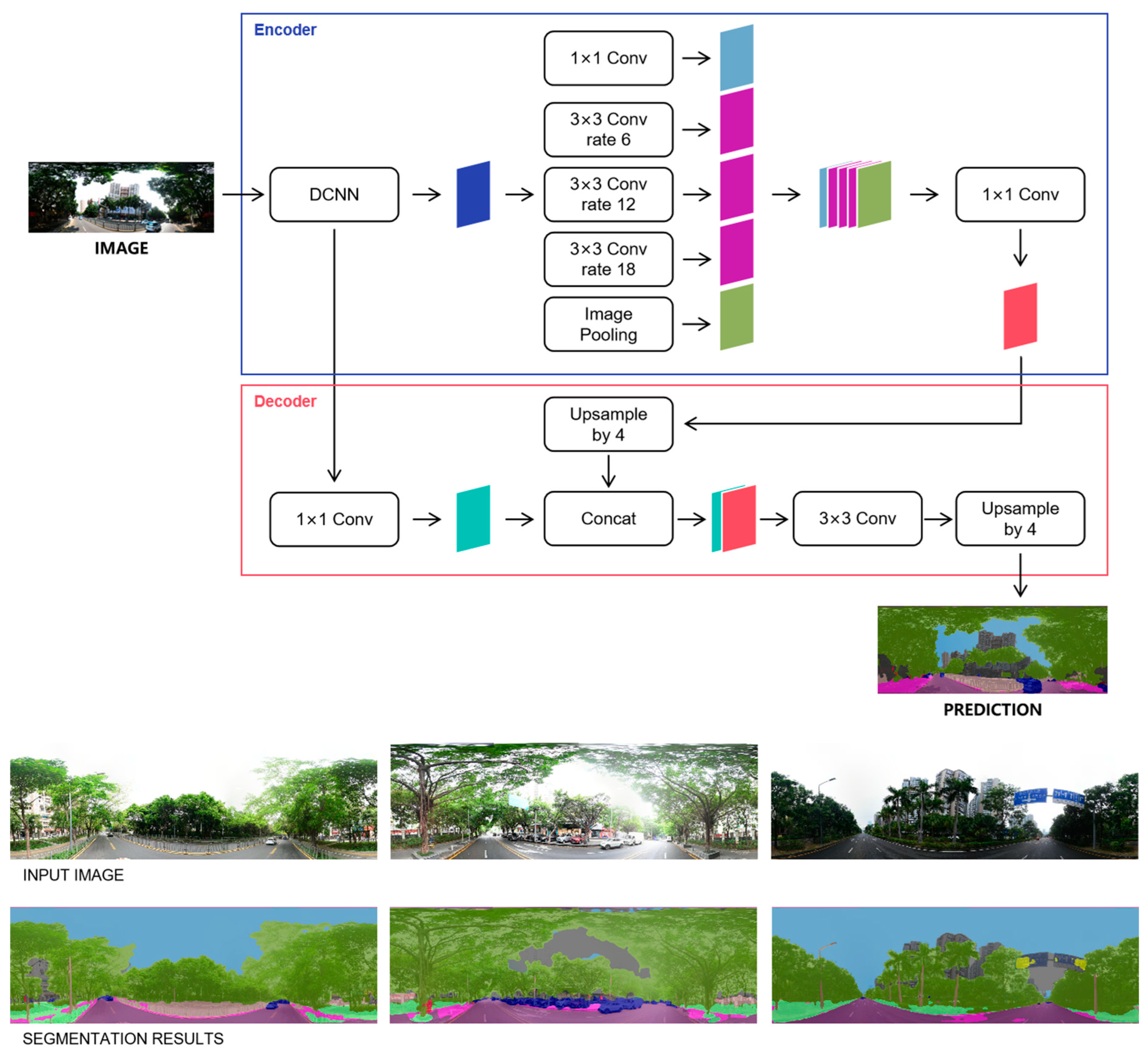
3.3.1. GVI Recognition Based on Image Semantic Segmentation Neural Network

The Convolutional Neural Network (CNN) is a deep learning model used for image and video analysis. It performs convolution operations on input data through convolutional kernels, automatically learning to extract spatial features from images, followed by pooling for dimensionality reduction and fully connected layers for classification, thus enabling tasks such as image classification, object detection, and semantic segmentation. CNNs have achieved excellent recognition performance and are now widely used in the fields of computer vision and image processing (Yao et al., 2019) [29]. The Deep Convolutional Neural Network (DCNN) gradually extracts increasingly abstract features through the combination of multiple convolutional and pooling layers, starting from simple edges to complex object parts, ultimately forming an understanding of the whole object. This characteristic of layer-by-layer extraction and abstraction makes DCNNs perform exceptionally well in image recognition tasks and they are now widely used in the fields of computer vision and image processing [30].
Cityscapes is a benchmark suite and dataset used for training and testing pixel-level and instance-level semantic segmentation. It consists of a large and diverse set of stereo video sequences recorded in 50 different city streets, providing high-quality pixel-level annotations and a large number of coarse annotations to be used for the recognition of various visual scenes [31].
The DeepLabV3+ segmentation model [32] is based on a Deep Convolutional Neural Network and extracts and restores semantic information of images through an encoder-decoder structure and ASPP (Atrous Spatial Pyramid Pooling). The encoder stage extracts contextual features, while the decoder addresses the problem of edge information loss. The detailed steps can be explained as follows (Figure 6): the Xception feature extraction network is used for feature extraction, generating two effective feature layers, namely shallow features and deep features; the extracted deep features are then input into the ASPP module, which includes a 1 × 1 convolution and three 3 × 3 convolutions with dilation rates of 6, 12, and 18, respectively. Different dilation rates are used in atrous convolutions to improve the receptive field of the network, giving the network different feature reception conditions. The ASPP layer compresses features through a 1 × 1 convolution, ultimately outputting the features captured by the entire encoder network. The shallow features generated by Xception enter the decoder, where multi-scale features are upsampled four times and then fused with the shallow features, followed by feature extraction using a 3 × 3 convolution. Finally, after four upsamplings, the output image matches the input image [33]. This model has outstanding performance in refining object boundary features and improving segmentation results [34].
In this study, the DeepLabV3+ segmentation model was used, trained on the CityScapes open-source dataset using PyTorch to obtain the final prediction model, which recognizes 19 classes of image content (Table 4).

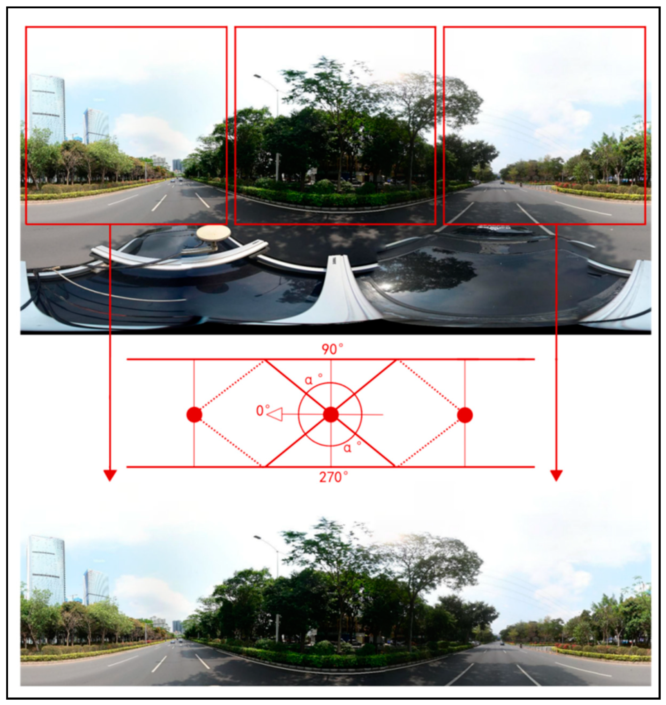
3.3.2. Minimizing Deformation Error

When capturing street panoramic images, the wide field of view of the camera and the need for image stitching to achieve panoramic effects can cause certain degrees of distortion and deformation at the top and bottom of the image. This distortion is primarily manifested as the elongation and thinning of object shapes, with a change in the size ratio between the top and bottom of the same object.
The deformation in panoramic images can have a negative impact on image semantic segmentation algorithms based on convolutional neural networks. This is because the convolutional kernel parameters in convolutional neural networks are typically learned based on the features of objects in normal proportions, and when objects in the image are distorted, their features undergo certain deviations. This reduces the network’s ability to recognize objects in distorted areas, leading to an increase in pixel-level misclassifications in the semantic segmentation results, especially for the top and bottom parts of the image. To improve the accuracy of semantic segmentation of panoramic images, modifications to the network structure are needed to accommodate the distortion in panoramic images, modeling the feature changes in the top and bottom areas to reduce the decrease in semantic segmentation accuracy caused by distortion.
To minimize errors, this study adopted the methods of Yin (2015) [35] and Ye (2019) [36] (Figure 7), cropping the central part of the panoramic image to better match the perspective of a normal pedestrian, more accurately reflecting the actual visual perception of urban street greening.
The semantic segmentation prediction model is used to calculate 14,264 processed panoramic street view images. The proportion of the vegetation area at each sampling point (Table 4) in the entire image is the GVI value of the point. The sampling point data are imported into ArcGIS, and combined with information such as administrative boundaries, the overall GVI score of different areas can be obtained.

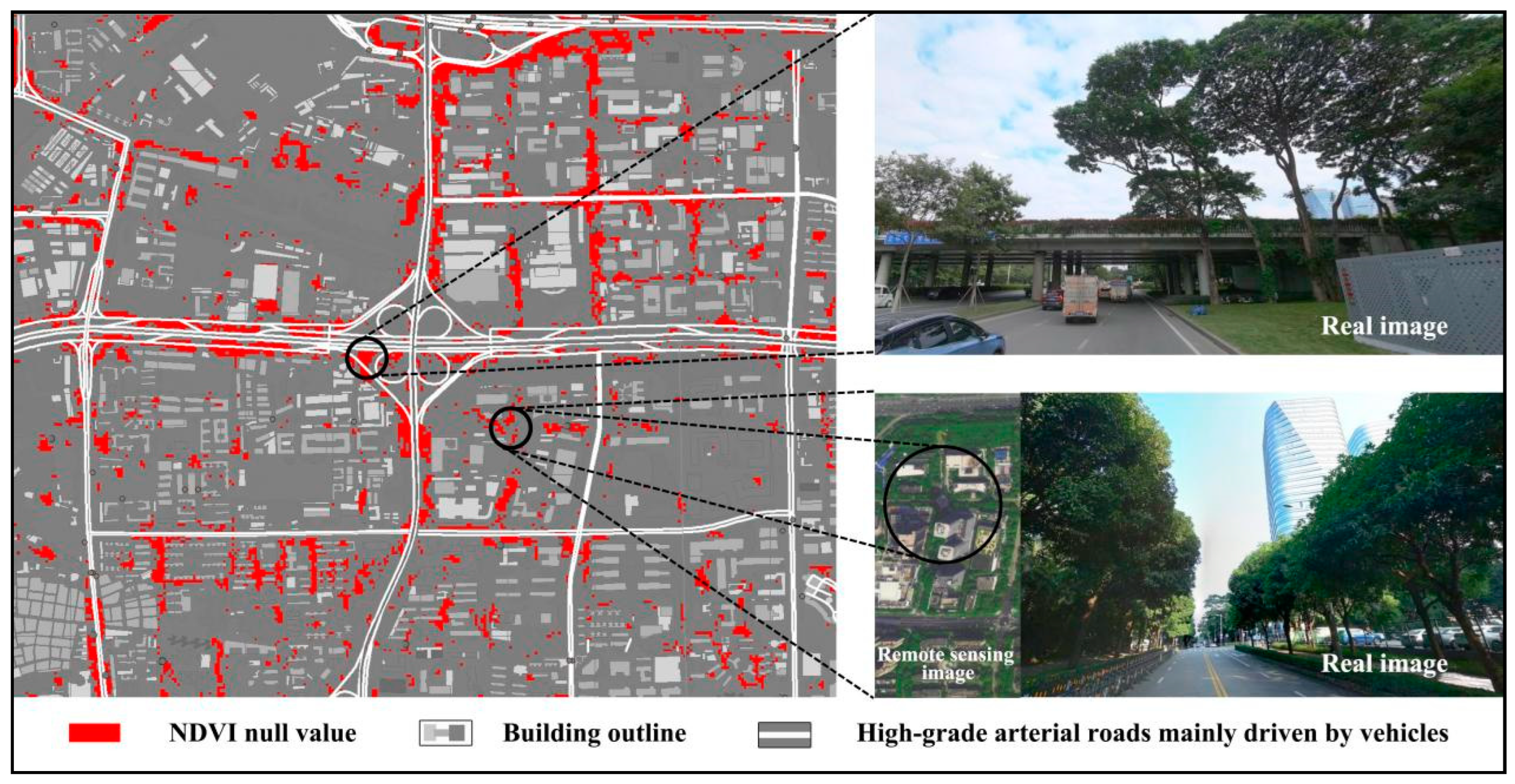
3.3.3. Reasons for the Null Value of GVI Data

As shown in the comparison in Figure 8, the 3D green space data contain many null values compared to the 2D data. This is because the street view map data used in this study were obtained through street view collection vehicles, which cannot collect Green View Index data for non-vehicular traffic areas. This means that GVI data for non-vehicular areas such as urban parks and residential communities were not captured in this study. For example, at the Shenzhen Golf Course (Figure 9), despite having extremely high greening coverage, the GVI values are almost blank because the sampling vehicle could not access these areas. Therefore, in this study, the correlation and difference analyses of the two-dimensional data were conducted based on the intersection of NDVI images and street view images.

4. Results and Discussion

4.1. Overall Characteristics of Street Green Spaces

4.1.1. In Three-Dimensional Space, the Road Greening Levels in Shenzhen’s Nanshan, Futian, and Luohu Districts Are Overall High

From the perspective of regional differences, this study compared the road greening conditions in Shenzhen’s three major urban districts: Nanshan, Futian, and Luohu. The research results (Table 5) indicate that the road green view rates in the Nanshan, Futian, and Luohu districts are similar, at 26.05, 25.82, and 26.51, respectively, all above 25%, indicating a level of “comfort”. The absolute difference between the average and median values is small, indicating an even distribution of data and no significant bias in green space resources.
Shenzhen’s main urban districts have a high level of road greening, with a wide coverage and overall balance. The image data used in this study were mainly collected in the summer, representing the vibrant summer scenery of Shenzhen’s road greening.

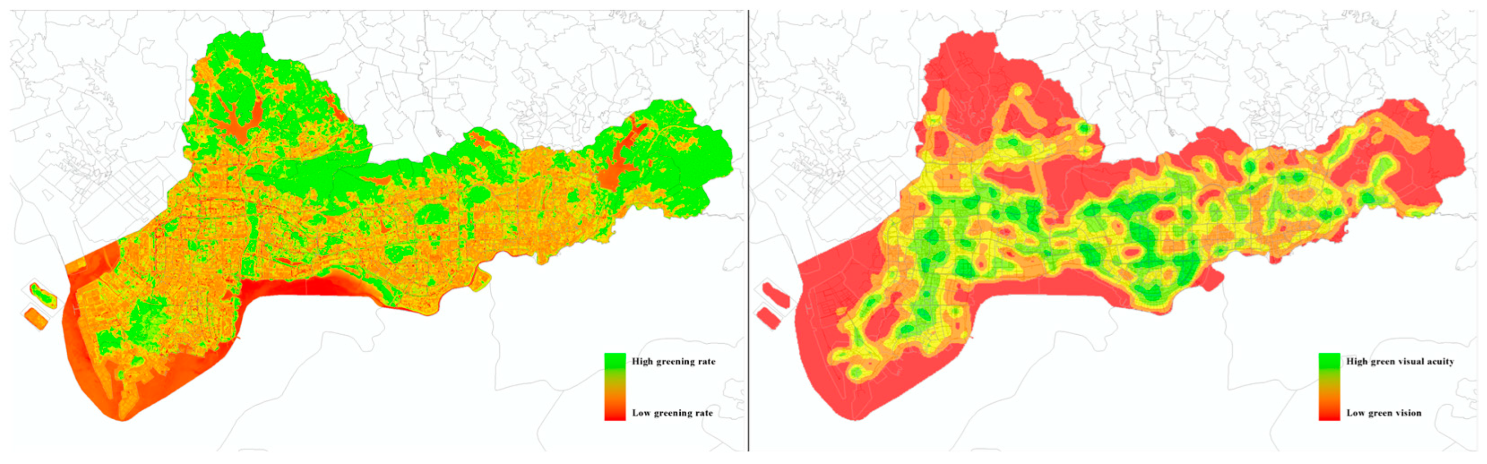
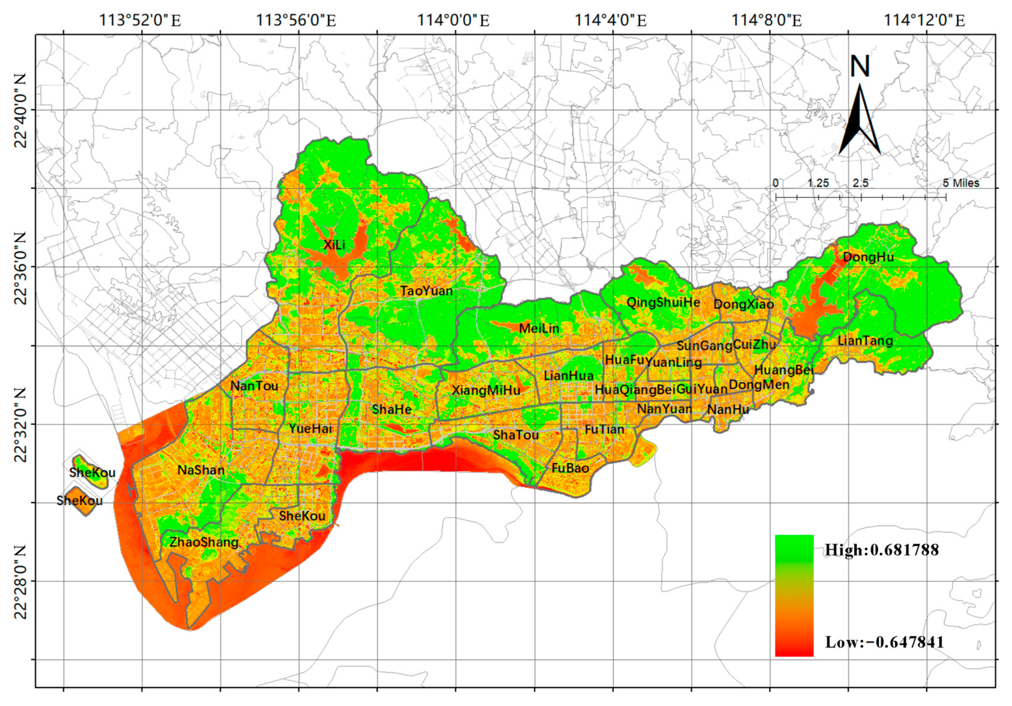
4.1.2. In Two-Dimensional Space, Urban and Forest Parks Form the Backbone, with Road Greening Connecting to Form a Green Ecological Network

Through detailed analysis of vegetation coverage, it was observed that despite the high urban development pressure, the core areas of Shenzhen still have generally high NDVI values (Figure 10), demonstrating significant success in urban greening. The region is scattered with parks and green spaces of various sizes, interconnected by meticulously designed road greenings, together forming a coherent green ecological network.

4.2. Correlation Analysis between Two-Dimensional and Three-Dimensional Street Green Space

To explore in depth the correlation and differences between three-dimensional blue-green spaces from a pedestrian’s perspective and two-dimensional vegetation coverage from an aerial perspective, this study extracted the NDVI and the corresponding GVI for each sampling point. During the extraction process, bilinear interpolation [37] was used to reduce errors, considering the potential influence of the surrounding environment.
The correlation between GVI and NDVI for the same sampling point was analyzed using Pearson’s correlation coefficient to study the relationship between street green spaces in two-dimensional and three-dimensional spaces. Pearson’s correlation coefficient ( r ) is calculated as the covariance of two variables divided by the product of their standard deviations.
r = n ( xy ) - ( x ) ( y ) [ n x 2 ( x ) 2 ] [ n y 2 ( y ) 2 ]
Through calculation and analysis, the Pearson correlation coefficient between GVI and NDVI was found to be 0.5818 (p < 0.001, where p represents the significance level), indicating a moderate level of correlation. The results highlight the inconsistency between remote sensing images and street view images in representing street green spaces.

4.3. Analysis of the Causes of Differences

Currently, scholars define the NDVI classification as follows: areas with less than 0.1 are non-vegetated; 0.1–0.3 are poorly vegetated; 0.3–0.6 are moderately vegetated; 0.6–0.8 are well vegetated; more than 0.8 are excellently vegetated [38,39]. However, this study found that these classification thresholds are too high and do not accurately reflect the level of vegetation cover in urban built-up areas, leading to a reclassification of the existing data levels. Ultimately, this study meticulously reclassified NDVI and GVI using the natural breaks method into five levels and further categorized into four typical greening scenarios (Table 6, Figure 11): high NDVI with high GVI, high NDVI with low GVI, low NDVI with high GVI, and low NDVI with low GVI. Of 14,264 valid sample points, 10,176 are in the range considered ideal for green view rate and vegetation coverage (NDVI values between 0.13 and 0.4, GVI values between 0.15 and 0.60), accounting for 71.34%. These data indicate that the core areas of Shenzhen have excelled in the construction of green infrastructure for roads, with significant overall planning and implementation effects.
The study analyzed the distribution and causes of four types of characteristics in two- and three-dimensional green infrastructure, with particular focus on areas with a notable contrast: those with low NDVI but high GVI, and those with high NDVI but low GVI. Through in-depth analysis of these special cases, the study aims to uncover the multidimensional characteristics of urban greening and the reasons behind their differences.

4.3.1. Areas with High NDVI and GVI and Their Main Causes

We overlaid the spatial distribution of sampling points with both high GVI and NDVI characteristics with the spatial distribution of urban parks, and found that the locations of these sampling points matched experimental expectations. The spatial locations of these characteristic sampling points highly coincide with the areas rich in vegetation in the core areas of Shenzhen in terms of spatial distribution (Figure 12).
Specifically, in the core areas of Shenzhen, sampling points with high GVI and NDVI values are mainly found in two types of areas: many such points are concentrated around urban parks like OCT National Park (Figure 13), Nanshan Park, Xiangmi Park, and Lianhua Mountain Park. Additionally, a few sampling points are located in non-park places with rich vegetation and good environments, such as Shenzhen University and Happy Valley (Figure 13). Both types of areas share the common features of having abundant greenery and a good ecological environment, with mature trees, making the green coverage not only rich from a horizontal perspective but also vibrant and diverse vertically. This three-dimensional greening structure ensures the coexistence of high GVI and NDVI values.

4.3.2. Areas with Low NDVI and GVI and Their Main Causes

Sampling points characterized by low NDVI and GVI also display a certain regularity in spatial distribution, primarily appearing in linear and clustered forms (Figure 14). Addressing this phenomenon, the study investigates from two perspectives: the reasons for the reduction in GVI and the causes of the decrease in NDVI. In analyzing GVI, to minimize the impact of semantic segmentation classification accuracy on the research findings, data from “wall” and “building” categories were combined into a “Building” category. Furthermore, the study filtered potential influencing factors for the GVI values of sampling points and conducted a correlation analysis on the sky retention rate, the proportion of roads in the line of sight, and the proportion of buildings in the line of sight. The analysis revealed a moderate negative correlation of −0.418 between Building and Vegetation (Table 7). Comparing panoramic static images of the area, we found that in areas with both low NDVI and GVI, the scant greenery between dense buildings is the main factor causing the reduction in GVI.
In the NDVI study, we also noticed that the number of low NDVI feature points exceeded expectations, such as the situation at the intersection of Nanhai Avenue and Beihuan Avenue in Figure 15. Upon further analysis of the data, a large number of null values were found. Detailed analysis of the photos of sampling points in these null areas, combined with research on urban roads and building heights, revealed that high-grade roads (especially overpasses) and buildings also have a significant negative impact on the calculation of NDVI values.
Based on the aforementioned analysis, we observed that areas around high-grade roads, primarily used for vehicular traffic, often exhibit low GVI and NDVI values. This phenomenon is mainly due to the wide roadways and complex three-dimensional traffic structures of high-grade roads, resulting in reduced green view rates and greening rates. On the other hand, areas adjacent to medium-grade roads, primarily used for vehicular traffic with pedestrian pathways on both sides, and low-grade roads, primarily used for pedestrian traffic, also commonly have low GVI and NDVI values. This is because the building heights and densities in these areas are too high and the roads are narrow, limiting the implementation of large-scale greening; thus, both the green view rate and greening rate are low.

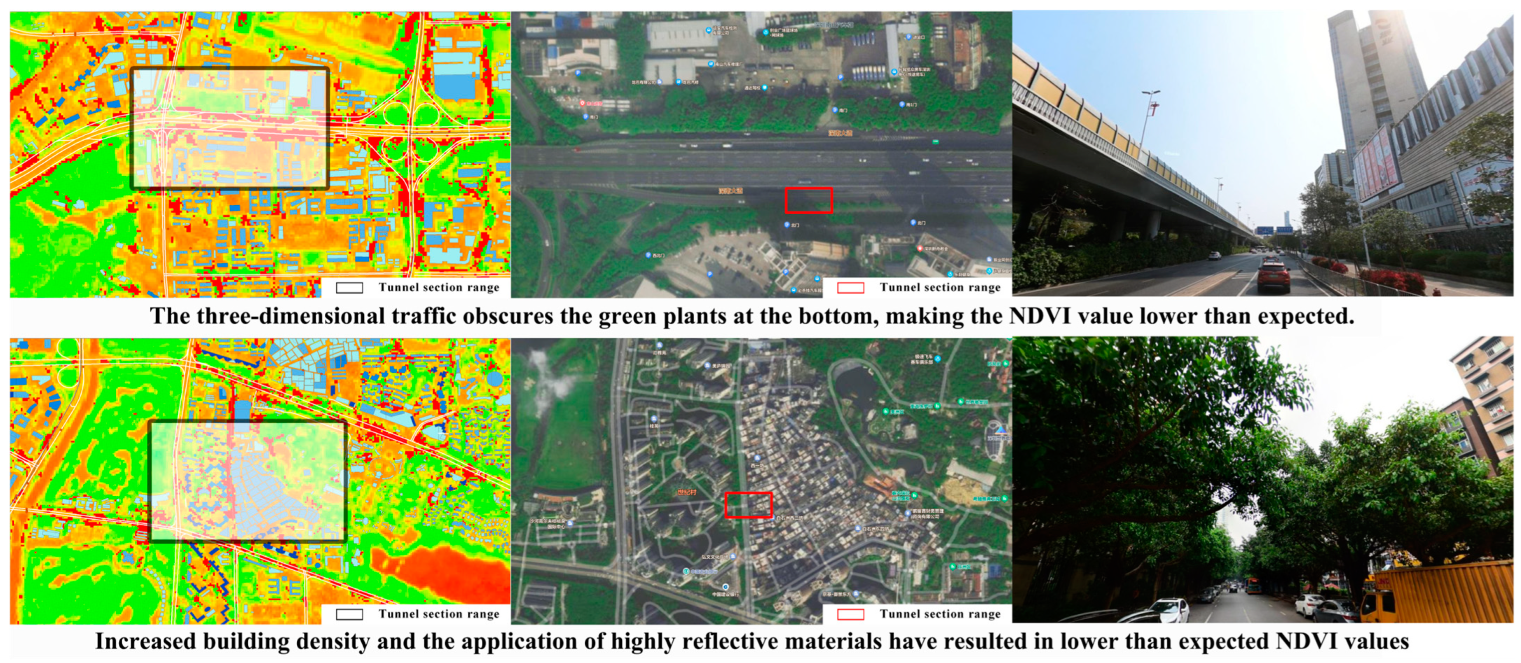
4.3.3. Areas with High NDVI but Low GVI and Their Main Causes

Three typical scenarios of high NDVI but low GVI features occur at some urban center intersections, specific tunnel sections, and certain road construction areas (Figure 16).
In some urban center intersections, low shrubs or lawns are often chosen for greening layouts to ensure traffic safety and clear visibility. Although such greening methods can maintain clear driving sightlines, the relatively sparse vegetation coverage results in lower GVI in these areas. However, due to Shenzhen’s sufficient emphasis on the design of green belts along roads, the NDVI values in these areas overall remain at a high level.
Another situation mainly occurs in tunnel sections like the Dongbin, Tanglangshan, and Henglongshan tunnels (Figure 17). In these areas, the misalignment between the sampling points of panoramic static images and the spatial locations represented by remote sensing images can lead to biased results. Remote sensing images capture the green areas on the mountaintops, leading to higher NDVI values, but the lack of vegetation inside the tunnels results in extremely low GVI values in these areas.
In special nodes of urban road construction areas, this result is also displayed: during construction, the green belts along the roads are often temporarily blocked or covered to ensure construction safety and convenience. This practical intervention inevitably affects the visibility and observability of vegetation, leading to significant spatial distribution inconsistencies between field observations and remote sensing image analysis. Although remote sensing images may show high vegetation coverage in the area, the green view rate observed on-site may be significantly reduced due to the obstruction of construction barriers. However, considering that the update interval of urban street view image data is long, the street construction time is generally short, and this type of feature points accounts for a small proportion of the overall number, this study maintains that the error caused by this situation will not have a decisive impact on the overall conclusion.

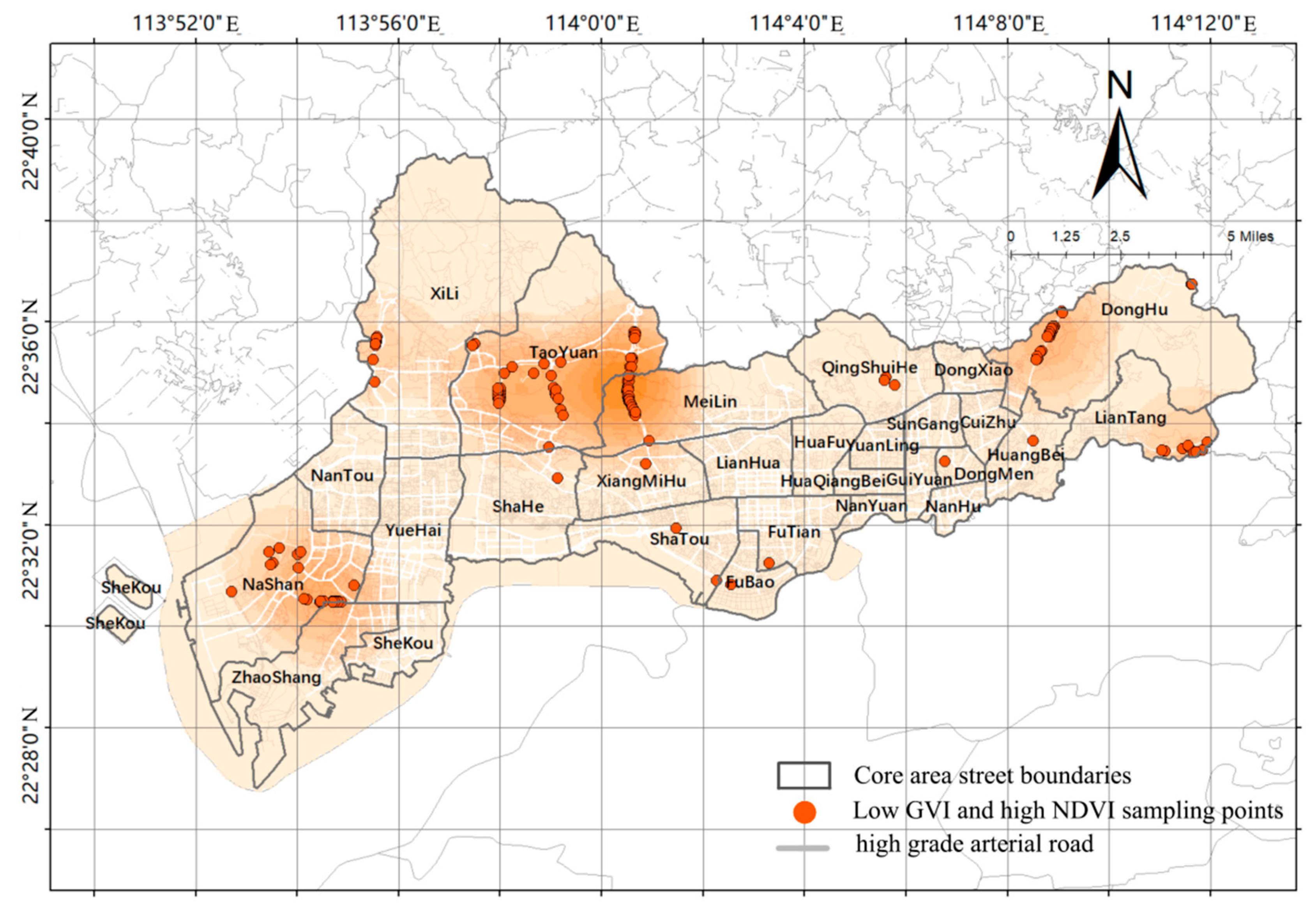
4.3.4. Areas with Low NDVI and High GVI and Their Main Causes

Through the analysis of the actual street view images of the difference points (Figure 18 and Figure 19), it is found that the phenomenon of low NDVI and high GVI is mainly classified into the following two reasons.
Firstly, the complexity of the three-dimensional traffic structure in the study area causes a disparity between the two indicators, with sampling points fitting this characteristic typically concentrated in areas with higher overpasses, such as Shennan Avenue and Beihuan Avenue. Although the greening work at the base of these overpasses has been adequately attended to and implemented, ensuring a suitable GVI range, the top structure of the overpasses obscures the underlying vegetation, resulting in NDVI values that do not accurately reflect the actual level of greening. This structural obstruction limits the satellite’s direct observation of ground vegetation, thus affecting the accurate calculation of NDVI.
Secondly, the core areas of Shenzhen have a generally high building density, intense urban development, and a modern architectural style, such as the Shenzhen High-Tech Industrial Park, representing high-tech industries, and Baishizhou Urban Village, known for its concentrated building density. This dense architectural layout poses a challenge to the resolution accuracy of remote sensing images, making it difficult for satellites to accurately identify green infrastructure around buildings. Moreover, the high-reflectance materials used on some building surfaces further increase the difficulty of remote sensing recognition, preventing the capture of valid vegetation information in these areas and resulting in null values. Thus, the combined effect of physical obstruction by buildings and the characteristics of high-reflectance surfaces also leads to NDVI values being lower than expected, and in some cases, data are missing.
The complexity of urban three-dimensional traffic structures, increased building density, and the high reflectivity of specific materials are key factors causing the significant discrepancy of low NDVI and high GVI. As evidenced by these findings, the impact of urban structure and material properties on remote sensing data must be taken into account when conducting urban vegetation monitoring and assessment to improve the accuracy and reliability of the data. Meanwhile, in terms of optimizing urban green landscapes, adopting multi-level greening methods and increasing street green spaces are good ways to improve urban vegetation coverage and the quality of green spaces. Multi-level greening methods require maximizing green coverage not only on the ground but also on building roofs, building facades, and around roads, giving urban residents more opportunities to interact with natural vegetation. Increasing street green spaces requires cities to find every possible piece of land in densely built areas that can be used for green space construction.

4.4. Discussion

Does “the tree by the roadside” represent the same information in the eyes of planners and residents?
In recent years, scholars have noticed various urban spatial data such as GVI and NDVI when evaluating and perceiving urban green spaces, and have recognized the differences between them, applying these insights to their own related research. In this era of information technology explosion, research using data as a tool to understand cities has made significant progress, enabling solutions to problems that were previously unsolvable. Examples include using nighttime light images and deep learning to classify land cover [28], summarizing global air pollution trends over a 20-year period [40], and using convolutional neural networks to detect objects on roads [41]. Relevant research has also gradually entered a period of rapid development.
The current mainstream direction is towards “big” data, and large datasets often tend to overlook the precision of details. A considerable number of studies have pointed out the limitations of different big datasets. For instance, Huang, S. et al. [42,43,44] identified atmospheric effects, saturation phenomena, and sensor factors as major limitations in the application of NDVI; Zhou et al. [45,46] pointed out the issues of POI data sparsity, timeliness, and cold start; Huang et al. [47,48,49] highlighted problems such as the positional uncertainty of mobile signaling data, poor data coverage, and data noise. When conducting research at the urban scale, the limitations of datasets have a relatively small impact on the final results. However, when the research scale is reduced to the neighborhood level, the inherent limitations of the datasets can significantly affect the research outcomes.
Taking this study of urban street green space as an example, researchers have pointed out the limitations of NDVI under atmospheric conditions [50] and its difficulty in identifying vegetation [51], but they have not delved into the specific feedback of NDVI at the urban street scale. At this scale, can planners still see “the tree by the roadside”?
This study attempts to use GVI and NDVI data as case studies to explore the correlation and differences between them, and to summarize the real-world manifestations of numerical anomalies. The aim of the research is to use real-world cases as intermediaries to find the mapping relationships between different types and dimensions of data in reality, and to attempt to extend this experience to other datasets. In this way, scholars’ research will no longer isolate data into different research systems, but instead will attempt to reveal the intrinsic connections between data. Additionally, this study aims to enable planners, when facing various spatial data, to go beyond a purely “God’s perspective” and avoid the inherent limitations of the datasets. By understanding the intrinsic connections between data, planners can align their perceptions with residents’ actual experiences.

5. Conclusions

5.1. Main Findings

5.1.1. Shenzhen’s Core Area Has Good Green Infrastructure Construction

This study focuses on the road greening conditions in Nanshan District, Futian District, and Luohu District of Shenzhen, and finds that the GVI of roads in these three areas is above 25%. The distribution of green space is relatively balanced, showing a high level of greening. Especially in Nanshan District, which is one of the most modernized areas in Shenzhen, the GVI is the highest. This indicates that modern urban construction in China increasingly emphasizes the creation of green spaces. Additionally, by classifying the NDVI and GVI of 14,264 valid sampling points, it is found that over 70% of the sample points are in the ideal range for both GVI and vegetation coverage, indicating that Shenzhen has achieved significant success in road greening and green infrastructure construction.

5.1.2. Moderate Correlation between 2D and 3D Greening Data

A comparative analysis of the NDVI and GVI indices at the sampling points revealed a moderate correlation between these two indicators. This result highlights the potential differences in observing green spaces from different perspectives (2D and 3D) and indicates that visible green space does not necessarily equate to actual green space.

5.1.3. Four Classification Relationships between 2D and 3D Greening Data

The study further explored four typical greening scenarios: high NDVI and high GVI, high NDVI and low GVI, low NDVI and high GVI, and low NDVI and low GVI. We found that areas with high NDVI and high GVI are mainly distributed in vegetation-rich areas such as urban parks. The greening structures in these areas perform well both horizontally and vertically, making the greening levels consistent between remote sensing images and actual perceptions. In contrast, areas with low NDVI and low GVI are usually located between dense buildings or in areas affected by overpasses and structures, where these factors limit the implementation of greening and the accuracy of remote sensing data.

5.1.4. The Limitation of the Sampler’s Perspective Is the Main Cause of Differences between 2D and 3D Green Space Data

Additionally, we focused on analyzing the discrepancies between “what is seen” and “what is measured”: areas with high NDVI but low GVI mainly appear at traffic intersections and tunnel sections in urban centers. The greening layout in these areas is influenced by traffic safety or construction activities, with factors such as mountains above tunnels blocking satellite views and construction enclosures blocking the street view sampling vehicle’s perspective, resulting in remote sensing observations being higher than the actual green space. On the other hand, areas with low NDVI but high GVI are mainly due to the impact of three-dimensional traffic structures and high-density buildings on remote sensing images, which prevent remote sensing images from accurately capturing pedestrian perceptions from an overhead perspective. These factors cause NDVI values to be lower than the greening level actually perceived by residents in their daily lives.

5.1.5. Using GVI as a Substitute for NDVI Null Values Can Reduce Greening Assessment Errors

Regarding the accuracy and reliability of remote sensing monitoring, this study indicates that in urban environments, the height, density, material of buildings, and elevated transportation facilities can significantly interfere with the measurement of vegetation indices, thereby affecting the accuracy of NDVI. Therefore, when using NDVI to analyze the greening level of urban built-up areas, researchers need to pay close attention to the null values of NDVI and consider using GVI as a supplement to represent the greening level of the corresponding area. This method can further improve the accuracy of research and ensure a more precise and comprehensive assessment of urban greening conditions.

5.2. Limitations

There are still some limitations in this research, which need to be further studied in the future. Firstly, in this study, the collection points of street panorama images were limited and could not fully represent the entire greening situation of the road segments. The collected sample images could only reflect the local greening coverage of the road segment and could not fully reflect the overall greening level of the road segment. Therefore, there may be some discrepancies between the study results and the actual greening perceptions of the residents in the area. Future research should prioritize comparing residents’ perceptions of green spaces with the research results to address these discrepancies. Increasing the number of sampling points or reducing the time interval for data updates may improve the representativeness and accuracy of the results. Secondly, the image semantic segmentation approach used in this study also introduces errors due to the inherent misrecognition rate of the algorithm. The accuracy of the semantic segmentation algorithm, influenced by factors such as training data, cannot reach 100%, which affects the final green view index statistics. How to improve the robustness of segmentation algorithms is a direction that requires further research. Thirdly, the panoramic image samples in this study were limited and mainly collected from major streets in Shenzhen’s Nanshan, Luohu, and Futian districts. Consequently, the conclusions of this study can only represent the green view rate levels of these three districts during the summer, and the sample size is insufficient to generalize to other seasons or the entire city’s greening coverage. Fourthly, since the road surface occupies a large proportion in the vehicle-mounted perspective, and the greenery on both sides of the road takes up a relatively small portion of the field of view, this differs from the perspective of residents in their daily observations. The surrounding moving vehicles may also further obstruct the green view, affecting the actual perception of green spaces.

Author Contributions

Conceptualization, H.C. and C.Z; methodology, X.J.; investigation, X.J. and Z.L.; visualization, X.J. and Z.L.; writing—original draft preparation, X.J. and Z.L.; writing—review and editing, H.C., X.J., and C.Z.; supervision, H.C.; funding acquisition, H.C. All authors have read and agreed to the published version of the manuscript.

Funding

This research was funded by the National Natural Science Foundation of China, grant number 52378062.

Data Availability Statement

The data presented in this study are available upon request from the corresponding author.

Conflicts of Interest

The authors declare no conflicts of interest.

References

  1. National Bureau of Statistics of China. Annual Data of Major Economic Indicators of China. National Bureau of Statistics of China. 2024. Available online: https://data.stats.gov.cn/easyquery.htm?cn=C01 (accessed on 9 December 2023).
  2. Chen, Y.; Qiao, Y.; Yan, P.; Lu, H.; Yang, L.; Xia, J. Spatial-temporal variation and nonlinear prediction of environmental footprints and comprehensive environmental pressure in urban agglomerations. J. Clean. Prod. 2022, 351, 131556. [Google Scholar] [CrossRef]
  3. Liang, L.; Chen, M.; Lu, D. Revisiting the relationship between urbanization and economic development in China since the reform and opening-up. Chin. Geogr. Sci. 2022, 32, 1–15. [Google Scholar] [CrossRef]
  4. Herzog, T.R.; Gale, T.A. Preference for urban buildings as a function of age and nature context. Environ. Behav. 1996, 28, 44–72. [Google Scholar] [CrossRef]
  5. Gao, M.; Ahern, J.A.; Koshland, C.P. Perceived built environment and health-related quality of life in four types of neighborhoods in Xi’an, China. Health Place 2016, 39, 110–115. [Google Scholar] [CrossRef]
  6. Liu, Y.; Li, H.; Li, W.; Wang, S. Renovation priorities for old residential districts based on resident satisfaction: An application of asymmetric impact-performance analysis in Xi’an, China. PLoS ONE 2021, 16, e0254372. [Google Scholar] [CrossRef] [PubMed]
  7. Bahrainy, H.; Khosravi, H. The impact of urban design features and qualities on walkability and health in under-construction environments: The case of Hashtgerd New Town in Iran. Cities 2013, 31, 17–28. [Google Scholar] [CrossRef]
  8. Ji, J.S.; Chen, R.; Zhao, B. Megacity, Microscale Livable Space, and Major Depression. JAMA Netw. Open 2021, 4, e2130941. [Google Scholar] [CrossRef]
  9. Zeng, P.; Wei, X.; Duan, Z. Coupling and coordination analysis in urban agglomerations of China: Urbanization and ecological security perspectives. J. Clean. Prod. 2022, 365, 132730. [Google Scholar] [CrossRef]
  10. Zamparas, M.; Kyriakopoulos, G.L.; Drosos, M.; Kapsalis, V.C.; Kalavrouziotis, I.K. Novel composite materials for lake restoration: A new approach impacting on ecology and circular economy. Sustainability 2020, 12, 3397. [Google Scholar] [CrossRef]
  11. Kondo, M.C.; Fluehr, J.M.; McKeon, T.; Branas, C.C. Urban green space and its impact on human health. Int. J. Environ. Res. Public Health 2018, 15, 445. [Google Scholar] [CrossRef]
  12. Gao, Z.; Zaitchik, B.F.; Hou, Y.; Chen, W. Toward park design optimization to mitigate the urban heat Island: Assessment of the cooling effect in five US cities. Sustain. Cities Soc. 2022, 81, 103870. [Google Scholar] [CrossRef]
  13. Norton, B.A.; Coutts, A.M.; Livesley, S.J.; Harris, R.J.; Hunter, A.M.; Williams, N.S.G. Planning for cooler cities: A framework to prioritise green infrastructure to mitigate high temperatures in urban landscapes. Landsc. Urban Plan. 2015, 134, 127–138. [Google Scholar] [CrossRef]
  14. Farinmade, A.; Soyinka, O.; Siu, K.W.M. Assessing the effect of urban informal economic activity on the quality of the built environment for sustainable urban development in Lagos, Nigeria. Sustain. Cities Soc. 2018, 41, 13–21. [Google Scholar] [CrossRef]
  15. Sharifi, A. Co-benefits and synergies between urban climate change mitigation and adaptation measures: A literature review. Sci. Total Environ. 2021, 750, 141642. [Google Scholar] [CrossRef] [PubMed]
  16. Meerow, S.; Newell, J.P.; Stults, M. Defining urban resilience: A review. Landsc. Urban Plan. 2016, 147, 38–49. [Google Scholar] [CrossRef]
  17. Lu, Y.; Sarkar, C.; Xiao, Y. The effect of street-level greenery on walking behavior: Evidence from Hong Kong. Soc. Sci. Med. 2018, 208, 41–49. [Google Scholar] [CrossRef] [PubMed]
  18. Wolf, K.L. Business district streetscapes, trees, and consumer response. J. For. 2005, 103, 396–400. [Google Scholar] [CrossRef]
  19. Helbich, M.; Yao, Y.; Liu, Y.; Zhang, J.; Liu, P.; Wang, R. Using deep learning to examine street view green and blue spaces and their associations with geriatric depression in Beijing, China. Environ. Int. 2019, 126, 107–117. [Google Scholar] [CrossRef]
  20. Bell, S. Health and well-being aspects of urban blue space: The new urban landscape research field. Landsc. Archit. 2019, 26, 119–131. [Google Scholar]
  21. Aoki, Y. Relationship between perceived greenery and width of visual fields. J. Jpn. Inst. Landsc. Arch. 1987, 51, 1–10. [Google Scholar]
  22. Catania, J.A.; McDermott, L.J.; Pollack, L.M. Questionnaire response bias and face-to-face interview sample bias in sexuality research. J. Sex Res. 1986, 22, 52–72. [Google Scholar] [CrossRef]
  23. Li, X.; Zhang, C.; Li, W.; Ricard, R.; Meng, Q.; Zhang, W. Assessing street-level urban greenery using Google Street View and a modified green view index. Urban For. Urban Green. 2015, 14, 675–685. [Google Scholar] [CrossRef]
  24. Lu, Y. The association of urban greenness and walking behavior: Using google street view and deep learning techniques to estimate residents’ exposure to urban greenness. Int. J. Environ. Res. Public Health 2018, 15, 1576. [Google Scholar] [CrossRef] [PubMed]
  25. Kameoka, T.; Uchida, A.; Sasaki, Y.; Ise, T. Assessing streetscape greenery with deep neural network using Google Street View. Breed. Sci. 2022, 72, 107–114. [Google Scholar] [CrossRef] [PubMed]
  26. Chiang, Y.C.; Liu, H.H.; Li, D.; Ho, L.C. Quantification through deep learning of sky view factor and greenery on urban streets during hot and cool seasons. Landsc. Urban Plan. 2023, 232, 104679. [Google Scholar] [CrossRef]
  27. Shenzhen Bureau of Statistics. Shenzhen Statistical Yearbook 2023. National Bureau of Statistics of China. 2024. Available online: https://tjj.sz.gov.cn/gkmlpt/content/11/11182/post_11182604.html#4219 (accessed on 12 April 2024).
  28. Goldblatt, R.; Stuhlmacher, M.F.; Tellman, B.; Clinton, N.; Hanson, G.; Georgescu, M.; Wang, C.; Serrano-Candela, F.; Khandelwal, A.K.; Cheng, W.H.; et al. Using Landsat and nighttime lights for supervised pixel-based image classification of urban land cover. Remote Sens. Environ. 2018, 205, 253–275. [Google Scholar] [CrossRef]
  29. Yao, Y.; Liang, Z.; Yuan, Z.; Liu, P.; Bie, Y.; Zhang, J.; Wang, R.; Wang, J.; Guan, Q. A human-machine adversarial scoring framework for urban perception assessment using street-view images. Int. J. Geogr. Inf. Sci. 2019, 33, 2363–2384. [Google Scholar] [CrossRef]
  30. Zeiler, M.D.; Fergus, R. Visualizing and understanding convolutional networks. In Proceedings of the European Conference on Computer Vision, Zurich, Switzerland, 6–12 September 2014; pp. 818–833. [Google Scholar]
  31. Cordts, M.; Omran, M.; Ramos, S.; Rehfeld, T.; Enzweiler, M.; Benenson, R.; Franke, U.; Roth, S.; Schiele, B. The Cityscapes Dataset for semantic urban scene understanding. In Proceedings of the 2016 IEEE Conference on Computer Vision and Pattern Recognition (CVPR), Las Vegas, NV, USA, 27–30 June 2016; pp. 3213–3223. [Google Scholar]
  32. Du, S.; Liu, B.; Zhang, X. Incorporating DeepLabv3+ and object-based image analysis for semantic segmentation of very high resolution remote sensing images. Int. J. Digit. Earth 2021, 14, 357–378. [Google Scholar] [CrossRef]
  33. Chen, L.C.; Zhu, Y.; Papandreou, G.; Schroff, F.; Adam, H. Encoder-decoder with atrous separable convolution for semantic image segmentation. In Proceedings of the European Conference on Computer Vision (ECCV) 2018, Munich, Germany, 8–14 September 2018; pp. 801–818. [Google Scholar]
  34. Chen, L.C.; Papandreou, G.; Kokkinos, I.; Murphy, K.; Yuille, A.L. Semantic image segmentation with deep convolutional nets and fully connected CRFs. arXiv 2014, arXiv:1412.7062. [Google Scholar]
  35. Yin, L.; Cheng, Q.; Wang, Z.; Shao, Z. ‘Big data’ for pedestrian volume: Exploring the use of Google Street View images for pedestrian counts. Appl. Geogr. 2015, 63, 337–345. [Google Scholar] [CrossRef]
  36. Ye, Y.; Richards, D.; Lu, Y.; Song, X.; Zhuang, Y.; Zeng, W.; Zhong, T. Measuring daily accessed street greenery: A human-scale approach for informing better urban planning practices. Landsc. Urban Plan. 2019, 191, 103434. [Google Scholar] [CrossRef]
  37. Chao, L.; Zhang, K.; Li, Z.; Zhu, Y.; Wang, J.; Yu, Z. Geographically weighted regression based methods for merging satellite and gauge precipitation. J. Hydrol. 2018, 558, 275–289. [Google Scholar] [CrossRef]
  38. Wang, X.; Jiang, D.; Ma, D. Spatial auto-correlation analysis of vegetation cover using MODIS NDVI time series data: Regional comparison of Shandong Peninsula and Liaodong Peninsula. J. Arid Land Resour. Environ. 2013, 27, 139–144. [Google Scholar]
  39. Li, M.; Hou, X.; Ying, L.; Lu, X.; Zhu, M. Spatial-temporal dynamics of NDVI and its response to temperature and precipitation in the Yellow River Delta during the period 1998–2008. Resour. Sci. 2011, 33, 322–327. [Google Scholar]
  40. Sicard, P.; Agathokleous, E.; Anenberg, S.C.; De Marco, A.; Paoletti, E.; Calatayud, V. Trends in urban air pollution over the last two decades: A global perspective. Sci. Total Environ. 2023, 858, 160064. [Google Scholar] [CrossRef] [PubMed]
  41. Bai, Y.; Shang, C.; Li, Y.; Shen, L.; Jin, S.; Shen, Q. Transport object detection in street view imagery using decomposed convolutional neural networks. Mathematics 2023, 11, 3839. [Google Scholar] [CrossRef]
  42. Huang, S.; Tang, L.; Hupy, J.P.; Wang, Y.; Shao, G. A commentary review on the use of normalized difference vegetation index (NDVI) in the era of popular remote sensing. J. For. Res. 2021, 32, 1–6. [Google Scholar] [CrossRef]
  43. Calota, I.; Faur, D.; Datcu, M. Estimating NDVI from SAR Images Using DNN. In Proceedings of the IGARSS 2022—2022 IEEE International Geoscience and Remote Sensing Symposium 2022, Kuala Lumpur, Malaysia, 17–22 July 2022; pp. 5232–5235. [Google Scholar]
  44. Rao, Y.; Zhu, X.; Chen, J.; Wang, J. An Improved Method for Producing High Spatial-Resolution NDVI Time Series Datasets with Multi-Temporal MODIS NDVI Data and Landsat TM/ETM+ Images. Remote Sens. 2015, 7, 7865–7891. [Google Scholar] [CrossRef]
  45. Xu, C.; Ding, A.; Zhao, K. A novel POI recommendation method based on trust relationship and spatial-temporal factors. Electron. Commer. Res. Appl. 2021, 48, 101060. [Google Scholar]
  46. Zhou, M.; Wang, M.; Hu, Q. A POI data update approach based on Weibo check-in data. In Proceedings of the 2013 21st International Conference on Geoinformatics 2013, Kaifeng, China, 20–22 June 2013; pp. 1–4. [Google Scholar]
  47. Huang, Q.; Yang, Y.; Xu, Y.; Yang, F.; Yuan, Z.; Sun, Y. Citywide road-network traffic monitoring using large-scale mobile signaling data. Neurocomputing 2021, 444, 136–146. [Google Scholar] [CrossRef]
  48. Xu, Y.; Li, X.; Shaw, S.; Lu, F.; Yin, L.; Chen, B. Effects of Data Preprocessing Methods on Addressing Location Uncertainty in Mobile Signaling Data. Ann. Am. Assoc. Geogr. 2020, 111, 515–539. [Google Scholar] [CrossRef]
  49. Gang, H.; Fu, L.; Liu, C.; Shen, Z. Using Massive Mobile Signaling to Monitor the Highway Traffic. In Signal and Information Processing, Networking and Computers, Proceedings of the 4th International Conference on Signal and Information Processing, Networking and Computers (ICSINC), Qingdao, China, 23–25 May 2019; Springer: Singapore, 2019; pp. 221–228. [Google Scholar]
  50. Li, F.; Han, L.; Zhu, L.; Huang, Y.; Song, G. Urban vegetation mapping based on the hj-1 ndvi reconstruction. ISPRS-Int. Arch. Photogramm. Remote Sens. Spat. Inf. Sci. 2016, 41, 867–871. [Google Scholar] [CrossRef]
  51. Martinez, A.; Labib, S. Demystifying normalized difference vegetation index (NDVI) for greenness exposure assessments and policy interventions in urban greening. Environ. Res. 2022, 220, 115155. [Google Scholar] [CrossRef] [PubMed]
Figure 1. Location map of the study area.
Forests 15 00983 g001
Figure 2. Image map of the study area.
Forests 15 00983 g002
Figure 3. Distribution of sampling points in the study area.
Forests 15 00983 g003
Figure 4. Research technology path.
Forests 15 00983 g004
Figure 5. Spatial autocorrelation and clustering difference analysis.
Forests 15 00983 g005
Figure 6. Schematic diagram of DeepLabV3+ network structure and segmentation results.
Forests 15 00983 g006
Figure 7. Panoramic static image deformation prevention processing method.
Forests 15 00983 g007
Figure 8. Comparison of two-dimensional green space (left) and three-dimensional green space (right) in Shenzhen.
Forests 15 00983 g008
Figure 9. GVI data missing due to the sampling vehicle being unable to enter the golf course.
Forests 15 00983 g009
Figure 10. Overall vegetation coverage in the core area.
Forests 15 00983 g010
Figure 11. Distribution diagram of four types of green infrastructure characteristics.
Forests 15 00983 g011
Figure 12. “NDVI high GVI high” feature sampling point distribution.
Forests 15 00983 g012
Figure 13. Example of distribution of characteristic sampling points of “high NDVI and high GVI”.
Forests 15 00983 g013
Figure 14. “NDVI low GVI low” feature sampling point distribution.
Forests 15 00983 g014
Figure 15. NDVI null value distribution at the intersection of Nanhai Avenue and Beihuan Avenue.
Forests 15 00983 g015
Figure 16. “NDVI high GVI low” feature sampling point distribution.
Forests 15 00983 g016
Figure 17. “NDVI high GVI low” characteristic sampling points represented by tunnel sections.
Forests 15 00983 g017
Figure 18. “NDVI low GVI high” feature sampling point distribution.
Forests 15 00983 g018
Figure 19. A large number of three-dimensional traffic and excessive building density in the core area make the NDVI value lower than expected.
Forests 15 00983 g019
Table 1. Statistical Table of Basic Natural Information of Shenzhen, Guangdong Province, China (Shenzhen Bureau of Statistics, 2024) [27].
Climate ElementsNatural Vegetation TypesLand Use Information
Average temperature (°C)23.3Percentage of subtropical and tropical evergreen broad-leaved and deciduous broad-leaved shrubs (%)64.59%Cultivated land (%)5.95%
Relative humidity (%)74Percentage of tropical mangroves (%)0.78%Forest land (%)29.14%
Precipitation (mm)1932.9Percentage of cultivated vegetation (artificial turf, artificial forests) (%)25.29%Grassland (%)1.23%
Sunshine hours (h)1853.0Percentage of subtropical coniferous forests (%)8.56%Water area (%)3.95%
High temperature days (d)4.4Percentage of subtropical and tropical grasses (%)0.78%Urban construction land (%)59.73%
Table 2. Statistics of land use information in Shenzhen, Guangdong Province, China (Shenzhen Bureau of Statistics, 2024) [27].
Land Type RatioShenzhenNanshanFutianLuohu
Arable land (%)5.958.770.764.73
Woodland (%)29.1424.6318.0649.10
Grassland (%)1.231.860.241.03
Waters (%)3.953.054.215.64
Urban construction land (%)59.7361.7076.7339.50
Table 3. Summary of data sources for application data.
No. Data NameData Source
1Population dataShenzhen Statistical Yearbook 2023 [27]
2GDP dataShenzhen Statistical Yearbook 2023 [27]
3Urbanization rate dataShenzhen Statistics Bureau
4Climate element informationShenzhen Statistics Bureau
5Natural vegetation type“1:1,000,000” China Vegetation Atlas
6Land use informationChinese Academy of Sciences Resource and Environmental Science Data Center
7Administrative divisionOpen Street Map
8Road informationOpen Street Map
9Panoramic static imageBaidu Map Open Platform
10Normalized difference vegetation indexGoogle Earth Engine
Table 4. Semantic segmentation categories.
NumberSemantic Segmentation Categories10Terrain
1road11sky
2sidewalk12person
3building13rider
4wall14car
5fence15truck
6pole16bus
7traffic light17train
8traffic sign18motorcycle
9vegetation19bicycle
Table 5. Statistics of green vision rate in three districts of Shenzhen City.
DistrictNumber of Sampling PointsGVI
MeanMedianStdMaxMin
Nanshan District542726.05250420.76359720.21076895.8859680
Futian District428325.81585920.47536119.89386287.5543870
Luohu District254426.50597920.30307222.53858593.7631460
Table 6. Statistics of four categories of differences between the second and third dimensions of green space.
GVI Is HigherGVI Is Lower
NDVI is higher495133
NDVI is lower 1792327
Table 7. Correlation analysis of influencing factors when GVI is low.
Semantic Segmentation CategoriesCorrelation Value with Vegetation
Road0.227
Building (wall + building)−0.418
Sky0.285
Disclaimer/Publisher’s Note: The statements, opinions and data contained in all publications are solely those of the individual author(s) and contributor(s) and not of MDPI and/or the editor(s). MDPI and/or the editor(s) disclaim responsibility for any injury to people or property resulting from any ideas, methods, instructions or products referred to in the content.

