
An Autoregulatory Model of Forest Insect Population Dynamics and Forest Stand Damage Dynamics in Different Habitats: An Example of Lymantria dispar L.

 , , and
Abstract
:1. Introduction
2. Materials and Methods
2.1. Objects of the Study
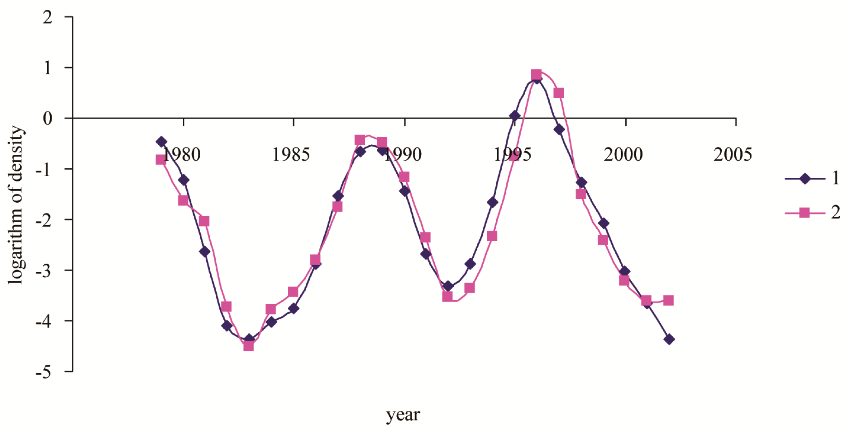
- Several time series of area S of seasonal pest damage in a small area. These time series were analyzed for such territories as the states of Massachusetts, New Hampshire, and New Jersey in the USA [13], data on area S of damaged forests in the Tyumen region (Russia) and in Japan (prefectures Hokkaido and Niigata), and data on the average level P of damage to tree crowns on test plots in the northwestern part of France (46.00–49.00° N, 0–1.00° E). Spongy moth habitat and observation points are shown in Figure 1.
2.2. Methods
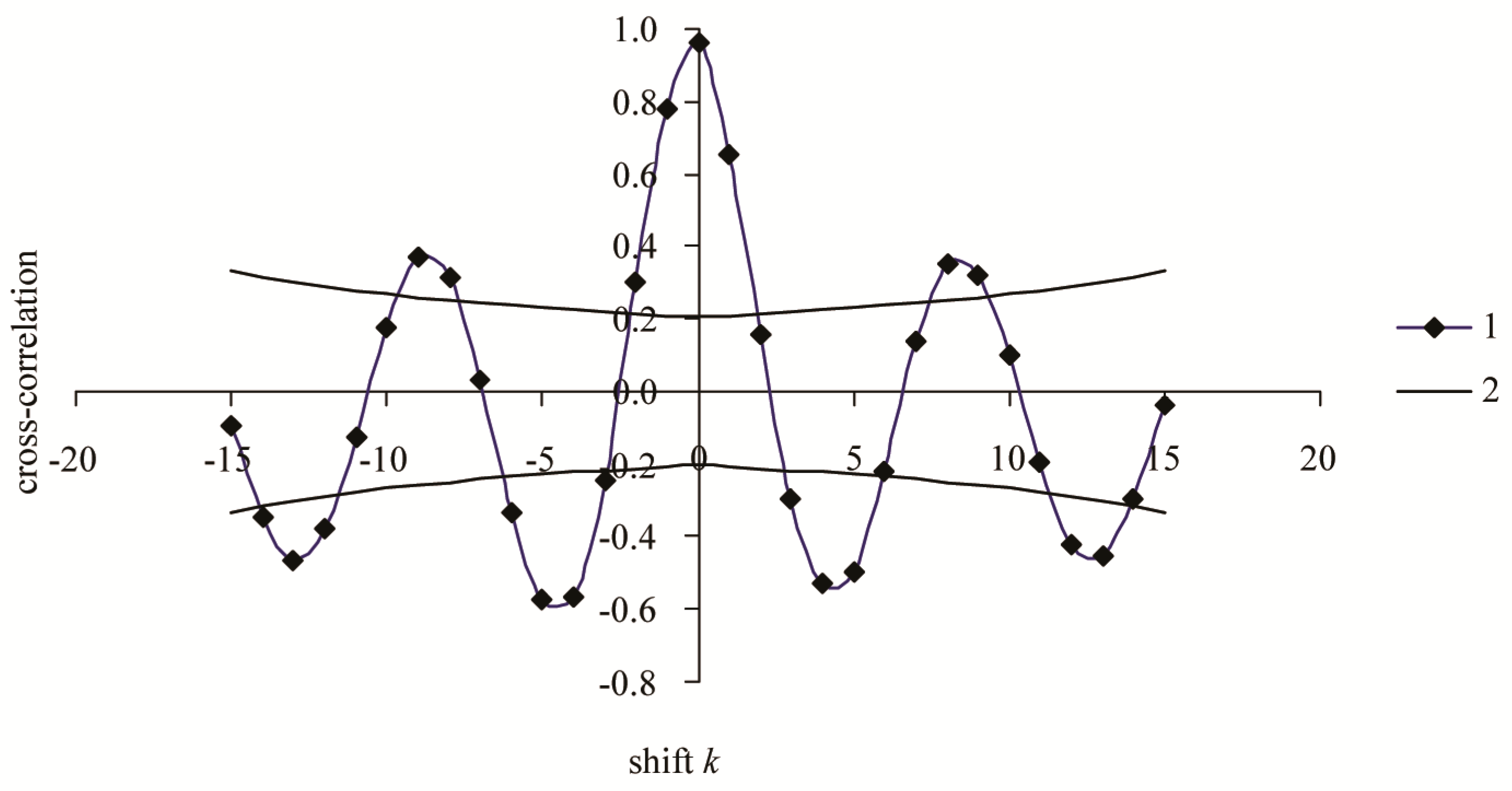
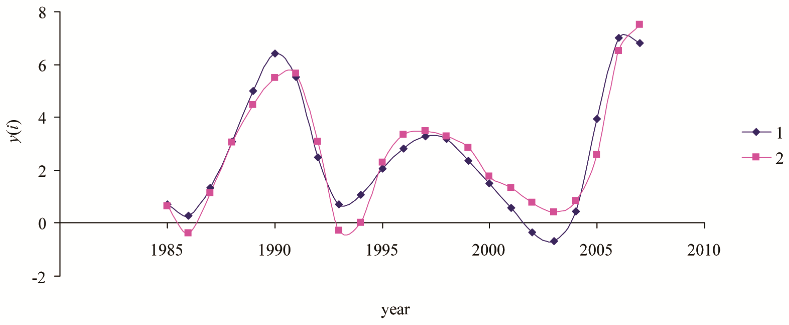
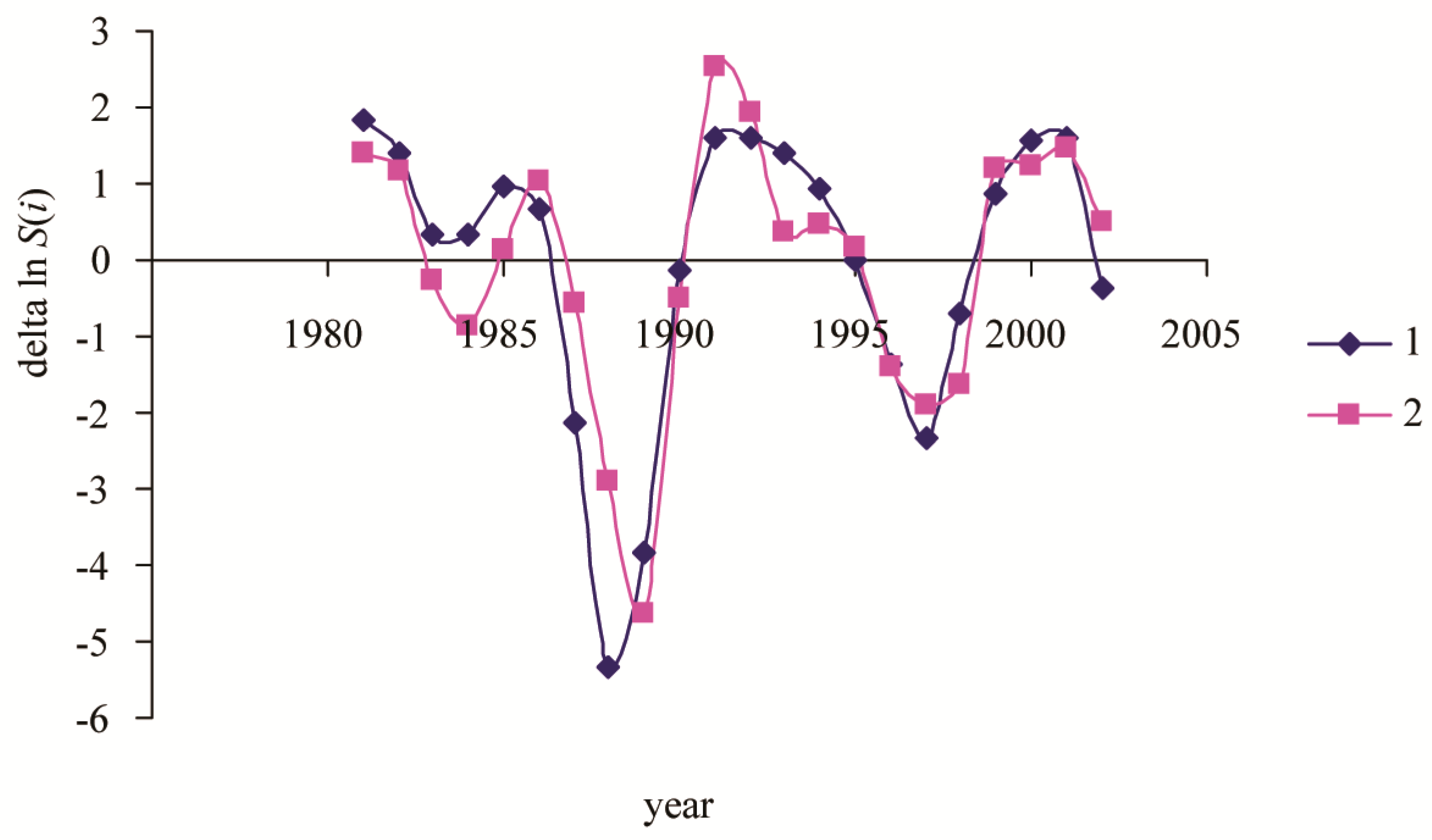
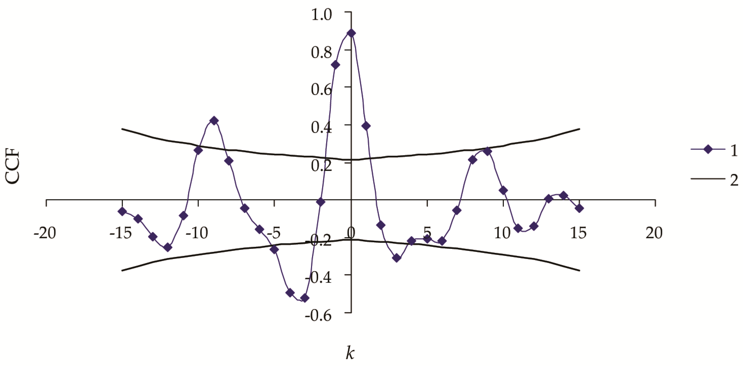
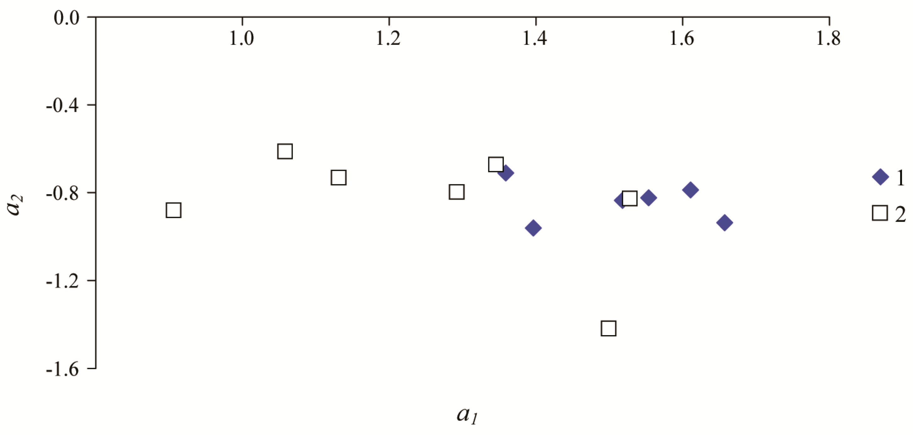
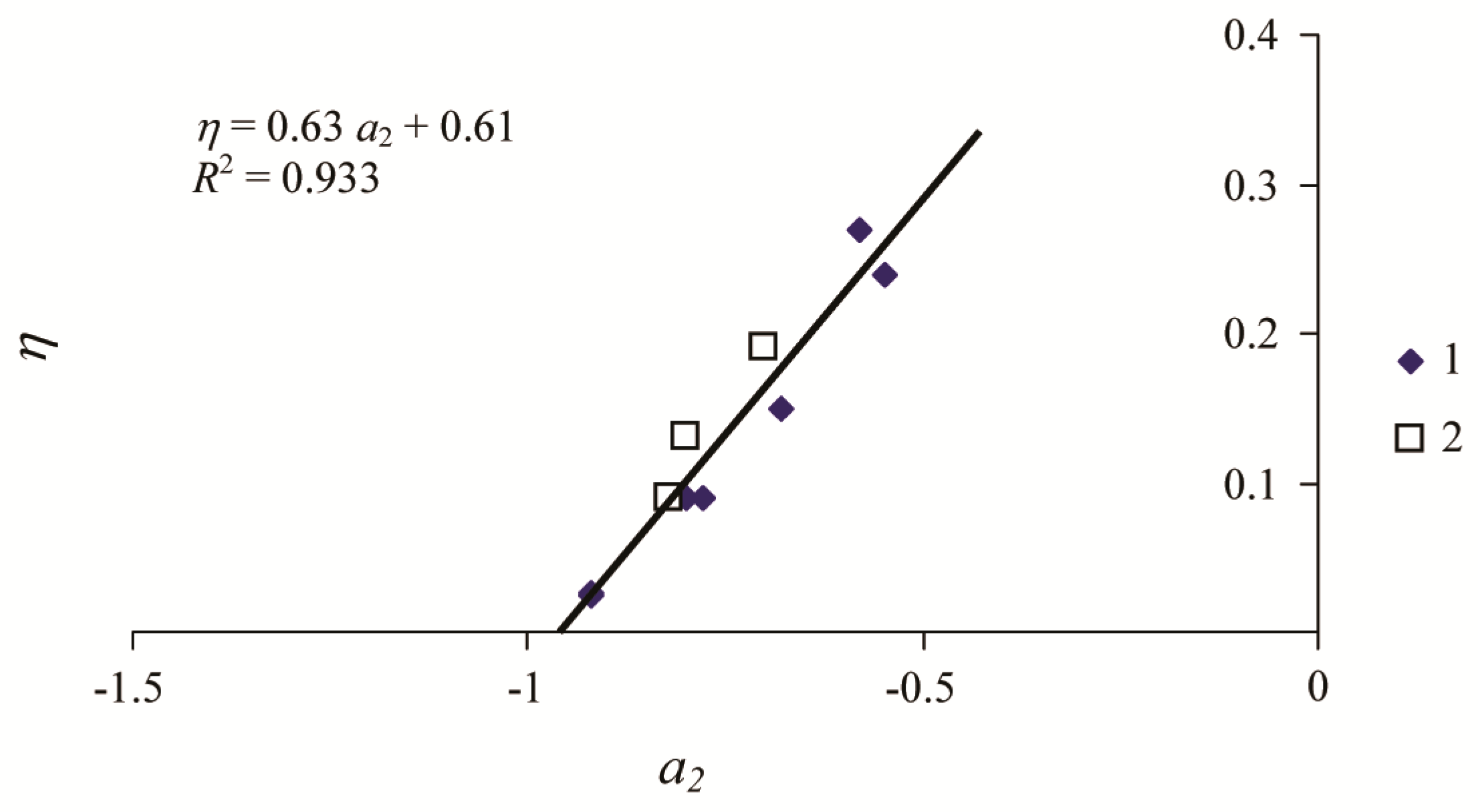
3. Results
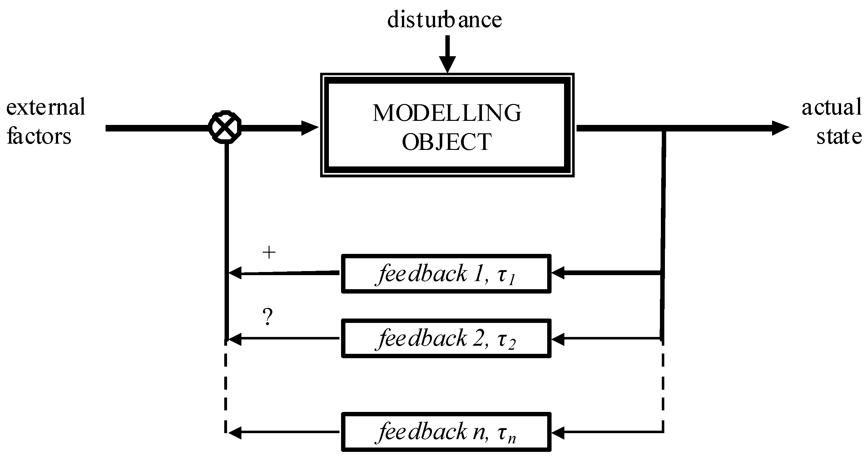
4. Discussion
- -
- Alterations of the parameters of the population and of its natural environment owing to various circumstances;
- -
- The population’s and its natural environment’s properties that are not taken into account in the model;
- -
- The lag—during an interaction of the population with its environment—is not taken into consideration in the model;
- -
- A change in the stable state of the population;
- -
- Errors in the monitoring of population size;
- -
- Unpredictable external factors.
5. Conclusions
Supplementary Materials
Author Contributions
Funding
Data Availability Statement
Conflicts of Interest
References
- Lotka, A.J. Elements of Physical Biology; Williams and Wilkins: Baltimore, MD, USA, 1925; 460p. [Google Scholar]
- Volterra, V. Leçons sur la Théorie Mathématique de la Lutte pour la Vie; Gauthier-Villars: Paris, France, 1931; 214p. (In French) [Google Scholar]
- Berryman, A.A. Population Systems: A General Introduction; Plenum Press: New York, NY, USA, 1981; 222p. [Google Scholar]
- Berryman, A.A. Dynamics of Forest Insect Populations; Plenum Press: New York, NY, USA, 1988; 603p. [Google Scholar]
- Turchin, P. Rarity of density dependence or population regulation with lags? Nature 1990, 34, 660–663. [Google Scholar] [CrossRef]
- Turchin, P. Complex Population Dynamics: A Theoretical/Empirical Synthesis; Princeton University Press: Princeton, NJ, USA, 2003; 536p. [Google Scholar]
- Soetaert, K.; Herman, P.M.J. A Practical Guide to Ecological Modelling. Using R as a Simulation Platform; Springer: Berlin/Heidelberg, Germany, 2009; 372p. [Google Scholar]
- Sharov, A.A.; Colbert, J.J. A model for testing hypotheses of gypsy moth, Lymantria dispar L., population dynamics. Ecol. Model. 1996, 84, 31–51. [Google Scholar] [CrossRef]
- Soukhovolsky, V.G.; Ponomarev, V.I.; Sokolov, G.I.; Tarasova, O.V.; Krasnoperova, P.A. Gypsy moth Lymantria dispar L. in the Southern Urals: Features of population dynamics and modeling. Russian J. Gen. Biol. 2015, 3, 179–194. (In Russian) [Google Scholar] [CrossRef]
- Inoue, M.N.; Suzuki-Ohno, Y.; Haga, Y.; Aarai, H.; Sano, T.; Martemyanov, V.; Kunimi, Y. Population dynamics and geographical distribution of the gypsy moth, Lymantria dispar, in Japan. For. Ecol. Manag. 2019, 434, 154–164. [Google Scholar] [CrossRef]
- Martemyanov, V.; Bykov, R.; Demenkova, M.; Gninenko, Y.; Romancev, S.; Bolonin, I.; Mazunin, I.; Belousova, I.; Akhanaev, Y.; Pavlushin, S.; et al. Genetic evidence of broad spreading of Lymantria dispar in the West Siberian Plain. PLoS ONE 2019, 14, e0220954. [Google Scholar] [CrossRef] [PubMed]
- Martemyanov, V.V.; Belousova, I.A.; Pavlushin, S.V.; Dubovskiy, I.M.; Ershov, N.I.; Alikina, T.Y.; Kabilov, M.R.; Glupov, V.V. Phenological asynchrony between host plant and gypsy moth reduces insect gut microbiota and susceptibility to Bacillus thuringiensis. Ecol. Evol. 2016, 6, 7298–7310. [Google Scholar] [CrossRef]
- Johnson, D.J.; Liebhold, A.M.; Bjornstad, O.N.; McManus, M.L. Circumpolar variation in periodicity and synchrony among gypsy moth populations. J. Anim. Ecol. 2005, 74, 882–892. [Google Scholar] [CrossRef]
- Allen, J.C.; Foltz, J.L.; Dixon, W.N.; Liebhold, A.M.; Colbert, J.J.; Regniere, J.; Gray, D.R.; Wilder, J.W.; Christie, I. Will the Gypsy Moth Become a Pest in Florida? Fla. Entomol. 1993, 76, 102–113. [Google Scholar] [CrossRef]
- Sharov, A.; Leonard, D.; Liebhold, A.; Roberts, E.; Dickerson, W. “Slow The Spread”: A National Program to Contain the Gypsy Moth. J. For. 2002, 100, 30–35. [Google Scholar] [CrossRef]
- Tobin, P.; Bai, B.; Eggen, D.; Leonard, D. The ecology, geopolitics, and economics of managing Lymantria dispar in the United States. Int. J. Pest Manag. 2012, 58, 195–210. [Google Scholar] [CrossRef]
- Berryman, A.A. What caused population cycles of forest Lepidoptera? Treands Ecol. Evol. 1995, 11, 28–32. [Google Scholar] [CrossRef] [PubMed]
- Bigsby, K.; Tobin, P.; Sills, E. Anthropogenic drivers of gypsy moth spread. Biol. Invasions 2011, 13, 2077–2090. [Google Scholar] [CrossRef]
- Gninenko, Y.; Orlinskii, A. Outbreaks of Lymantria dispar in Russian forests during the 1990’s. EPPO Bull. 2003, 33, 325–329. [Google Scholar] [CrossRef]
- Elkinton, J.S. Population dynamics of gypsy moth in North America. Ann. Rev. Entom. 1990, 35, 517–596. [Google Scholar] [CrossRef]
- Gray, D.R.; Logan, J.A.; Ravlin, F.W.; Carlson, J.A. Toward a model of gypsy moth egg phenology: Using respiration rates of individual eggs to determine temperature-time requirements of pre-diapause development. Environ. Entomol. 1991, 20, 1645–1652. [Google Scholar] [CrossRef]
- Johnson, D.M.; Liebhold, A.M.; Tobin, P.C.; Bjornstad, O.N. Allee effects and pulsed invasion by the gypsy moth. Nature 2006, 444, 361–363. [Google Scholar] [CrossRef] [PubMed]
- Keena, M.A. Comparision of the hatch of Limantria dispar (Lepidoptera: Lymantriidae) eggs from Russia and the United States after exposure to different temperatures and duration of low temperature. Ann. Entomol. Soc. Am. 1996, 89, 564–572. [Google Scholar] [CrossRef]
- Williams, D.W.; Liebhold, A.M. Influence of weather on the synchrony of gypsy moth (Lepidoptera: Lymantriidae) outbreaks in New England. Environ. Entomol. 1995, 24, 987–995. [Google Scholar] [CrossRef]
- Liebhold, A.M. Are North American populations of gypsy moth (Lepidoptera: Lymantriidae) bimodal? Environ. Entomol. 1992, 21, 221–229. [Google Scholar] [CrossRef]
- Wilder, J.W.; Voorhis, N.; Colbert, J.J.; Sharov, A.A. Three variable differential equation model for gypsy moth population dynamics. Ecol. Model. 1994, 72, 229–250. [Google Scholar] [CrossRef]
- Williams, D.W.; Fuester, R.W.; Metterhouse, W.W.; Balaam, R.J.; Bullock, R.H.; Chianese, R.I.; Reardon, R.C. Density, size and mortality of egg masses in New Jersey of the gypsy moth (Lepidoptcra: Lymantriidae). Environ. Entomol. 1990, 19, 943–948. [Google Scholar] [CrossRef]
- Lyamtsev, N.I. Prediction of the Gypsy Moth Outbreaks, the Threat of Damage to Oak Forests and the Need for Protective Measures; VNILM: Puschino, Russia, 2018; 84p. (In Russian) [Google Scholar]
- Benkevich, V.I. Mass Appearances of the Gypsy Moth in the European Part of the USSR. Nauka: Moscow, Russia, 1984; 143p. (In Russian) [Google Scholar]
- Jurchenko, G.N.; Turova, G.N. Population dynamics of the Asian gypsy moth in the Far Eastern part of the range. For. Messenger 2009, 5, 97–109. [Google Scholar]
- Cobb, C.W.; Douglas, P.H. A Theory of Production. Am. Econ. Rev. 1928, 18, 139–165. [Google Scholar]
- Nechyba, T.J. Microeconomics: An Intuitive Approach with Calculus; Cengage Learning: Boston, MA, USA, 2011; 1206p. [Google Scholar]
- Jacques, I. Mathematics for Economics and Business, 9th ed.; Pearson Education: Harlow, UK, 2018; 752p. [Google Scholar]
- Stock, J.H.; Watson, W. Introduction to Econometrics; Addison Wesley: Boston, MA, USA, 2007; 840p. [Google Scholar]
- Isaev, A.S.; Soukhovolsky, V.G.; Tarasova, O.V.; Palnikova, E.N.; Kovalev, A.V. Forest Insect Population Dynamics, Outbreaks and Global Warming Effects; Wiley: New York, NY, USA, 2017; 298p. [Google Scholar]
- Jenkins, G.M.; Watts, D.G. Spectral Analysis and Its Applications; Holden-Day: San Francisco, CA, USA, 1969; 525p. [Google Scholar]
- Royama, T. Analytical Population Dynamics; Chapman and Hall: Boca Raton, FL, USA, 1992; 371p. [Google Scholar]
- Dorf, R.C.; Bishop, R.H. Modern Control Systems; Prentice Hall: Hoboken, NJ, USA, 2008; 1018p. [Google Scholar]
- Barker, K.L. Mikhailov Stability Criterion for Time-Delayed Systems; NASA Technical Memorandum 78803 Langley Research Center National Aeronautics and Space Administration: Hampton, VA, USA, 1978; 28p.
- Gopalsamy, K. Stability and Oscillations in Delay Differential Equations of Population Dynamics; Kluwer Academic Publishers: Dordrecht, The Netherlands, 1992; 501p. [Google Scholar]
- Stanisławski, R. Modified Mikhailov stability criterion for continuous-time noncommensurate fractional-order systems. J. Frankl. Inst. 2022, 359, 1677–1688. [Google Scholar] [CrossRef]
- Hamming, R.W. Digital Filters; Courier Corporation: North Chelmsford, MA, USA, 1989; 284p. [Google Scholar]
- Anderson, T.W. The Statistical Analysis of Time Series; John Wiley & Sons, Inc.: Hoboken, NJ, USA, 1971; 704p. [Google Scholar]
- Pollard, J.H. A Handbook of Numerical and Statistical Techniques; Cambridge University Press: Cambridge, UK, 1979; 368p. [Google Scholar]
- Soukhovolsky, V.; Kovalev, A.; Tarasova, O.; Modlinger, R.; Krenová, Z.; Mezei, P.; Škvarenina, J.; Rožnovský, J.; Korolyova, N.; Majdák, A.; et al. Wind Damage and Temperature Effect on Tree Mortality Caused by Ips typographus L.: Phase Transition Model. Forests 2022, 13, 180. [Google Scholar] [CrossRef]
- Isaev, A.S.; Rozhkov, A.S.; Kiselev, V.V. Black Fir Sawyer Beetle; Nauka: Novosibirsk, Russia, 1988; 270p. (In Russian) [Google Scholar]
- Mori, N.; Kawatsu, K.; Noriyuki, S.; Kosilov, A.; Martemyanov, V.; Yamashita, M.; Inoue, M.N. Monitoring and prediction of the spongy moth (Lymantria dispar) outbreaks in Mountain’s landscape using a combination of Sentinel-2 images and nonlinear time series model. For. Ecol. Manag. 2024, 563, 121975. [Google Scholar] [CrossRef]


| Variables/Parameters | Value | Std.Err. | t(20) Test | p-Value |
|---|---|---|---|---|
| ln HTC(i, 4)/b | −0.248 | 0.185 | −1.342 | 0.1948 |
| y(i − 2)/a2 | −0.822 | 0.106 | −7.730 | 0.0000 |
| y(i − 1)/a1 | 1.553 | 0.110 | 14.111 | 0.0000 |
| Radj2 | 0.91 | |||
| F test | 78.4 | |||
| η | 0.09 | |||
| Variables | Value | Std.Err. | t Test | p-Value |
|---|---|---|---|---|
| Moscow region, eggs, 1951–1964. | ||||
| ln HTC(i, 4) | −0.125 | 0.040 | 3.125 | 0.013 |
| y(i − 2) | −0.939 | 0.093 | −10.139 | 0.000 |
| y(i − 1) | 1.657 | 0.102 | 16.231 | 0.000 |
| Radj2 | 0.97 | |||
| F test | 156.00 | |||
| η | 0.03 | |||
| Chelyabinsk region, forest-steppe zone, eggs, 1960–2010 | ||||
| ln HTC(i, 4) | −0.200 | 0.163 | −1.223 | 0.228 |
| y(i − 2) | −0.708 | 0.100 | −7.065 | 0.000000 |
| y(i − 1) | 1.359 | 0.100 | 13.555 | 0.000000 |
| Radj2 | 0.815 | |||
| F test | 71.50 | |||
| η | 0.17 | |||
| Chelyabinsk region, steppe zone, eggs, 1960–2010 | ||||
| HTC(i, 4) | −0.073 | 0.033 | −2.210 | 0.036 |
| y(i − 2) | −0.790 | 0.134 | −5.880 | 0.000003 |
| y(i − 1) | 1.610 | 0.130 | 12.374 | 0.000000 |
| Radj2 | 0.916 | |||
| F test | 109.70 | |||
| η | 0.09 | |||
| Khabarovsk region, eggs, 1984–2008 | ||||
| ln HTC(i, 5) | −0.082 | 0.246 | −0.334 | 0.742 |
| y(i − 2) | −0.937 | 0.107 | −8.775 | 0.000000 |
| y(i − 1) | 1.389 | 0.097 | 14.267 | 0.000000 |
| Radj2 | 0.91 | |||
| F test | 67.9 | |||
| η | 0.04 | |||
| Variables | Value | Std.Err. | t Test | p-Value |
|---|---|---|---|---|
| ln HTC(i, 4) | −0.669 | 0.538 | −1.242 | 0.230 |
| DSS(i − 2) | −0.734 | 0.153 | −4.795 | 0.000145 |
| DSS(i − 1) | 1.131 | 0.147 | 7.696 | 0.000000 |
| Radj2 | 0.79 | |||
| F test | 21.9 | |||
| η | 0.20 | |||
| Variables | Value | Std.Err. | t Test | p-Value |
|---|---|---|---|---|
| Massachusetts (USA), 1979–2002 | ||||
| ln HTC(i, 4) | −0.669 | 0.538 | −1.242 | 0.230 |
| DSS(i − 2) | −0.734 | 0.153 | −4.795 | 0.000145 |
| DSS(i − 1) | 1.131 | 0.147 | 7.696 | 0.000000 |
| Radj2 | 0.79 | |||
| F test | 21.9 | |||
| η | 0.20 | |||
| New Hampshire (USA), 1979–2002 | ||||
| ln HTC(i, 4) | −1.291 | 0.741 | −1.743 | 0.10058 |
| DSS(i − 2) | −0.833 | 0.104 | −7.980 | 0.000001 |
| DSS(i − 1) | 1.528 | 0.108 | 14.156 | 0.000000 |
| Radj2 | 0.92 | |||
| F test | 75.3 | |||
| η | 0.09 | |||
| New Jersey (USA), 1979–2002 | ||||
| ln HTC(i, 4) | −0.204 | 0.324 | −0.629 | 0.538 |
| DSS(i − 3) | 0.609 | 0.264 | 2.303 | 0.035 |
| DSS(i − 2) | −1.423 | 0.273 | −5.217 | 0.000085 |
| DSS(i − 1) | 1.500 | 0.236 | 6.363 | 0.000009 |
| Radj2 | 0.78 | |||
| F test | 18.42 | |||
| η | 0.33 | |||
| Western France (46.0–49.0° N, 0–1.0° E) (2008–2020) | ||||
| ln T(i, 4) | 0.098 | 2.104 | 0.047 | 0.964 |
| ln P(i − 2) | −0.830 | 0.315 | −2.637 | 0.0336 |
| ln P(i − 1) | 1.012 | 0.277 | 3.655 | 0.0081 |
| Radj2 | 0.60 | |||
| F test | 6.09 | |||
| η | 0.14 | |||
| Tyumen region (Russia) | ||||
| ln HTC(i, 5) | −0.942 | 0.450 | −2.093 | 0.053 |
| ln S(i − 2) | −0.594 | 0.189 | −3.147 | 0.0062 |
| ln S(i − 1) | 1.251 | 0.178 | 7.036 | 0.000003 |
| Radj2 | 0.81 | |||
| F test | 27.8 | |||
| η | 0.24 | |||
| Hokkaido (Japan), 1979–2009 | ||||
| ln HTC(i, 5) | −0.057 | 0.143 | 1.070 | 0.07 |
| ln S(i − 2) | −0.610 | 0.156 | −3.941 | 0.00052 |
| ln S(i − 1) | 1.046 | 0.156 | 6.804 | 0.000000 |
| Radj2 | 0.64 | |||
| F test | 15.8 | |||
| η | 0.29 | |||
| Niigata (Japan), 1961–1974 | ||||
| ln T(i, 4) | 0.164 | 0.083 | 1.990 | 0.086 |
| y(i − 2) | −0.967 | 0.178 | −5.434 | 0.00097 |
| y(i − 1) | 0.187 | 0.251 | 0.747 | 0.479 |
| Radj2 | 0.78 | |||
| F test | 12.80 | |||
| η | 0.033 | |||
| Habitat | Massachusetts (USA) | New Jersey (USA) | New Hampshire (USA) | Tour (France) |
| Month | April | April | May | April |
| Average air temperature, °C | 7.80 | 9.12 | 12.03 | 11.58 |
| Standard error | 0.22 | 0.23 | 0.24 | 0.41 |
| Habitat | Saratov Region (Russia) | Tyumen Region (Russia) | Niigata (Japan) | Hokkaido (Japan) |
| month | April | May | April | May |
| Average air temperature, °C | 8.43 | 11.84 | 10.83 | 10.07 |
| Standard error | 0.37 | 0.36 | 0.25 | 0.15 |
Disclaimer/Publisher’s Note: The statements, opinions and data contained in all publications are solely those of the individual author(s) and contributor(s) and not of MDPI and/or the editor(s). MDPI and/or the editor(s) disclaim responsibility for any injury to people or property resulting from any ideas, methods, instructions or products referred to in the content. |
© 2024 by the authors. Licensee MDPI, Basel, Switzerland. This article is an open access article distributed under the terms and conditions of the Creative Commons Attribution (CC BY) license (https://creativecommons.org/licenses/by/4.0/).
Share and Cite
Soukhovolsky, V.; Kovalev, A.; Akhanaev, Y.; Kurenshchikov, D.; Ponomarev, V.; Tarasova, O.; Caroulle, F.; Inoue, M.N.; Martemyanov, V. An Autoregulatory Model of Forest Insect Population Dynamics and Forest Stand Damage Dynamics in Different Habitats: An Example of Lymantria dispar L. Forests 2024, 15, 1098. https://doi.org/10.3390/f15071098
Soukhovolsky V, Kovalev A, Akhanaev Y, Kurenshchikov D, Ponomarev V, Tarasova O, Caroulle F, Inoue MN, Martemyanov V. An Autoregulatory Model of Forest Insect Population Dynamics and Forest Stand Damage Dynamics in Different Habitats: An Example of Lymantria dispar L. Forests. 2024; 15(7):1098. https://doi.org/10.3390/f15071098
Chicago/Turabian StyleSoukhovolsky, Vladislav, Anton Kovalev, Yuriy Akhanaev, Dmitry Kurenshchikov, Vasiliy Ponomarev, Olga Tarasova, Fabien Caroulle, Maki N. Inoue, and Vyacheslav Martemyanov. 2024. "An Autoregulatory Model of Forest Insect Population Dynamics and Forest Stand Damage Dynamics in Different Habitats: An Example of Lymantria dispar L." Forests 15, no. 7: 1098. https://doi.org/10.3390/f15071098