Functional Traits Affect the Contribution of Individual Species to Beta Diversity in the Tropical Karst Seasonal Rainforest of South China

Abstract

In a community, due to the different characteristics of each species, their contributions to community beta diversity may vary. Quantifying the contribution of each species to overall beta diversity (SCBD) is essential for explaining the patterns of beta diversity. However, there is currently limited research linking SCBD with species functional traits, and how species functional traits influence SCBD remains unclear. This study is based on tree census data, species functional traits, and environmental variables from a 15 ha permanent monitoring plot in a tropical karst rainforest in south China. By calculating species-specific SCBD based on abundance and presence–absence data, as well as functional distinctiveness and species ecological niche characteristics (niche position and niche width), we applied structural equation modeling (SEM) to analyze how functional traits, distinctiveness, and niche characteristics jointly influence SCBD. The results revealed that SCBD based on abundance is positively correlated with occupancy and abundance, whereas SCBD based on presence–absence data exhibits a hump-shaped relationship with occupancy and abundance. Species ecological niche characteristics directly influence SCBD, with species occupying central ecological niches having a negative effect on SCBD and niche width having a positive effect. Functional traits and functional distinctiveness indirectly impact SCBD through their influence on species ecological niche characteristics. SEM models based on the presence–absence data provide higher explanatory power. In summary, in the seasonal rainforest communities of northern tropical karst regions in China, the combined effects of species’ functional traits, functional distinctiveness, and ecological niche characteristics determine SCBD. This not only contributes to a deeper understanding of how species traits influence β-diversity, making SCBD a more applicable tool for biodiversity conservation, but also allows for the development of more effective biodiversity protection strategies by elucidating the link between SCBD and ecosystem multifunctionality.

1. Introduction

The distribution pattern of biodiversity is closely related to the research scale, and the variation pattern of biodiversity along environmental gradients is an important topic in ecological research [1]. According to Whittaker’s [2] perspective, biodiversity can be categorized into three main hierarchical levels: α-diversity, β-diversity, and γ-diversity. Among these, α-diversity primarily focuses on the number of species in local homogeneous habitats. γ-diversity describes diversity at the regional or continental scale. Meanwhile, β-diversity represents the variation in species composition between locations and serves as an important indicator of community structure. It is related to the allocation of environmental resources among species and is widely understood in the field of ecology as the differences in species composition between different locations [3,4]. Since its conceptualization, β-diversity has become a key factor for better understanding the origin, function, and maintenance of biodiversity [5]. To estimate β-diversity, various indices and methods have been proposed, including presence–absence or abundance data, multiplicative indices, and additive partitioning of community diversity [6]. For instance, Legendre and Cáceres [3] proposed a method that involves calculating the total β-diversity (BD_total) using a community composition matrix (site × species); this approach allows for assessing the contribution of individual species to BD_total (referred to as SCBD) within specific communities. By exploring patterns of β-diversity, we gain important insights into the mechanisms behind the community structuring and biodiversity maintenance, which may be used for biodiversity conservation and ecological restoration [7].

In ecology, β-diversity is typically assessed through two dimensions: local contributions to beta diversity (LCBD), which represents the contribution of individual sites to overall β-diversity; and species contributions to beta diversity (SCBD), which measures the contribution of each species to differences in species composition between different communities. LCBD reflects the uniqueness of each location within the overall β-diversity and is associated with various environmental and spatial variables, while SCBD quantifies the role of each species in the variation in species composition across different communities [8,9]. In recent years, research on SCBD and LCBD has gradually increased. Da Silva et al. [10] investigated the correlation between species and site contributions to β-diversity in beetle communities, they found that both SCBD and LCBD are highly predictable based on species occupancy and species richness. Krasnov et al. [11] investigated the contributions of species and sites to β-diversity in parasitic fleas of small mammals in the Greater Khingan Mountains, they found that the SCBD of fleas can be predicted based on their ecological and geographical characteristics, while the combined LCBD can be predicted based on host composition. Compared to the attention given to LCBD, the ecological relevance of SCBD has received relatively less focus [10,12], primarily emphasizing animal taxonomic groups [5,10].

SCBD is related to general species characteristics, such as occupancy, abundance, niche location, niche width, and species biology [8]. The study found that there was a significant positive correlation between species abundance, occupancy, and SCBD, but there was no significant correlation between SCBD and niche breadth [8,12]. Da Silva et al. [10] observed that SCBD is related to the ecological niche position of beetles, but not to the ecological niche width. Functional traits can predict species–environment interactions, thereby explaining patterns of species abundance and occupancy in a community, and therefore, functional traits should influence SCBD [9]. There are also studies that find that SCBD is not correlated or weakly correlated with species biological traits [8,10], which may only consider the direct effects of traits and ignore the indirect effects. However, there are still many difficulties and challenges in the study of β-diversity, and more in-depth exploration is needed to understand the complex relationship between species characteristics and SCBD.

In order to effectively link community structure with ecosystem function, the role of functional traits should be considered [9,13]. In terms of species functional trait combinations, the Functional Distinctiveness Index quantifies the degree to which a combination of traits for a single species is uncommon on a local scale [14]. At the local scale, functional distinctiveness considers all species within a community to measure whether an individual species is becoming functionally more similar to other species in the community. Since species functional distinctiveness is relative to a given combination, the value of functional distinctiveness largely depends on the spatial scale defining that combination [15,16]. Gaüzère et al. [16] found significant differences in functional distinctiveness of many species (particularly between regional and community scales), with a general trend of lower distinctiveness at smaller scales. In addition, species with high functional distinctiveness may have unique niche attributes that are different from other species in terms of resource use, environmental adaptation, or survival strategies [17]. Moreover, more unique combinations of traits may result from specific habitat survival strategies that species adopt to avoid competition with other species, this implies that the survival range of species is narrower, and their ecological niche breadth is smaller [18]. Functional distinctiveness is associated with species ecological niche characteristics, thereby influencing species abundance and occupancy. Therefore, functional distinctiveness may impact species SCBD. Revealing how functional distinctiveness influences SCBD aids in a profound understanding of beta diversity patterns at a local scale, shedding light on how different species coexist within the same habitat and their roles within the ecosystem.

In karst ecosystems, due to the large-scale exposure of bedrock and the long-term dual effects of dissolution and weathering, a variety of complex and intertwined microenvironmental structures have been formed on the surface, including karst ditches, rock crevices, stone ridges, and exposed rocks [19,20]. The northern tropical karst seasonal rainforest is one of the typical forest vegetation types distributed in the karst regions of the northern tropical edge of China. It is also one of the global biodiversity hotspots [21]. The forest in this region exhibits diverse community structures, rich species composition, and prominent endemic components [22]. As a typical representative of karst forest, this kind of rainforest is an important reference system for vegetation management and reconstruction in karst areas [23]. In recent years, research on the northern tropical karst seasonal rainforest has mainly focused on aspects such as species composition, spatial distribution, and species diversity [24,25]. However, there have been no reports on how plant functional traits in karst regions influence the contributions of individual species to β-diversity.

Currently, despite Wang et al. [9] having explored the joint effects of functional distinctiveness and ecological niche properties on SCBD in subtropical forests of southern China using functional trait features and environmental variables, research linking plant functional traits to SCBD remains limited. Particularly, relevant studies in karst regions are still lacking. Therefore, this study aims to extend Wang et al.’s work. In addition to analyzing the relationship between SCBD and occupancy and abundance based on abundance data and presence–absence data, we further investigate how functional distinctiveness, ecological niche position, and ecological niche breadth collectively influence SCBD in a northern tropical karst seasonal rainforest. In this way, we aim to reveal the mechanistic relationships between plant functional traits, functional distinctiveness, ecological niche position, ecological niche breadth, and SCBD, and assess the importance of these features in this ecosystem.

The Nonggang northern tropical karst seasonal rainforest exhibits globally representative characteristics of tropical karst forests, with diverse microhabitats and complex community structures [22]. This study is based on a 15 ha permanent monitoring plot in the Nonggang karst seasonal rainforest. Using data from species inventories within the plot, species functional traits, and environmental variables, we calculated species-level SCBD (species co-occurrence-based diversity), functional distinctiveness, and ecological niche characteristics. We also employed structural equation modeling (SEM) to explore whether functional traits, functional distinctiveness, and niche characteristics (position and breadth) influence SCBD [26]. We aimed to answer the following scientific questions: (a) How do niche characteristics of species affect SCBD? (b) How do functional traits and functional distinctiveness influence SCBD? (c) What is the relative contribution of various variables to SCBD?

2. Materials and Methods

2.1. Study Area

The Guangxi Nonggang National Nature Reserve (NNNR) is located at the junction of Longzhou County and Ningming County in Chongzuo City, Guangxi, China (106.71°–107.08° E, 22.23°–22.55° N). It extends in a southeast to northwest direction and covers an area of approximately 10,077.5 hectares, with elevations ranging from 300 to 600 m. The reserve experiences a tropical monsoon climate, with an average annual temperature of 22 °C. The highest temperatures can reach 37–39 °C, and there are 7 months with average monthly temperatures exceeding 22 °C. The coldest month has an average temperature higher than 13 °C. Additionally, the annual average rainfall ranges from 1150 to 1550 mm, concentrated mainly from May to September. The maximum recorded rainfall reached 2043 mm, while the minimum was 890 mm [25].

The study area is a 15-hectare forest dynamics monitoring plot located within the NNNR. The plot was established in 2011, and its construction followed the protocols by the Center for Tropical Forest Science (CTFS) [23]. The study site is located in the core area of the NNNR, with geographical coordinates at 22.25° N and 106°57′ E. The site extends 300 m north–south and 500 m east–west, with an elevation ranging from 180 to 370 m. The forest type belongs to the north tropical karst seasonal rainforest. In 2011, the first community survey was conducted within this site. All woody plants with a diameter at breast height (DBH) greater than or equal to 1 cm were identified, and their species names, DBH measurements, and coordinates were recorded. These plants were marked and monitored over the long term. The most recent census, completed in 2021, revealed a total of 74,925 independent trees and shrubs belonging to 207 species within the survey area. Prior to modeling, the entire 15-hectare site was divided into 375 quadrats of 20 m × 20 m.

2.2. Sampling Methods

2.2.1. Functional Traits

This study selected six functional traits, including the leaf traits specific leaf area (SLA), leaf dry matter content (LDMC), leaf carbon content (LC), leaf nitrogen content (LN), and leaf phosphorus content (LP); and the stem trait wood density (WD) [27]. The process of obtaining functional trait data is as follows: First, for all surveyed tree species within the plot, branches and leaves were collected and measured. The specific method involved randomly selecting small branches from the outer canopy layer of each tree, ensuring that there was no significant leaf area loss. From these small branches, fully expanded intact leaves were chosen, and they were cut into approximately 10 cm long segments using pruning shears. These segments were placed in self-sealing bags, and their species and identification numbers were recorded on the bags. Back indoors, the fresh leaf weight (FLW), leaf area (LA), and branch volume (BV) of the collected leaves and branches were measured. Next, the collected leaves and branches were dried at a constant temperature of 60 °C until they reached a constant weight, and then, the leaf dry weight (LDW) and branch dry matter (BDM) content were measured. Here are the formulas for calculating specific leaf area (SLA), leaf dry matter content (LDMC), and wood density (WD) using the provided data [28]:

$$SLA=\frac{LA}{LDW}$$

(1)

$$LDMC=\frac{LDW}{FLW}$$

(2)

$$WD=\frac{BDM}{BV}$$

(3)

In addition, the leaves dried to a constant weight were crushed for elemental analysis. Elemental analysis was used to determine leaf carbon content, the Kjeldahl method was used to measure leaf nitrogen content, and the molybdate colorimetric method was employed to assess leaf phosphorus content [28].

2.2.2. Environmental Data

The environmental data include topographic factors, average elevation, slope, and converted aspect; and soil factors, moisture content, bulk density, total nitrogen, total carbon, total phosphorus, total potassium, organic matter, calcium, magnesium, and pH. Topographic data were collected at the quadrat level (20 m × 20 m) by recording elevation, aspect, and slope for each quadrat. The conversion of aspect direction was based on a method used by previous researchers [29], which transformed compass measurements from the 0–360° range to a 0–1 scale. The conversion formula is as follows:

$$TRASP=\frac{(\mathsf{\pi }÷180)(\mathrm{a}\mathrm{s}\mathrm{p}\mathrm{e}\mathrm{c}\mathrm{t}-30)}{2}$$

(4)

Among these, TRASP represents the aspect index, where aspect denotes the angle of the slope direction. After conversion, the TRASP values range from 0 to 1. A higher TRASP value indicates a drier and hotter habitat. Specifically, 0 corresponds to the north–northeast direction, while 1 corresponds to the south–southwest direction.

The soil data were collected using soil augers from 375 quadrats of 20 m × 20 m at the surface layer (0–20 cm) and placed in soil collection bags. After bringing the soil samples back to the laboratory, impurities were removed, and the samples were naturally air-dried, ground, and sieved for chemical analysis. When conducting physicochemical analysis of soil [27,30], first, the soil samples were fused with NaOH to decompose insoluble silicates. Then, the resulting melt was dissolved in water and dilute sulfuric acid. Total phosphorus content was determined using the molybdenum antimony colorimetric method. For potassium content, the samples were acid-digested and analyzed by flame photometry. Calcium and magnesium were determined by pre-treating the soil samples with HNO₃ to remove carbonates or organic matter. Subsequently, the samples were digested with H₂SO₄-HF to break down silicates, followed by dissolution in HNO₃-H₂SO₄-HClO₄ to obtain quantifiable filtrate. Calcium and magnesium levels were measured using atomic absorption spectroscopy. Organic carbon content was determined by oxidizing soil organic matter in test tubes placed in a 180 °C oil bath for 5 min, followed by titration with a potassium dichromate–sulfuric acid solution. Soil pH was measured using a potentiometric method, while water content and bulk density were determined through drying methods. Total nitrogen and carbon content were analyzed using an elemental analyzer.

2.3. Explanatory Variables

2.3.1. Species Niche Properties

The outlying mean index (OMI) analysis was based on the above environmental factors and tree abundance data to indicate each plant species’ niche position and niche breadth [8]. In this study, two indices were selected: OMI and Tol. Specifically, OMI represents ecological niche position, measuring where a species occurs within its habitat. When most individuals of a species are found at the extreme end of an environmental gradient, the species has a higher OMI value, indicating it occupies an edge ecological niche. On the other hand, Tol represents ecological niche breadth, describing a species’ adaptation range to environmental conditions or its diversity in resource utilization. A higher Tol value indicates a wider ecological niche for the species [9,14]. These two indices reflect the interactions between species and the environment and should be related to SCBD [8,10]. The OMI is an index used to measure the distance between the average habitat conditions of a species and the sampling area. It achieves this by calculating the distance between the center of the species (representing the average habitat conditions used by the species) and the average habitat conditions of the sampling area. Specifically, before calculating the ecological niche attributes of a species, all environmental data are standardized to z-scores [31]. The calculation for the average position of species j on u (or the centroid of species j) is as follows:

$$T_j=f^{T}zu{f}^T=\left(f_{\raisebox{1ex}{$1$}\!\left/ \!\raisebox{-1ex}{$j$}\right.},\dots f_{\raisebox{1ex}{$i$}\!\left/ \!\raisebox{-1ex}{$j$}\right.},\dots f_{\raisebox{1ex}{$n$}\!\left/ \!\raisebox{-1ex}{$j$}\right.}\right)$$

(5)

$T_j$ is the OMI value of species j, z represents the standardized environmental data set, u is the normalized vector ($\left|u\right|=1$), and f denotes the frequency of species j.

Niche width is a measure of species related to environmental variables, indicating the range of distribution of species on environmental variables. It can be determined by calculating the projection of the species on the niche axis [31]. The specific calculation formula is as follows:

$$T_m\left(j\right)=\sum _{i=1}^n{f}_{\raisebox{1ex}{$i$}\!\left/ \!\raisebox{-1ex}{$j$}\right.}{‖G_j-m_i‖}^2$$

(6)

where $m_i$ represents the projection of sampling unit i on the niche axis, and $G_{ij}$ is the centroid of species j. Our study uses the “niche” function and the “niche. param” function from the “ade4” package in the R 4.3.3 software to calculate OMI and Tol values [32,33]. The OMI values and Tol values for each species can be found in the (

Table 1. Ecological niche position (OMI), ecological niche width (Tol), SCBD, and abundance of species in the 15 ha permanent monitoring plot at Nonggang.

Family	Genus	Species	OMI	Tol	SCBD	Abundance	Occupancy
Magnoliaceae	Lirianthe	fistulosa	2.7737	5.7028	0.0034	154	46
Annonaceae	Alphonsea	mollis	2.0966	2.5104	0.0016	68	49
Annonaceae	Alphonsea	monogyna	0.4583	3.5079	0.0077	504	169
Annonaceae	Desmos	chinensis	1.5410	1.3923	0.0025	126	48
Annonaceae	Goniothalamus	donnaiensis	8.5599	3.3864	0.0017	71	29
Annonaceae	Miliusa	balansae	4.9616	0.7396	0.0003	20	10
Annonaceae	Mitrephora	macclurei	7.9938	21.3198	0.0003	13	4
Annonaceae	Orophea	polycarpa	0.7544	1.7086	0.0323	2336	167
Lauraceae	Cinnamomum	saxatile	1.3120	3.5064	0.0013	63	35
Lauraceae	Cryptocarya	lyoniifolia	4.7864	3.2563	0.0047	231	94
Lauraceae	Litsea	foveola	1.2293	1.6186	0.0040	283	123
Lauraceae	Litsea	glutinosa	3.6175	0.2567	0.0001	4	4
Lauraceae	Litsea	variabilis	3.1188	2.0604	0.0013	50	20
Lauraceae	Neolitsea	hainanensis	3.3917	0.5653	0.0001	4	3
Lauraceae	Phoebe	calcarea	0.6926	0.8499	0.0006	25	16
Capparaceae	Capparis	subsessilis	19.4964	1.1943	0.0002	4	2
Capparaceae	Capparis	urophylla	0.6876	0.5002	0.0010	51	34
Violaceae	Rinorea	bengalensis	0.5558	0.6363	0.0411	2769	98
Linaceae	Tirpitzia	ovoidea	21.3642	1.2255	0.0078	514	33
Lythraceae	Lagerstroemia	caudata	2.3910	5.7955	0.0017	78	45
Pittosporaceae	Pittosporum	pulchrum	20.3276	1.7033	0.0041	269	23
Salicaceae	Bennettiodendron	leprosipes	9.3751	2.9852	0.0098	424	68
Achariaceae	Hydnocarpus	hainanensis	0.1843	1.2017	0.0216	2551	292
Salicaceae	Xylosma	longifolia	2.2536	3.3728	0.0007	31	21
Salicaceae	Homalium	sabiifolium	13.1345	3.6274	0.0009	50	16
Theaceae	Camellia	flavida	6.5399	2.6925	0.0050	235	21
Actinidiaceae	Saurauia	tristyla	18.3052	3.2746	0.0005	19	8
Myrtaceae	Decaspermum	gracilentum	6.4694	1.0052	0.0115	684	85
Myrtaceae	Syzygium	chunianum	1.8107	0.6665	0.0002	9	9
Myrtaceae	Syzygium	hainanense	2.8723	0.0000	0.0001	3	1
Melastomataceae	Memecylon	scutellatum	6.4861	4.4803	0.0179	1618	207
Hypericaceae	Cratoxylum	formosum	2.1060	1.8615	0.0010	48	39
Clusiaceae	Garcinia	bracteata	6.7035	0.6009	0.0000	2	2
Clusiaceae	Garcinia	paucinervis	0.2379	1.2100	0.0135	2021	319
Malvaceae	Hainania	trichospermus	1.4394	1.1525	0.0152	1139	185
Malvaceae	Excentrodendron	tonkinense	0.7990	0.9469	0.0197	1786	216
Malvaceae	Grewia	henryi	1.4429	1.1094	0.0006	32	21
Malvaceae	Firmiana	simplex	4.0572	7.2913	0.0001	5	5
Malvaceae	Pterospermum	truncatolobatum	0.7737	1.4338	0.0220	1977	204
Malvaceae	Reevesia	glaucophylla	4.5306	1.4507	0.0006	30	15
Malvaceae	Sterculia	euosma	14.1766	5.0915	0.0010	47	26
Malvaceae	Sterculia	monosperma	0.5953	1.4198	0.0414	7265	336
Malvaceae	Bombax	ceiba	4.0580	1.1816	0.0001	3	2
Euphorbiaceae	Acalypha	kerrii	0.2209	0.6969	0.0065	388	90
Phyllanthaceae	Antidesma	bunius	3.3454	0.9661	0.0002	9	7
Phyllanthaceae	Antidesma	japonicum	3.0975	2.3460	0.0312	2385	230
Phyllanthaceae	Antidesma	montanum	3.4436	2.4558	0.0016	71	36
Phyllanthaceae	Baccaurea	ramiflora	17.8377	3.6234	0.0013	50	23
Phyllanthaceae	Bischofia	javanica	7.1519	2.4342	0.0029	120	59
Phyllanthaceae	Breynia	fruticosa	12.3668	0.0000	0.0000	1	1
Phyllanthaceae	Bridelia	balansae	3.5676	4.1806	0.0026	118	60
Phyllanthaceae	Bridelia	glauca	3.7060	0.7323	0.0002	7	7
Phyllanthaceae	Bridelia	tomentosa	2.0770	0.9531	0.0002	11	9
Euphorbiaceae	Cephalomappa	sinensis	2.3070	6.1148	0.0279	1625	100
Euphorbiaceae	Claoxylon	indicum	3.5511	0.0000	0.0000	2	1
Phyllanthaceae	Cleistanthus	petelotii	6.1533	17.2701	0.0148	623	39
Phyllanthaceae	Cleistanthus	sumatranus	1.4978	0.7679	0.1167	10,344	193
Euphorbiaceae	Croton	euryphyllus	13.4244	4.2763	0.0065	351	76
Putranjivaceae	Drypetes	congestiflora	1.0949	1.3855	0.0105	797	202
Putranjivaceae	Drypetes	perreticulata	0.3357	1.2542	0.0101	747	176
Phyllanthaceae	Flueggea	virosa	8.6238	0.6769	0.0007	37	12
Phyllanthaceae	Glochidion	coccineum	0.9633	0.9644	0.0003	13	13
Phyllanthaceae	Glochidion	ellipticum	2.1397	8.1872	0.0005	22	17
Phyllanthaceae	Glochidion	eriocarpum	6.7703	1.3602	0.0010	44	31
Phyllanthaceae	Glochidion	lanceolarium	4.5042	0.1109	0.0002	6	3
Euphorbiaceae	Mallotus	barbatus	18.1800	2.9402	0.0003	14	8
Euphorbiaceae	Mallotus	conspurcatus	11.9856	1.8932	0.0003	16	11
Euphorbiaceae	Mallotus	philippensis	4.7272	0.2811	0.0001	4	3
Euphorbiaceae	Mallotus	repandus	4.1010	0.8797	0.0002	11	8
Euphorbiaceae	Mallotus	yunnanensis	6.6121	1.8236	0.0116	723	73
Phyllanthaceae	Phyllanthodendron	breynioides	15.5937	0.9962	0.0001	7	3
Phyllanthaceae	Phyllanthus	emblica	8.1405	0.0000	0.0000	1	1
Phyllanthaceae	Phyllanthus	reticulatus	18.6518	3.1836	0.0004	18	5
Euphorbiaceae	Sapium	cochinchinensis	29.6479	0.2504	0.0000	2	2
Euphorbiaceae	Sapium	rotundifolia	9.3766	3.5024	0.0018	84	47
Euphorbiaceae	Strophioblachia	fimbricalyx	3.2134	2.8171	0.0006	21	8
Euphorbiaceae	Trigonostemon	bonianus	11.4924	14.1410	0.0002	8	7
Euphorbiaceae	-	sp	4.1441	0.6807	0.0002	14	8
Rosaceae	Laurocerasus	zippeliana	1.4110	1.1041	0.0035	211	95
Rosaceae	Pygeum	topengii	3.2315	1.9965	0.0005	23	17
Fabaceae	Adenanthera	microsperma	1.3727	2.7576	0.0016	82	55
Fabaceae	Albizia	odoratissima	1.2674	1.6587	0.0005	24	20
Mimosaceae	Cylindrokelupha	robinsonii	6.9191	2.8315	0.0089	439	105
Fabaceae	Acrocarpus	fraxinifolius	6.1384	0.0000	0.0000	1	1
Fabaceae	Gleditsia	fera	0.8312	1.2611	0.0012	58	36
Fabaceae	Gleditsia	australis	3.7466	0.6928	0.0003	9	6
Fabaceae	Saraca	dives	11.2354	3.7537	0.0041	168	41
Fabaceae	Zenia	insignis	3.1396	0.0000	0.0000	1	1
Fabaceae	Campylotropis	bonii	14.8007	0.0000	0.0000	2	1
Fabaceae	Erythrina	stricta	1.8081	1.5567	0.0045	254	132
Fagaceae	Lithocarpus	areca	27.8181	1.0906	0.0004	9	3
Cannabaceae	Aphananthe	aspera	2.8524	4.8486	0.0002	10	9
Cannabaceae	Celtis	biondii	5.6941	3.6628	0.0016	77	39
Cannabaceae	Celtis	sinensis	2.2313	0.1924	0.0002	9	7
Cannabaceae	Celtis	timorensis	1.0203	1.9088	0.0099	879	235
Ulmaceae	Ulmus	lanceifolia	4.5180	1.4114	0.0005	24	10
Moraceae	Artocarpus	hypargyreus	9.4386	0.0000	0.0000	1	1
Moraceae	Artocarpus	tonkinensis	0.5413	1.1298	0.0005	24	20
Moraceae	Broussonetia	papyrifera	3.4315	0.5463	0.0001	4	4
Moraceae	Ficus	auriculata	9.9516	1.8701	0.0006	25	15
Moraceae	Ficus	trivia	25.8864	1.5262	0.0002	16	10
Moraceae	Ficus	cyrtophylla	6.1959	0.4720	0.0005	16	10
Moraceae	Ficus	erecta	5.8253	0.0000	0.0000	1	1
Moraceae	Ficus	glaberrima	1.2356	4.0438	0.0024	108	52
Moraceae	Ficus	hispida	11.6521	2.1282	0.0581	2603	88
Moraceae	Ficus	microcarpa	2.7327	2.0681	0.0011	61	32
Moraceae	Ficus	oligodon	4.9979	2.4026	0.0063	277	56
Moraceae	Ficus	orthoneura	4.0602	1.7475	0.0003	16	12
Moraceae	Ficus	tinctoria	2.3093	1.6849	0.0029	132	57
Moraceae	Ficus	virens	1.6212	2.4634	0.0016	84	47
Moraceae	Cudrania	tricuspidata	2.0825	0.6992	0.0002	7	5
Moraceae	Morus	macroura	5.3547	0.0000	0.0000	1	1
Moraceae	Streblus	tonkinensis	1.2871	0.9345	0.0229	1016	68
Urticaceae	Boehmeria	nivea	1.0366	2.0099	0.0062	351	91
Urticaceae	Oreocnide	kwangsiensis	3.2924	1.0319	0.0004	18	7
Aquifoliaceae	Ilex	memecylifolia	2.9661	0.0000	0.0000	1	1
Celastraceae	Euonymus	dielsianus	6.4955	4.3918	0.0057	286	70
Celastraceae	Glyptopetalum	rhytidophyllum	3.4693	0.0000	0.0000	1	1
Celastraceae	Maytenus	confertiflora	1.9793	1.7703	0.0002	11	5
Icacinaceae	Apodytes	dimidiata	4.2729	2.0617	0.0064	375	97
Stemonuraceae	Gomphandra	tetrandra	11.7720	10.1052	0.0016	66	16
Opiliaceae	Champereia	manillana	0.2476	1.0775	0.0102	1315	285
Rhamnaceae	Rhamnus	coriophylla	21.7867	1.2658	0.0003	24	10
Rhamnaceae	Ziziphus	incurva	2.2219	1.1406	0.0019	88	53
Vitaceae	Leea	indica	5.3925	1.1149	0.0023	97	38
Rutaceae	Citrus	maxima	7.5878	0.0000	0.0001	2	1
Rutaceae	Clausena	anisum-olens	2.5844	8.1492	0.0030	175	76
Rutaceae	Clausena	dunniana	13.7348	3.2465	0.0079	485	68
Rutaceae	Glycosmis	esquirolii	5.4778	0.5624	0.0002	8	3
Rutaceae	Micromelum	integerrimum	5.1666	1.1699	0.0001	3	3
Rutaceae	Evodia	glabrifolium	6.4009	0.6022	0.0002	8	7
Simaroubaceae	Picrasma	quassioides	10.8477	0.0000	0.0000	1	1
Burseraceae	Garuga	forrestii	1.6781	1.4372	0.0002	11	10
Burseraceae	Garuga	pinnata	0.7895	1.2887	0.0009	45	35
Meliaceae	Amoora	lawii	0.2009	0.5850	0.0010	50	39
Meliaceae	Aglaia	odorata	0.9734	1.8666	0.0085	740	193
Meliaceae	Aphanamixis	polystachya	2.0877	0.9764	0.0003	12	11
Meliaceae	Chukrasia	tabularis	0.5828	1.6676	0.0008	37	36
Meliaceae	Cipadessa	cinerascens	1.8393	1.7090	0.0060	292	90
Meliaceae	Dysoxylum	mollissimum	4.0752	1.3528	0.0001	2	2
Meliaceae	Toona	sinensis	11.7777	0.0000	0.0000	1	1
Meliaceae	Walsura	robusta	0.6196	1.0994	0.0191	1478	195
Meliaceae	-	sp	6.7189	1.2770	0.0002	10	4
Sapindaceae	Allophylus	caudatus	1.2007	1.3291	0.0002	13	11
Sapindaceae	Amesiodendron	chinense	1.8686	0.7868	0.0018	73	24
Sapindaceae	Boniodendron	minus	9.1871	3.9048	0.0138	898	121
Sapindaceae	Delavaya	toxocarpa	2.4446	0.2571	0.0027	152	13
Sapindaceae	Lepisanthes	cauliflora	10.2858	3.3060	0.0024	98	36
Sapindaceae	Lepisanthes	senegalensis	0.5753	0.3596	0.0015	70	22
Sapindaceae	Acer	tonkinense	7.7082	0.6685	0.0017	71	17
Sabiaceae	Meliosma	thorelii	5.4164	0.2198	0.0001	2	2
Anacardiaceae	Choerospondias	axillaris	0.8667	1.6339	0.0007	29	27
Anacardiaceae	Pistacia	chinensis	4.0888	0.7604	0.0008	32	23
Anacardiaceae	Pistacia	weinmanniifolia	20.6699	4.1688	0.0068	419	42
Anacardiaceae	Pistacia	cucphuongensis	13.3562	2.1598	0.0001	2	2
Anacardiaceae	Spondias	lakonensis	0.7925	0.5068	0.0003	13	12
Anacardiaceae	Toxicodendron	succedaneum	3.4033	3.6991	0.0017	83	52
Cornaceae	Alangium	chinense	21.6297	16.4759	0.0004	18	10
Cornaceae	Alangium	kurzii	8.9845	1.6805	0.0009	45	24
Araliaceae	Schefflera	leucanthum	15.3874	0.9278	0.0008	42	8
Araliaceae	Schefflera	locianum	35.9328	0.0000	0.0000	1	1
Araliaceae	Trevesia	palmata	9.8484	1.3604	0.0000	2	2
Ebenaceae	Diospyros	xiangguiensis	1.5354	8.7952	0.0005	22	12
Ebenaceae	Diospyros	eriantha	2.0623	2.0652	0.0086	641	164
Ebenaceae	Diospyros	saxatilis	11.4827	3.1469	0.0011	64	33
Ebenaceae	Diospyros	siderophylla	4.5385	1.2474	0.0250	1780	153
Sapotaceae	Chrysophyllum	lanceolata	11.3745	0.0000	0.0001	2	1
Sapotaceae	Madhuca	pasquieri	1.0481	1.2840	0.0007	35	21
Sapotaceae	Sinosideroxylon	pedunculatum	11.8062	0.8704	0.0004	15	5
Sapotaceae	Sinosideroxylon	pedunculatum	16.8656	2.1904	0.0092	607	55
Primulaceae	Ardisia	pseudocrispa	27.9405	0.0000	0.0000	1	1
Primulaceae	Ardisia	thyrsiflora	7.2239	1.7877	0.0176	860	73
Primulaceae	Maesa	balansae	1.4668	1.4208	0.0056	325	85
Primulaceae	Maesa	perlarius	3.9635	1.4303	0.0032	130	50
Primulaceae	Myrsine	seguinii	5.9847	0.0032	0.0000	2	2
Oleaceae	Chionanthus	guangxiensis	23.2232	0.6822	0.0033	225	20
Oleaceae	Chionanthus	ramiflorus	1.9910	2.2328	0.0025	135	60
Apocynaceae	Alstonia	scholaris	3.4033	0.1865	0.0000	2	2
Apocynaceae	Wrightia	coccinea	0.6892	1.0941	0.0023	139	78
Rubiaceae	Adina	pilulifera	6.3763	1.3811	0.0001	4	4
Rubiaceae	Aidia	cochinchinensis	3.1568	1.3604	0.0004	22	6
Rubiaceae	Canthium	dicocca	6.8278	1.9429	0.0139	855	106
Rubiaceae	Canthium	simile	12.4970	4.2530	0.0031	186	49
Rubiaceae	Catunaregam	spinosa	1.7888	1.4582	0.0039	214	74
Boraginaceae	Ehretia	tsangii	1.5110	1.6638	0.0031	156	77
Boraginaceae	Ehretia	acuminata	9.4977	0.1606	0.0001	4	2
Rubiaceae	Hymenodictyon	flaccidum	5.4563	2.8533	0.0012	51	31
Rubiaceae	Ixora	henryi	14.2587	3.2446	0.0052	201	38
Rubiaceae	Sinoadina	racemosa	2.4946	1.5594	0.0010	50	33
Rubiaceae	Tarenna	attenuata	13.4637	4.5385	0.0021	128	37
Rubiaceae	Wendlandia	oligantha	4.1150	0.0800	0.0002	9	6
Rubiaceae	Wendlandia	uvariifolia	2.6551	1.0872	0.0013	56	31
Adoxaceae	Viburnum	triplinerve	17.5436	2.3779	0.0027	180	23
Boraginaceae	Cordia	furcans	3.5511	0.0000	0.0000	1	1
Bignoniaceae	Dolichandrone	stipulate	3.4735	1.1844	0.0039	212	26
Bignoniaceae	Oroxylum	indicum	2.0721	0.8372	0.0015	67	44
Bignoniaceae	Radermachera	frondosa	0.7636	1.8518	0.0007	33	25
Bignoniaceae	Radermachera	sinica	1.4756	3.1189	0.0013	59	38
Bignoniaceae	Stereospermum	colais	0.8353	1.6160	0.0025	127	74
Lamiaceae	Callicarpa	longifolia	1.6441	5.2615	0.0002	11	5
Lamiaceae	Clerodendrum	wallichii	1.7434	1.1507	0.0160	1041	184
Lamiaceae	Premna	confinis	19.3949	1.3329	0.0003	19	10
Lamiaceae	Premna	fulva	4.3661	0.0670	0.0002	4	2
Lamiaceae	Vitex	kwangsiensis	0.6866	1.6586	0.0305	4392	313
Lamiaceae	Vitex	quinata	6.6420	2.4395	0.0022	123	59
Asparagaceae	Dracaena	cochinchinensis	5.3429	4.0552	0.0119	646	111
Arecaceae	Caryota	obtusa	4.1325	2.5319	0.0013	51	42

).

2.3.2. Functional Distinctiveness

The functional distinctiveness of a species (denoted as Di) refers to the distance between the functional traits of that species and the average traits of other species within a community [14].

$$Di=\frac{{\sum }_{j=1,j\ne 1}^N{d}_{ij}{Ab}_j}{N-1}$$

(7)

Among these, $d_{\mathit{ij}}$ represents the functional trait dissimilarity between species i and species j. N denotes the total number of species in the community, and ${\mathit{Ab}}_{\mathrm{j}}$ corresponds to the relative abundance of species j. The range of Di values is from 0 to 1. A value of 0 implies that species i is functionally very similar to all species in the community, while a value of 1 indicates that all species in the community are maximally distant from species i in terms of functional traits [14]. Our study conducted functional distinctiveness analysis using the distinctiveness function from the “funrar” package in the R 4.3.3 software [17,32].

2.4. Statistical Analyses

2.4.1. Constructing Sites × Species Matrix

The entire 15-hectare forest dynamic monitoring plot was divided into 375 quadrats of 20 m × 20 m, and vegetation surveys were conducted within these quadrats. Subsequently, based on the vegetation survey data, a site-by-species matrix with 375 rows and 208 columns was constructed, where columns represent species and rows represent quadrats. First, the abundance of each species within each quadrat (i.e., the individual count) was calculated, and this abundance data served as input for the matrix. Subsequently, the site-by-species matrix was transformed into a presence–absence (1–0) matrix. The calculation of SCBD can be based on both abundance and presence–absence data, allowing for comparisons between quantitative and qualitative information. In subsequent analyses, species abundance refers to the total abundance of each species across the entire study site, obtained by summing the columns of the abundance-based site-by-species matrix; occupancy represents the number of grid cells occupied by each species, derived from summing the columns of the presence–absence matrix [9].

2.4.2. Calculating the SCBD Values

According to the method proposed by Legendre and Cáceres [3], BD_total was first calculated for the entire 15-hectare plot. Then, BD_total was decomposed into the SCBD for each individual species.

In an m × n matrix Y, where m represents the number of quadrats within the study site and n represents the number of species, this research considers m = 375 and n = 207. Each data entry in the matrix (whether abundance data or presence–absence data) is denoted as $y_{\mathit{ij}}$. The term $s_{\mathit{ij}}$ represents the squared difference between $y_{\mathit{ij}}$ and the average value of the corresponding species j across all 20 × 20 quadrats.

$$s_{ij}={\left(y_{ij}-{\overline{y}}_j\right)}^2$$

(8)

Among them, the sum of $s_{\mathit{ij}}$ is the total sum of matrix Y (SS_total), which can be obtained by dividing SS_total by n − 1 to obtain BD_total.

$${SS}_{total}={\sum }_{i=1}^m{\sum }_{j=1}^n{s}_{ij}$$

(9)

$${BD}_{total}=\frac{{SS}_{total}}{n-1}$$

(10)

Sum the different cells in each row and column to obtain quartiles and contributions of species to β-diversity.

$${SS}_i={\sum }_{j=1}^n{s}_{ij}$$

(11)

$${SS}_j={\sum }_{i=1}^m{s}_{ij}$$

(12)

Finally, the SCBD value for species j can be obtained.

$${SCBD}_j=\frac{{SS}_j}{{SS}_{total}}$$

(13)

In this study, we analyzed abundance data and presence–absence data to determine whether there are differences between quantitative and qualitative data. Specifically, under abundance conditions, BD_total and SCBD were calculated based on the total abundance in each quadrat. For presence–absence scenarios, BD_total and SCBD were computed using species richness in each quadrat. We calculated the species contributions to beta diversity based on abundance and presence–absence data using the “β.div” function in R 4.3.3 [32].

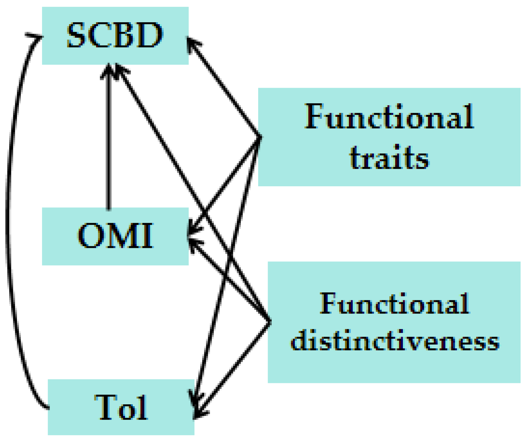
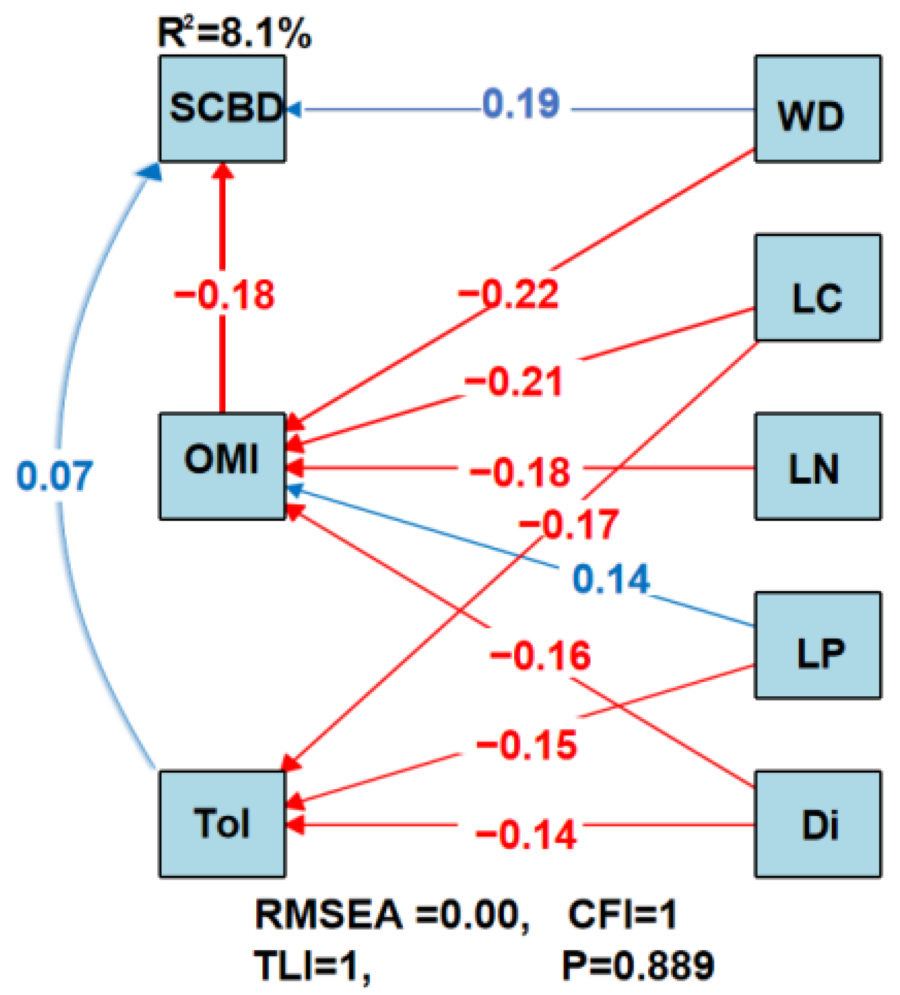
2.4.3. Statistical Modeling

In this study, we constructed a structural equation modeling (SEM) hypothesis model based on the conceptual framework (Figure 1) [26,32]. The exogenous variables in the model include functional distinctiveness and plant functional traits, while the endogenous variables are species ecological niche characteristics and SCBD. We separately fitted SEM models for SCBD based on abundance data and SCBD based on presence–absence data. During model selection, we compared the RMSEA (root mean square error of approximation), CFI (comparative fit index), and TFI (Tucker–Lewis index) values to ensure a better fit [34]. We retained paths with p < 0.05 during model fitting. The model aims to explore whether functional traits, functional distinctiveness, and niche characteristics (including niche location and niche breadth) have an impact on SCBD.

2.4.4. Beta Regression to Analyze

Because species data vary between 0 and 1, this study applied β regression to analyze changes in SCBD. Specifically, SCBD was treated as the response variable, while species indicators (species abundance and occupancy) served as predictor factors [35].

$$g\left(u_t\right)=\sum _{i=1}^k{x}_{ti}{\beta }_i={\eta }_t$$

(14)

Among them, ${\beta }_i$ is a vector of unknown regression parameters, $x_{ti}$ is a vector of regression factors (or independent variables or covariates), ${\eta }_t$ is the linear predictor, t is the t-th observation, $u_t$ represents the mean of the response variable, and k is the k-th sample size. In this study, β regression is analyzed using the “betareg” package in R 4.3.3 [32,35].

3. Results

3.1. Distribution of SCBD

In both abundance-based and presence–absence data, the average value of SCBD is 0.0048 (Figure 2). This study used a beta regression model to analyze SCBD based on abundance data and presence–absence data. The results revealed that under abundance conditions, species richness and occupancy were significantly linearly related to SCBD (Figure 3a,b). However, under presence–absence conditions, there was a pronounced hump-shaped relationship between abundance, occupancy, and SCBD (Figure 3c,d). Under abundance conditions, the model coefficients for abundance and occupancy are −0.0002 and 0.0090, respectively (

Table 2. Beta regression model analysis between SCBD and abundance and occupancy based on abundance data and presence–absence data.

Data Situation	Item	Coefficient	p Value
Abundance data	Abundance	−0.0002	p < 0.001
	Occupancy	0.0090	p < 0.001
	Intercept	−5.8537	p < 0.001
Presence–absence data	Abundance	0.0002	p < 0.001
	Occupancy	0.0068	p < 0.001
	Intercept	−6.1157	p < 0.001

). Under presence–absence conditions, the model coefficients for abundance and occupancy are 0.0002 and 0.0068 (Table 2).

3.2. Impact of Species Traits on SCBD

In SEM constructed based on abundance, SEM supports the indirect impact of functional distinctiveness and plant functional traits on SCBD by influencing species ecological niche characteristics. Specifically, OMI and Tol directly affect SCBD. OMI (with a standardized path coefficient of −0.18) has a negative effect on SCBD, while Tol (with a standardized path coefficient of 0.07) has a positive effect. Additionally, there is a certain correlation between functional distinctiveness (Di), plant functional traits (WD, LC, LN, and LP), and species ecological niche characteristics (OMI and Tol), which further indirectly influence SCBD. Notably, functional distinctiveness negatively affects species ecological niche characteristics (OMI and Tol). In summary, functional distinctiveness, functional traits, and ecological niche characteristics explain 8.1% of the variation in abundance-based SCBD (Figure 4).

In SEM constructed based on presence–absence, the variables OMI, Tol, and WD have direct effects on SCBD. Specifically, WD (with a standardized path coefficient of 0.24) and Tol (with a standardized path coefficient of 0.31) positively influence SCBD, while OMI (with a standardized path coefficient of −0.39) has a negative impact on SCBD. Additionally, LC negatively affects species ecological niche characteristics (OMI and Tol), indirectly influencing SCBD. The coefficient of determination (R²) for SCBD reaches 29.2% (Figure 5).

4. Discussion

4.1. Distribution of SCBD

In this study, we found that the average value of species co-occurrence and beta diversity was 0.0048 under both abundance data and presence–absence data. Specifically, in the case of abundance, there was a significant linear relationship between species abundance and occupancy and SCBD. However, under the presence–absence scenario, these three factors exhibited a pronounced hump-shaped relationship. This is consistent with the results of Wang et al. [9] in their study of subtropical forests in southern China. On one hand, our study found a significant linear relationship between species abundance and occupancy rate with respect to SCBD under abundance conditions. This result is consistent with the findings of Heino and Grönroos [8], suggesting that species with higher abundance and occupancy rates may be more inclined to coexist with other species, resulting in lower SCBD values. On the other hand, our study revealed a pronounced hump-shaped relationship between abundance, occupancy rate, and SCBD based on presence–absence data. This finding aligns with Xia et al.’s [12] investigation of spatial patterns of β-diversity contributions in fish communities and species in river ecosystems. They also observed a hump-shaped relationship between presence–absence SCBD and occupancy rate, as well as total abundance. The pronounced hump-shaped relationship between abundance, occupancy rate, and SCBD may be attributed to various factors such as adaptability of biological populations, species interactions, and environmental heterogeneity. To gain a deeper understanding of the specific mechanisms underlying this relationship, further research and analysis are needed.

4.2. Impact of Species Ecological Niche Characteristics on SCBD

This research found that species niche characteristics directly influence SCBD values, and the niche position and niche width have opposite effects on SCBD. This result aligns with the findings of Wang et al. [9], indicating that the direct impact of species ecological niche characteristics (including niche position and breadth) on SCBD is opposite. Szabó et al. [36] also found that species ecological niche characteristics are key factors directly influencing SCBD values.

The ecological niche position has a negative impact on SCBD. Studies by Xia et al. [12] and Wang et al. [9] have both found a negative correlation between niche position and SCBD. In this study, using structural equation modeling (SEM) based on abundance data and presence–absence data, we reconfirmed this relationship, showing that species occupying central ecological niches tend to have higher SCBD values [10]. The ecological niche position hypothesis posits that species capable of adapting to the most common environmental conditions in a specific area should be the most abundant [18]. In other words, a species’ abundance is closely related to its ecological niche position. In their study, Castaño Quintero et al. [37] investigated the effects of niche position and breadth on population abundances in 47 bird species belonging to the Parulidae family. The results indicated a negative correlation between niche position and both mean abundance and maximum abundance. Therefore, the negative correlation between ecological niche position and species abundance may lead to a negative correlation between ecological niche position and SCBD values.

A positive correlation between ecological niche width and SCBD was found in this study, which contrasts with the results from Da Silva and Xia [10,12], who found no significant correlation between ecological niche width and SCBD. In a biome, species with larger niche widths tend to exhibit higher SCBD values, and species with larger niche widths contribute more significantly to overall β-diversity [9]. The relationship between Tol and SCBD is positively correlated. This relationship may vary depending on the region and species group in terms of the association between niche width and species abundance [38]. Additionally, species with larger niche widths may exhibit greater abundance variations across different habitats [8]. Therefore, inferring the relationship between niche width and SCBD cannot rely solely on the link between niche width and species richness, but should consider more deeply how species are able to adapt to diverse environmental conditions.

4.3. The Impact of Plant Functional Traits on SCBD

This study found that functional traits indirectly influence SCBD through species ecological niche characteristics. Previous research has indicated that species functional traits are either unrelated or weakly correlated with SCBD [8,10], possibly considering only the direct effects of traits and overlooking indirect effects. This study found that functional traits indirectly influence SCBD values through species ecological niche characteristics in both abundance-based SCBD and presence–absence-based SCBD SEM. This may be due to a certain correlation between biological traits and species ecological niche characteristics [18]. Additionally, functional traits serve as the foundation of SCBD models, as they are related to species occupancy and abundance [12]. Ecological niche position and width are key factors determining species occupancy and abundance [18], suggesting that functional traits may also have an impact on SCBD. Our findings provide a scientific basis for effective biodiversity conservation and ecosystem management strategies for tropical karst forests.

4.4. The Impact of Functional Distinctiveness on SCBD

Functional distinctiveness indirectly affects SCBD values. Wang et al. [9] found that functional distinctiveness influences SCBD values in an indirect manner, and its overall impact on abundance-based SCBD and presence–absence-based SCBD is negative. Differently, this study found that functional distinctiveness indirectly affects SCBD only under abundance-based conditions, and the impact is negative. This may be because species with unique trait combinations (i.e., higher functional distinctiveness) occupy marginal ecological niches and maintain narrower niche widths, resulting in a smaller contribution to overall β-diversity [9]. Functional distinctiveness negatively impacts ecological niche position and ecological niche width (Figure 4), suggesting that species with unique functions in the study area may be constrained in their ecological position and resource utilization patterns within the ecosystem. However, under presence–absence conditions, functional distinctiveness does not directly affect ecological niche position, ecological niche width, or overall β-diversity (Figure 5). This discrepancy may arise from stochastic diffusion limiting functional distinctiveness, which might not be directly associated with ecological niche position or width [39]. Therefore, functional distinctiveness under presence–absence conditions does not impact SCBD, but this does not imply that functional distinctiveness lacks value in ecological research.

In this study, we found that in SEM based on presence–absence data, the coefficient of determination (R²) for SCBD reaches 29.2% (Figure 5), which is significantly higher than the SEM constructed using abundance data, where SCBD’s R² is only 8.1% (Figure 4). This difference may be attributed to various ecological processes influencing species distribution patterns [40]. For instance, processes such as habitat selection and species interactions might be more easily captured by models using presence–absence data, whereas in abundance data, these processes may be less apparent due to other factors like environmental heterogeneity and species competition [40]. Therefore, investigating the impact of species ecological niche characteristics, functional distinctiveness, and plant traits on SCBD in SEM based on presence–absence data can provide deeper insights into the ecological mechanisms underlying species distribution patterns and help predict and interpret species distributions under different environmental conditions.

Research has found that β-diversity plays a crucial role in understanding changes in biodiversity and their impact on ecosystem functioning [41]. Specifically, plant β-diversity has a strong positive effect on ecosystem multifunctionality, such as primary productivity and soil carbon sequestration [42]. So, increasing total β-diversity may be beneficial for ecosystem functioning. From a basic ecological, conservation, and biological assessment perspective, understanding the determinants of SCBD is crucial. Research indicates that species contribute to SCBD by revealing the roles of different species in shaping inter-community differences. Species with higher SCBD may play a key role in forming these differences, which is significant for maintaining biodiversity and ecological processes [36]. Therefore, species contributing significantly to overall β-diversity should receive special attention. These species may positively impact primary functions of communities, such as primary productivity. By identifying species with higher SCBD, we can not only better understand the key focus areas for biodiversity conservation but also gain insights into which species significantly influence community assembly and diversity patterns. Additionally, species with lower SCBD may provide unique functions due to their distinct trait combinations, making them equally worthy of attention. This implies that in ecological conservation and restoration efforts, it is essential to consider not only the overall diversity level but also the individual species that compose this diversity and their unique functions.

5. Conclusions

This study explores the relationship between species occupancy, abundance, species ecological niche characteristics (niche position and niche width), functional traits, and functional distinctiveness with SCBD. The research findings indicate that these species characteristics are correlated with SCBD. Linking local community β-diversity to species functional traits contributes to a better understanding of the mechanisms underlying β-diversity formation, which is crucial for comprehending biodiversity variation and its practical implications. This study found that SEM models based on the presence–absence data provide higher explanatory power, offering a new perspective for understanding species distribution patterns. Future research can further explore the applicability of different data types in various ecological contexts and optimize models to handle data uncertainty and complexity. However, relying solely on SCBD to determine which species should receive special protection may overlook the quality of biodiversity conservation. Clarifying the link between functional traits and SCBD is essential for developing a more comprehensive and effective biodiversity conservation strategy. Therefore, future research should delve into the unique functions provided by species with distinct trait combinations and explore the direct connection between SCBD and ecosystem functioning.

References

1. White, H.J.; McKeon, C.M.; Pakeman, R.J.; Buckley, Y.M. The contribution of geographically common and rare species to the spatial distribution of biodiversity. Glob. Ecol. Biogeogr. 2023, 32, 1730–1747. [Google Scholar] [CrossRef]
2. Whittaker, R.H. Vegetation of the Siskiyou mountains, Oregon and California. Ecol. Monogr. 1960, 30, 279–338. [Google Scholar] [CrossRef]
3. Legendre, P.; De Cáceres, M. Beta diversity as the variance of community data: Dissimilarity coefficients and partitioning. Ecol. Lett. 2013, 16, 951–963. [Google Scholar] [CrossRef]
4. Zhang, X.; Liu, S.; Wang, J.; Huang, Y.; Freedman, Z.; Fu, S.; Liu, K.; Wang, H.; Li, X.; Yao, M. Local community assembly mechanisms shape soil bacterial β diversity patterns along a latitudinal gradient. Nat. Commun. 2020, 11, 5428. [Google Scholar] [CrossRef] [PubMed]
5. Santos, F.; Lima, M.G.M.; Espinosa, S.; Ahumada, J.A.; Jansen, P.A.; Spironello, W.R.; Hurtado, J.; Juen, L.; Peres, C.A. Site and species contribution to β-diversity in terrestrial mammal communities: Evidence from multiple Neotropical forest sites. Sci. Total Env. Environ. 2021, 789, 147946. [Google Scholar] [CrossRef] [PubMed]
6. Legendre, P.; Borcard, D.; Peres-Neto, P.R. Analyzing beta diversity: Partitioning the spatial variation of community composition data. Ecol. Monogr. 2005, 75, 435–450. [Google Scholar] [CrossRef]
7. Myers, J.A.; LaManna, J.A. The promise and pitfalls of β-diversity in ecology and conservation. J. Veg. Sci. 2016, 27, 1081–1083. [Google Scholar] [CrossRef]
8. Heino, J.; Grönroos, M. Exploring species and site contributions to beta diversity in stream insect assemblages. Oecologia 2017, 183, 151–160. [Google Scholar] [CrossRef] [PubMed]
9. Wang, W.; Jiang, Y.; Li, B.; Luo, W.; Chu, C.; Wang, Y. How does functional distinctiveness affect single species contribu-tion to β diversity? Evidence from a subtropical forest plot in southern China. Ecol. Indic. 2023, 146, 109736. [Google Scholar] [CrossRef]
10. Da Silva, P.G.; Hernández, M.I.M.; Heino, J. Disentangling the correlates of species and site contributions to beta diversity in dung beetle assemblages. Divers. Distrib. 2018, 24, 1674–1686. [Google Scholar] [CrossRef]
11. Krasnov, B.R.; Shenbrot, G.I.; Warburton, E.M.; Van Der Mescht, L.; Surkova, E.N.; Medvedev, S.G.; Pechnikova, N.; Er-molova, N.; Kotti, B.K.; Khokhlova, I.S. Species and site contributions to β-diversity in fleas parasitic on the Palearctic small mammals: Ecology, geography and host species composition matter the most. Parasitology 2019, 146, 653–661. [Google Scholar] [CrossRef] [PubMed]
12. Xia, Z.; Heino, J.; Yu, F.; He, Y.; Liu, F.; Wang, J. Spatial patterns of site and species contributions to β diversity in river-ine fish assemblages. Ecol. Indic. 2022, 145, 109728. [Google Scholar] [CrossRef]
13. De Bello, F.; Lavorel, S.; Díaz, S.; Harrington, R.; Cornelissen, J.H.; Bardgett, R.D.; Berg, M.P.; Cipriotti, P.; Feld, C.K.; He-ring, D. Towards an assessment of multiple ecosystem processes and services via functional traits. Biodivers. Conserv. 2010, 19, 2873–2893. [Google Scholar] [CrossRef]
14. Violle, C.; Thuiller, W.; Mouquet, N.; Munoz, F.; Kraft, N.J.B.; Cadotte, M.W.; Livingstone, S.W.; Mouillot, D. Functional Rarity: The Ecology of Outliers. Trends Ecol. Evol. 2017, 32, 356–367. [Google Scholar] [CrossRef] [PubMed]
15. Kondratyeva, A.; Knapp, S.; Durka, W.; Kühn, I.; Vallet, J.; Machon, N.; Martin, G.; Motard, E.; Grandcolas, P.; Pavoine, S. Urbanization Effects on Biodiversity Revealed by a Two-Scale Analysis of Species Functional Uniqueness vs. Redundancy. Front. Ecol. Evol. 2020, 8, 73. [Google Scholar] [CrossRef]
16. Gaüzère, P.; Blonder, B.; Denelle, P.; Fournier, B.; Grenié, M.; Delalandre, L.; Münkemüller, T.; Munoz, F.; Violle, C.; Thuiller, W. The functional trait distinctiveness of plant species is scale dependent. Ecography 2023, 2023, e6504. [Google Scholar] [CrossRef]
17. Grenié, M.; Denelle, P.; Tucker, C.M.; Munoz, F.; Violle, C. funrar: An R package to characterize functional rarity. Divers. Distrib. 2017, 23, 1365–1371. [Google Scholar] [CrossRef]
18. Marino, N.A.; Cereghino, R.; Gilbert, B.; Petermann, J.S.; Srivastava, D.S.; de Omena, P.M.; Bautista, F.O.; Guzman, L.M.; Romero, G.Q.; Trzcinski, M.K. Species niches, not traits, determine abundance and occupancy patterns: A multi-site syn-thesis. Global Ecol. Biogeogr. 2020, 29, 295–308. [Google Scholar] [CrossRef]
19. Guo, Y.; Wang, B.; Mallik, A.U.; Huang, F.; Xiang, W.; Ding, T.; Wen, S.; Lu, S.; Li, D.; He, Y.; et al. Topo-graphic species–habitat associations of tree species in a heterogeneous tropical karst seasonal rain forest, China. J. Plant Ecol. 2016, 10, 450–460. [Google Scholar]
20. Guo, Y.; Chen, H.Y.H.; Mallik, A.U.; Wang, B.; Li, D.; Xiang, W.; Li, X. Predominance of abiotic drivers in the relationship between species diversity and litterfall production in a tropical karst seasonal rainforest. For. Ecol. Manag. 2019, 449, 117452. [Google Scholar] [CrossRef]
21. Mittermeier, R.A.; Turner, W.R.; Larsen, F.W.; Brooks, T.M.; Gascon, C. Global biodiversity conservation: The critical role of hotspots. In Biodiversity Hotspots: Distribution and Protection of Conservation Priority Areas; Springer: Berlin/Heidelberg, Germany, 2011; pp. 3–22. [Google Scholar]
22. Xingming, Z.; Bin, W.; Ting, C.; Yili, G.; Xiankun, L. Revealing the relative importance among plant species, slope posi-tions, and soil types on rhizosphere microbial communities in northern tropical karst and non-karst seasonal rainforests of China. Front. Microbiol. 2023, 14, 1103550. [Google Scholar]
23. Ruixia, M.; Jianxing, L.; Yili, G.; Bin, W.; Wusheng, X.; Dongxing, L.; Fuzhao, H.; Fang, L.; Shujun, W.; Shuhua, L.; et al. Re-cruitment dynamics in a tropical karst seasonal rain forest: Revealing complex processes from spatial patterns. For. Ecol. Manag. 2024, 553, 121610. [Google Scholar]
24. Guo, Y.; Wang, B.; Li, D.; Mallik, A.U.; Xiang, W.; Ding, T.; Wen, S.; Lu, S.; Huang, F.; He, Y.; et al. Effects of topography and spatial processes on structuring tree species composition in a diverse heterogeneous tropical karst seasonal rainforest. Flora 2017, 231, 21–28. [Google Scholar] [CrossRef]
25. Hu, G.; Pang, Q.; Hu, C.; Xu, C.; Zhang, Z.; Zhong, C. Beta Diversity Patterns and Determinants among Vertical Layers of Tropical Seasonal Rainforest in Karst Peak-Cluster Depressions. Forests 2024, 15, 365. [Google Scholar] [CrossRef]
26. Grace, J.B. Structural Equation Modeling and Natural Systems; Cambridge University Press: Cambridge, UK, 2006. [Google Scholar]
27. Bai, K.; Lv, S.; Ning, S.; Zeng, D.; Guo, Y.; Wang, B. Leaf nutrient concentrations associated with phylogeny, leaf habit and soil chemistry in tropical karst seasonal rainforest tree species. Plant Soil. 2019, 434, 305–326. [Google Scholar] [CrossRef]
28. Pérez-Harguindeguy, N.; Díaz, S.; Garnier, E.; Lavorel, S.; Poorter, H.; Jaureguiberry, P.; Bret-Harte, M.S.; Cornwell, W.K.; Craine, J.M.; Gurvich, D.E.; et al. New handbook for standardised measurement of plant functional traits worldwide. Aust. J. Bot. 2013, 61, 167. [Google Scholar] [CrossRef]
29. Roberts, D.W.; Cooper, S.V. Concepts and techniques of vegetation mapping. In Land Classification Based on Vegetation; Applications for Resource Management: Moscow, Russia, 1989; pp. 90–96. [Google Scholar]
30. Scrimgeour, C. Soil Sampling and Methods of Analysis, 2nd ed.; Carter, M.R., Gregorich, E.G., Eds.; CRC Press: Boca Raton, FL, USA, 2008; ISBN 978-0-8593-3586-0. [Google Scholar]
31. Dolédec, S.; Chessel, D.; Carpentier, C.G. Niche Separation in Community Analysis: A New Method. Ecology 2000, 81, 2914–2927. [Google Scholar] [CrossRef]
32. Team, R.C. R: A Language and Environment for Statistical Computing; R Foundation for Statistical Computing: Vienna, Austria, 2024. [Google Scholar]
33. Dray, S.; Dufour, A. The ade4 package: Implementing the duality diagram for ecologists. J. Stat. Softw. 2007, 22, 1–20. [Google Scholar] [CrossRef]
34. Xia, Y.; Yang, Y. RMSEA, CFI, and TLI in structural equation modeling with ordered categorical data: The story they tell depends on the estimation methods. Behav. Res. Methods 2019, 51, 409–428. [Google Scholar] [CrossRef]
35. Cribari-Neto, F.; Zeileis, A. Beta Regression in R. J. Stat. Softw. 2010, 34, 1–24. [Google Scholar] [CrossRef]
36. Szabó, B.; Lengyel, E.; Padisák, J.; Stenger-Kovács, C. Benthic diatom metacommunity across small freshwater lakes: Driving mechanisms, β-diversity and ecological uniqueness. Hydrobiologia 2019, 828, 183–198. [Google Scholar] [CrossRef]
37. Castaño Quintero, S.; Velasco, J.; González Voyer, A.; Martínez Meyer, E.; Yáñez Arenas, C. Niche position and niche breadth effects on population abundances: A case study of New World Warblers (Parulidae). Ecol. Evol. 2024, 14, e11108. [Google Scholar] [CrossRef] [PubMed]
38. Vela Díaz, D.M.; Blundo, C.; Cayola, L.; Fuentes, A.F.; Malizia, L.R.; Myers, J.A.; Pither, J.; Pither, J. Untangling the im-portance of niche breadth and niche position as drivers of tree species abundance and occupancy across biogeographic re-gions. Glob. Ecol. Biogeogr. 2020, 29, 1542–1553. [Google Scholar] [CrossRef]
39. François, M.; Klausmeier, C.A.; Pierre, G.; Gaurav, K.; Elena, L.; Nicolas, M.; Annette, O.; Wilfried, T.; Algar, A.C.; Arnaud, A.; et al. The ecological causes of functional distinctiveness in communities. Ecol. Lett. 2023, 26, 1452–1465. [Google Scholar]
40. Zhu, Y.J.; Shan, D.; Zhang, X.; Liu, Y.S.; Shi, Z.J.; Yang, X.H. Advances in joint species distribution models to re-veal community structure and its environmental response. Chin. J. Appl. Ecol. 2018, 29, 4217–4225. [Google Scholar]
41. Mori, A.S.; Isbell, F.; Seidl, R. β-diversity, community assembly, and ecosystem functioning. Trends Ecol. Evol. 2018, 33, 549–564. [Google Scholar] [CrossRef] [PubMed]
42. van Der Plas, F.; Manning, P.; Soliveres, S.; Allan, E.; Scherer-Lorenzen, M.; Verheyen, K.; Wirth, C.; Zavala, M.A.; Am-poorter, E.; Baeten, L. Biotic homogenization can decrease landscape-scale forest multifunctionality. Proc. Natl. Acad. Sci. USA 2016, 113, 3557–3562. [Google Scholar] [CrossRef]
Figure 1. Conceptual framework linking functional traits, functional distinctiveness, ecological niche characteristics, and SCBD, ecological niche position (OMI) and ecological niche breadth (Tol).
Forests 15 01125 g001
Figure 2. Histogram of SCBD values based on abundance (blue) and presence–absence (green). The red dashed line represents the average SCBD under abundance and presence–absence conditions.
Forests 15 01125 g002
Figure 3. Scatterplot and marginal histograms of species contribution to beta diversity (SCBD) in relation to abundance and occupancy. Panels (a,b) represent abundance conditions. Panels (c,d) represent presence–absence conditions. The regression models were fitted between response variables and each predictor variable.
Forests 15 01125 g003
Figure 4. Impact of different variables on species compositional beta diversity (SCBD) based on abundance. Note: The values represent estimated standardized path coefficients, indicating the strength and magnitude of direct and indirect effects of variables on SCBD. Arrows denote important relationships between variables (p < 0.05). Blue arrows indicate positive correlations, while red arrows indicate negative correlations. OMI stands for ecological niche position, Tol represents ecological niche width, and Di refers to functional distinctiveness; WD stands for wood density, LC represents leaf carbon content, LN corresponds to leaf nitrogen content, and LP denotes leaf phosphorus content.
Forests 15 01125 g004
Figure 5. Interaction effects of different variables on species compositional beta diversity (SCBD) based on presence–absence. Note: The values represent estimated standardized path coefficients, indicating the strength and magnitude of direct and indirect effects of variables on SCBD. Arrows denote important relationships between variables (p < 0.05). Blue arrows indicate positive correlations, while red arrows indicate negative correlations. OMI stands for ecological niche position, Tol represents ecological niche width, and Di refers to functional distinctiveness; WD stands for wood density and LC represents leaf carbon content.
Forests 15 01125 g005