Stress Wave Hybrid Imaging for Detecting Wood Internal Defects under Sparse Signals

Abstract

Stress wave technology is very suitable for detecting internal defects of standing trees, logs, and wood and has gradually become the mainstream technology in this research field. Usually, 12 sensors are positioned equidistantly around the cross-section of tree trunks in order to obtain enough stress wave signals. However, the arrangement of sensors is time-consuming and laborious, and maintaining the accuracy of stress wave imaging under sparse signals is a challenging problem. In this paper, a novel stress wave hybrid imaging method based on compressive sensing and elliptic interpolation is proposed. The spatial structure of the defective area is reconstructed by using the advantages of compressive sensing in sparse signal representation and solution of stress waves, and the healthy area is reconstructed by using the elliptic space interpolation method. Then, feature points are selected and mixed for imaging. The comparative experimental results show that the overall imaging accuracy of the proposed method reaches 89.7%, and the high-quality imaging effect can be guaranteed when the number of sensors is reduced to 10, 8, or even 6.

1. Introduction

Wood is an important biological resource and material. How to effectively detect the internal defects of wood without destroying wood is meaningful research, which can help protect trees and ancient wooden buildings and improve the utilization rate of logs [1,2]. At present, researchers in this field widely use stress wave signals to analyze and assess internal defects in wood [3,4,5]. Stress wave technology has the advantages of good portability, slight damage to wood, strong anti-interference ability, no harm to the human body, and convenience of use [6]. It reflects the internal structural characteristics of the tested object through the difference in stress wave propagation velocity in different media [7,8]. In the application of this technology, a sensor placed in a certain position on the cross-section of the tree trunk is used to generate stress wave signals, and the other stress wave sensors placed annularly on the cross-section of the tree trunk are used to receive stress wave signals propagating in different directions inside wood. Then, by analyzing the time difference between the received signal and the excitation signal, the propagation velocity distribution matrix of the stress wave is established. Finally, according to the difference in stress wave propagation velocity in different media (internal defects and healthy wood), pattern recognition can be used to assess the internal health of wood [9,10,11]. Furthermore, stress wave imaging methods such as spatial interpolation can be used to reconstruct the image of wood internal defects, so as to intuitively reflect the location, size, and shape of the defects [12,13,14].

In the process of two-dimensional imaging of wood internal defects by using stress wave signals, reconstructing high-quality defect images by using limited stress wave signals is the key step [15,16]. In order to solve this problem, researchers have proposed many stress wave imaging algorithms. Arciniegas et al. [17] proposed an imaging method by improving the acoustic velocity determination. In their work, the effect of the signal dynamic on the velocity determination was studied, the validity range of each computation method was determined, and the behavior between a homogeneous material and wood was compared. Huan et al. [18] computed the wave velocity distribution of the grid cells of wood cross-sections by the least square QR decomposition (LSQR) iterative inversion, and the error correction mechanism was used to optimize the image of defects, which effectively reduced the error of stress wave velocity inversion calculation. Liu et al. [19] proposed a stress wave imaging method based on a mixed wave propagation model, which can detect the decay defects in trees. Qiu et al. [20] developed a tomographic technique based on the use of both mechanical waves (i.e., stress waves and acoustic waves) and electromagnetic waves (i.e., laser beams) for evaluating the defects in tree trunks. Their technique can achieve a more accurate and reliable detection of internal defects in tree systems, especially if the internal defects are close to the free surface.

Among existing stress wave imaging algorithms, an algorithm called ellipse-based spatial interpolation (EBSI for short) can achieve relatively good 2D imaging results of internal defects in wood using stress wave signals and has become a classic algorithm in wood defects detection field [21,22,23]. The propagation mechanism of stress waves in wood has not been fully understood, because wood is an anisotropic material with a special internal structure [24,25,26]. Against this background, the EBSI method assumes that the propagation path of the stress wave in wood is a straight line, visualizes the stress wave propagation velocity matrix as shown in Figure 1a, and then reconstructs the internal defects using spatial interpolation. In order to distinguish the defective area from the healthy wood area, the stress wave velocity can be visualized in different colors [27,28]. The greater the wave velocity, the greener the color corresponding to the straight line, which means that the stress wave has passed through the healthy area; On the contrary, the smaller the wave velocity value, the redder the color corresponding to the straight line, which means that the stress wave has passed through the defect area (if it encounters a cavity defect, the stress wave will propagate around the defect area, resulting in an increase in the propagation time between two sensors). As shown in Figure 1b, the basic idea of the EBSI method is to ellipticize each stress wave propagation straight line and estimate each grid point in the imaging area (as shown in Figure 1c) using elliptic space interpolation. Specifically, an ellipse is generated adaptively according to the length of the propagation straight line (which becomes the affected zone), and then the velocity distribution value of each grid point in the imaging area is traversed and calculated by the colors of all ellipses covering the grid point. Different interpolation strategies such as ellipse shape design and grid point estimation have been proposed based on EBSI [20,22,23,29,30,31].

In order to obtain good imaging results, traditional stress wave imaging methods, including EBSI, need enough signals as input data [32,33]. Therefore, at present, the algorithms in this field use as many sensors as possible to collect signals (generally 12 sensors) [34]. However, the sensor arrangement process is time-consuming and labor-intensive, reducing the number of sensors can greatly reduce the time spent on stress wave signal acquisition, thus effectively improving the practical efficiency and ease of use of stress wave imaging technology. Therefore, if the number of sensors can be reduced for signal acquisition, sparse signals can be used to achieve stress wave imaging, while also ensuring high-quality imaging results of wood internal defects; it is bound to further promote the development of stress wave imaging technology. Obviously, detecting wood internal defects under sparse signals puts forward higher requirements for imaging algorithms. To address this challenging issue, this paper proposes a novel stress wave hybrid imaging algorithm based on compressive sensing and elliptical interpolation. We combined compressive sensing theory with stress wave imaging, leveraging the advantages of sparse representation and solution of stress wave signals in compressive sensing, while also leveraging the advantages of traditional spatial interpolation algorithms in reconstructing healthy wood area, to reconstruct images of internal defects in tree trunks. In the experiment, as the number of sensors gradually decreased, the effectiveness of the proposed algorithm was tested through both simulated and real samples, and the imaging results were quantitatively analyzed using multiple indicators.

2. Materials and Methods

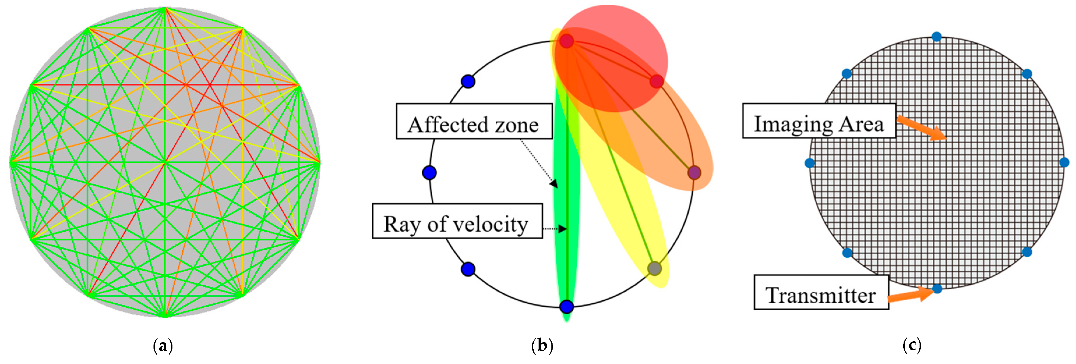
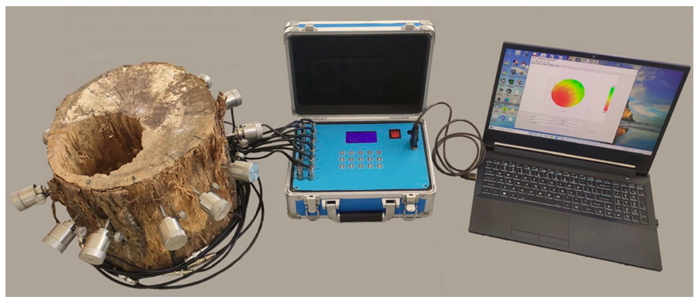
2.1. Materials and Data Acquisition

The stress wave signal acquisition apparatus named Wopecker (v2.0, Hangzhou, China) was independently designed and developed by our research group in the previous work. As shown in Figure 2, The apparatus consists of 12 piezoelectric-type sensors, a stress wave signal processing box, a percussion hammer, and several data transmission lines. The working parameters of the device are as follows: the measurement range of stress wave propagation time is 0–65,535 μs; the measurement range of stress wave propagation speed is 0–3000 m/s; the time resolution is 1 microsecond; the number of sensor channels is 12; the maximum pressure that the sensor can withstand is 500 N; can be externally connected to a working voltage of DC5V-DC12V; can be connected to a working voltage of 4.2 V lithium battery internally; the time interval between a single measurement is less than 1.5 s.

As shown in Figure 3, when the stress wave signal is collected, a group of sensors is arranged on a certain cross-section of wood at an equal distance. As a sensor is struck, a stress wave signal is generated and propagated in the wood, the other sensors will receive the stress wave signal, and the propagation time from the signal source to the receiving sensors is estimated by Digital Signal Processing technology (short time energy and double threshold detection are used to estimate the propagation time of stress wave). Then, the signal processing box transmits the time matrix to the computer (CPU: 2.10 GHz, RAM: 8 GB) through a USB connection. The self-developed software (v2.0, Hangzhou, China) has the following functions: input of sensor position information as shown in Figure 2e; display of sensor distance matrix; display of propagation time matrix; display of propagation speed matrix; display of stress wave paths as shown in Figure 2f; display of two-dimensional imaging results; port settings; and printing of report forms, etc. This paper focuses on the stress wave imaging algorithm, and the specific estimation method of stress wave propagation time has been published by the members of our group in the previous research [35].

Both simulation samples and real samples were used in the experiment. As shown in Figure 4, we designed four kinds of simulated samples to evaluate the performance of the proposed algorithm. The spatial distribution forms of simulated defects include overlapping double-circle distribution, single-circle distribution, edge semi-circle distribution, and double-edge semi-circle distribution. In addition, two tree trunks were used in the experiment, including a Pecan tree sample with cavity defects and a Camphor tree sample with cavity defects. The two tree trunks are both hard wood, and the moisture content of them is between 10%–20%. The proportion of defective area in both of the two tree trunks is about 5%.

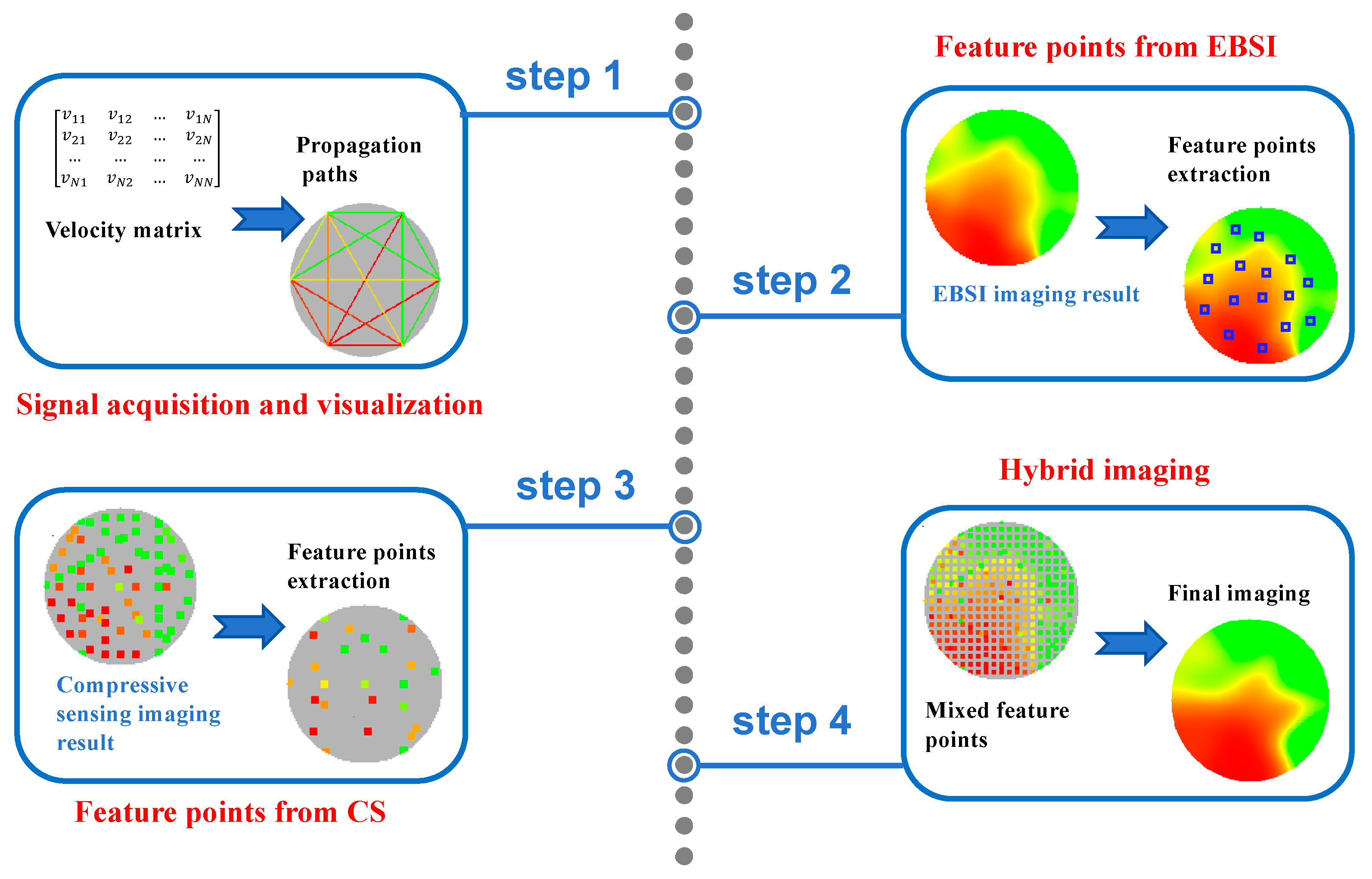
2.2. Proposed Imaging Method

Compressed sensing theory is a method based on signal sparse representation and approximation theory [36], which has been applied in many research fields in recent years. The principle of compressive sensing can be expressed as follows:

$$y=\Phi x$$

(1)

where x represents the original digital signal, which needs to be sparse (or sparse in a transform domain); y is the compressed signal representation; and $\Phi$ stands for measurement matrix. The compressive sensing method uses the convex optimization method to solve the underdetermined equations and recover the original signal x with high probability under the condition that the measured value y is known through a small number of observations. In general, the natural signal x itself is not sparse, and it needs to be expressed sparsely on some sparse basis:

$$x=\Psi \alpha$$

(2)

where $\Psi$ is a sparse basis matrix and $\alpha$ is a sparse coefficient with only K non-zero values. In this way, through Formulas (1) and (2), we can obtain the following:

$$y=\Phi \Psi \alpha =\Phi \prime \alpha$$

(3)

where $\Phi \prime$ is called the sensing matrix, the approximate value $\alpha \prime$ of $\alpha$ is solved, and then the approximate value x′ of the original signal can be obtained. The signal acquisition process based on compressive sensing is a linear projection process. A vector y (M × 1) can recover K non-zero values of $\alpha$, and the original signal can be effectively recovered through a small number of observations.

According to the basic principle of compressed sensing, the key steps of this method are as follows: effective sparse representation of the original signal, design of measurement matrix (to reduce the dimension while ensuring the minimum information loss of the original signal x), and design of signal recovery algorithm. Among them, the measurement matrix can usually be a random matrix, and the problem of solving underdetermined equations can be transformed into an l₁ norm-constrained optimization problem [37,38]. According to Formula (2), the purpose of designing this step in the compressive sensing principle is to ensure that the original signal is sparse, so as to ensure that the underdetermined equations can be effectively solved.

Compressed sensing can be used for image and video sampling and reconstruction, which can significantly reduce the sampling rate while maintaining high reconstruction quality. In medical imaging technologies such as CT, MRI, and PET, compressive sensing can significantly reduce scanning time and radiation dose while maintaining high imaging quality [39,40]. In radar and remote sensing systems, compressive sensing can be used to reduce the number of array components and improve imaging resolution [41]. In electrical imaging technologies such as ECT and ERT, the image reconstruction algorithms are required fast and accurate, and compressive sensing is often used to reconstruct a higher-quality image with fewer iteration steps (shorter elapsed time) [42,43]. These methods are all applications of compressive sensing in other imaging research fields, which fully demonstrates the effectiveness of combining this method with imaging technology. Although there have been no reports on the application of compressive sensing in stress wave imaging, the significance of compressive sensing methods lies in reconstructing high-quality images or matrices based on sparse signals, which is consistent with the research objective of this paper. Therefore, compressive sensing is worth considering for stress wave imaging. The blank grids in the imaging area used for image reconstruction are sparse. Based on the principle of compressive sensing, the following formula for solving the spatial distribution of stress wave velocity can be defined as follows:

$$T=LS=L\times \frac{1}{V}$$

(4)

where L represents the length of the stress wave propagation path, T represents the propagation time of the stress wave, V represents the propagation speed of the stress wave, and S is the reciprocal of the wave velocity value of the stress wave. Obviously, Formula (4) is similar to Formula (3) for compressive sensing. When the size of the blank grid in the imaging area is small enough, S is sparse, so the stress wave signal acquisition process (the signal acquisition process after the electronic hammer hits a sensor once) can be expressed by the above formula. Further, the above formula is expressed in matrix form as follows:

$$\left(\begin{array}{c}{t}_1\\ t_2\\ \dots \\ t_{\mathrm{M}}\end{array}\right)=\left(\begin{array}{cccc}{l}_{11}& l_{12}& \dots & l_{1\mathrm{N}}\\ l_{21}& l_{22}& \dots & l_{2\mathrm{N}}\\ \dots & \dots & \dots & \dots \\ l_{\mathrm{M}1}& l_{\mathrm{M}2}& \dots & l_{\mathrm{MN}}\end{array}\right)\left(\begin{array}{c}{s}_1\\ s_2\\ \dots \\ s_{\mathrm{N}}\end{array}\right)$$

(5)

Among them, each row in the matrix L corresponds to a stress wave propagation ray, l_ij represents the distance that the i-th ray passes through the j-th grid point, N represents the total number of grids in the imaging area, and M represents the total number of paths. Obviously, M is much smaller than N, which is consistent with the principle of compressive sensing, and t_i represents the stress wave propagation time on the corresponding path of a ray. Then, s_i is the distribution value of stress wave propagation velocity in a grid point (s_i is arranged from left to right and from top to bottom in the imaging area), and S is the expected imaging result. After determining the layout coordinates of each sensor on the cross-section of the tree trunk, each value in the matrix L can be obtained, and the vector T can be obtained by equipment acquisition (observation in compressed sensing theory).

According to the principle of compressive sensing, the vector S in Formulas (4) and (5) can be solved through a small amount of observation data and a small number of observation times, and the expected plane distribution of stress wave propagation velocity (the reconstructed image) can be obtained then. However, Formula (5), like Formula (3), is still an ill-conditioned system of equations. According to the principle of compressive sensing, there are only less than m non-zero values in the solved vector S. Therefore, based on this method, it is impossible to estimate the wave velocity of all blank grids in the imaging area directly, and it is also impossible to reconstruct a high-precision image of the internal defects of wood.

The goal of this paper is to obtain high-quality stress wave imaging of internal defects in wood even when the number of sensors decreases. Although the above wave velocity distribution method based on compressed sensing cannot be directly used for defect imaging, when the number of sensors is reduced, the compressed sensing method can give full play to its signal expression and solution ability under sparse sampling. Therefore, the velocity distribution obtained by the above solution can be used as an important reference in the process of stress wave imaging, and the compressive sensing method can help to reconstruct the latent spatial structure of the defect region. On the other hand, the imaging results of the traditional EBSI algorithm often overestimate the area size of the defect [29,32]. On the contrary, it can also be considered that the reconstruction reliability of the normal wood area is high in the imaging results of the EBSI algorithm, which is helpful in reconstructing the spatial structure of the non-defective region. Based on the above two considerations, this paper proposes a stress wave hybrid imaging algorithm based on compressive sensing and elliptic interpolation, and the illustration of the algorithm is as follows (Figure 5):

The basic idea of this algorithm is to make full use of the advantages of compressed sensing imaging and EBSI imaging, respectively extract the feature points in the reconstruction area with high reliability in the two methods, mix them in the unified reconstruction image space, and finally complete hybrid imaging. According to Formula (5), the compressed sensing imaging result in this paper is not a complete image, but many grid points. The red grid points extracted from the compressed sensing imaging result represent defects, and the green grid points represent healthy wood. Obviously, the key step of the proposed method is how to extract appropriate feature points from the compressed sensing imaging results and EBSI imaging results.

(1)

Feature point extraction strategy in compressed sensing imaging results.

Every time an observation is made (knocking a sensor to collect data), an equation group (Formula (5)) is generated, and several effective values (non-zero values) are obtained by solving the equation group; when the observation is finished (all sensors are knocked), there will be cases where some grid points obtain multiple valid values. If we look at this phenomenon from the perspective of the stress wave propagation paths diagram, these special grid points are the intersection points produced by path intersection; if we look at this phenomenon from the perspective of the compressed sensing principle, it shows that these intersections have been observed from different angles, which is more reliable than ordinary grid points. Considering that the number of feature points should be dynamically adjusted according to the number of sensors, all intersections in the compressed sensing imaging results are taken as basic feature points. When the number of sensors is sufficient, some basic feature points can be removed, and when the number of sensors is seriously insufficient, feature points can be supplemented. Let c1 be the control coefficient of compressed sensing imaging feature points, with the value range of [−1, 1], which can be taken in the following three cases:

When c1 < 0, the number of corresponding sensors is 10–12. At this time, the number of sensors, paths, and intersections is relatively sufficient, and some basic feature points can be appropriately deleted. The deletion strategy is shown in Figure 6a, with H × (1 − c1) as the window width and H as the image height of the imaging area. In each deletion window, only the grid points with the highest wave velocity value in the window are reserved. Obviously, if the color of the retained grid points is still red, it shows that the window is most likely located in the defect area, and this strategy is helpful in restoring the spatial distribution of defects.

When c1 = 0, the number of corresponding sensors is 8–10. At this time, the number of sensors is relatively balanced with the number of basic feature points, and all intersections are taken as feature points.

When c1 > 0, the number of corresponding sensors is 6–8. At this time, the number of sensors, rays, and intersections is relatively insufficient, so the feature points in the compressed sensing imaging results can be appropriately supplemented. The supplementary strategy is shown in Figure 6b. In the vector S, grid points are selected at intervals of N/(c1 × 100) to supplement the feature points. Since all the N grid points in the vector S have been sorted from left to right and from top to bottom, this strategy can ensure that the newly added grid points are evenly distributed in the imaging space.

(2)

Feature point extraction strategy in EBSI imaging results.

EBSI algorithm can perform complete 2D imaging of internal defects in wood, so all the imaging grid points should be uniformly deleted according to the neighborhood size (sliding window), and only one feature point is reserved in each window for subsequent hybrid imaging. Let c2 be the control coefficient of EBSI imaging feature point deletion, and the value range is [0, 1], then the window width can be expressed as 1/c2.

Considering that the reconstruction reliability of normal wood area is high in EBSI imaging results, the number of feature points in normal wood area should be appropriately increased. Therefore, the defect imaging results are divided into two parts: defect and non-defect based on image segmentation. Then, let c3 be the proportion control coefficient of EBSI imaging feature points, and the value range is [0, 1]. So the width of the feature point selection window of the defective part is 1/(c2 × c3), and the width of the feature point selection window of the non-defective part is 1/(c2 × (1 − c3)). When c3 slides within the range of values, the following three values can be obtained:

When c3 ≤ 0.5, with the decrease of c3, the proportion of feature points in normal areas is increasing, while the proportion of feature points in defective areas is decreasing.

When c3 = 0.5, the selection ratio of feature points in the normal area and defect area is consistent.

When c3 ≥ 0.5, with the increase of c3, the proportion of feature point selection in the normal area becomes smaller and smaller, while the proportion of feature point selection in the defective area becomes larger and larger.

In addition, in order to generate high-quality reconstructed images of wood internal defects, the size of each imaging grid is 1 pixel, and the imaging resolution is 200 × 200 pixels. In order to display the ideal propagation paths and reconstruct the visual effect of the image, we use red to indicate the minimum velocity value, yellow to indicate the smaller velocity value, and green to indicate the maximum velocity value.

In order to evaluate the imaging performance of the proposed method quantitatively more accurately, a confused matrix was used to evaluate the overlap degree between the shape of reconstructed defects and the shape of actual defects [44,45].

The visualization of the confusion matrix is shown in Figure 7. The area correctly reconstructed as internal defects in wood is TP; the area correctly reconstructed as healthy wood is TN; the area erroneously reconstructed as internal defects in wood is FP; and the area erroneously reconstructed as healthy wood is FN. Obviously, the overlap degree between the reconstructed defects shape and of actual defects shape can be recognized by the confusion matrix. Quantitative evaluation indicators including accuracy, precision, and recall are defined as follows:

$$Accuracy=\frac{TP+TN}{TP+TN+FP+FN},Precision=\frac{TP}{TP+FP},Recall=\frac{TP}{TP+FN}$$

(6)

Finally, the specific steps of the proposed stress wave hybrid imaging algorithm based on compressive sensing and elliptic interpolation are as follows:

Step 1: Signal acquisition and the stress wave propagation velocity matrix are obtained as input data after normalization.

Step 2: Stress wave imaging using the EBSI algorithm and dividing the imaging results into defective areas and non-defective areas using image segmentation.

Step 3: Decompose the stress wave signal according to the tapping sequence of the sensor, and express and solve the stress wave sparse signal according to Formula (5) for each tap.

Step 4: Repeat Step 3 until each tap is processed by the compressed sensing method, and then merge all the solution results according to the grids in the imaging area.

Step 5: Extract feature points from the compressed sensing imaging results.

Step 6: Extract feature points from the defective area and non-defective area in EBSI imaging results, respectively.

Step 7: Mix the two types of feature points in a unified imaging area and perform spatial interpolation based on the classic Inverse Distance Weighted algorithm.

Step 8: Reconstruct the wood internal defect image by using estimated velocity values in grid points and the unified color scale.

3. Results and Discussion

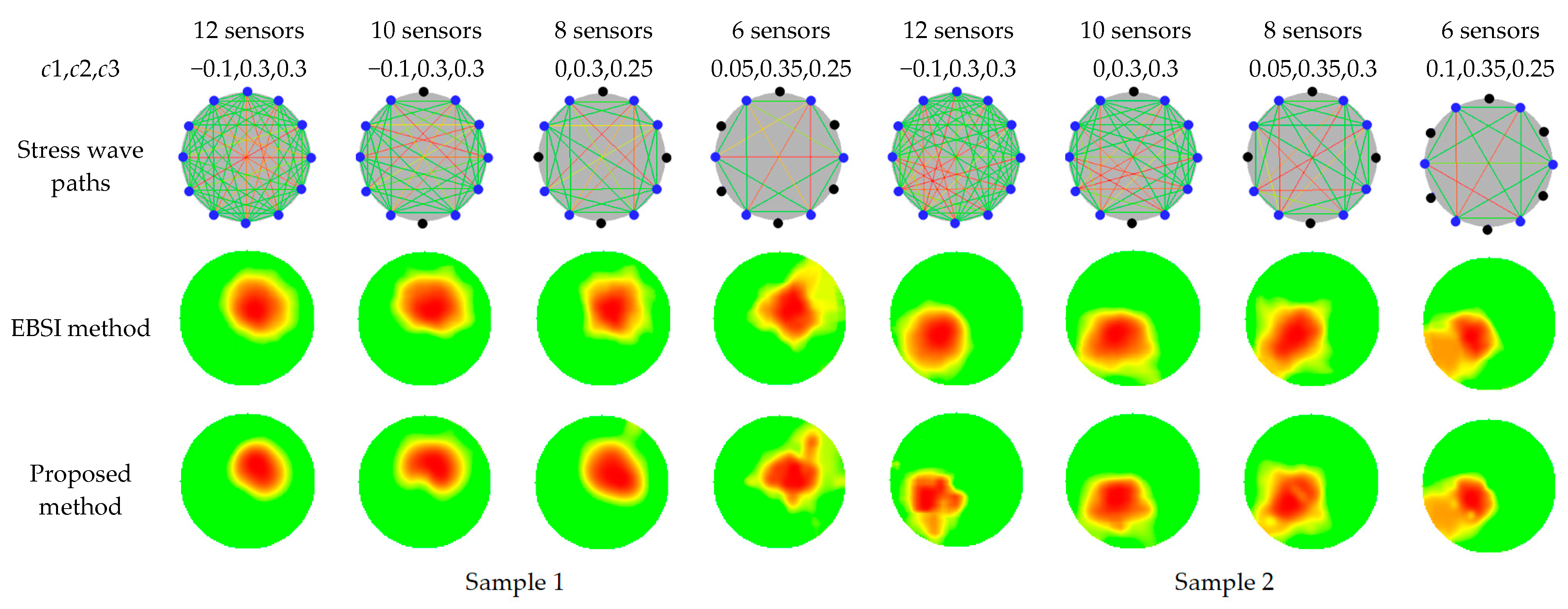
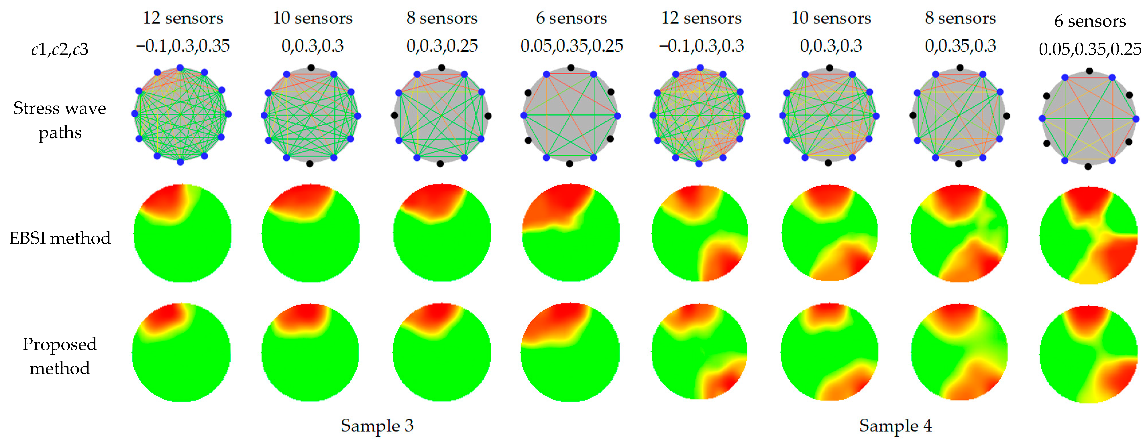
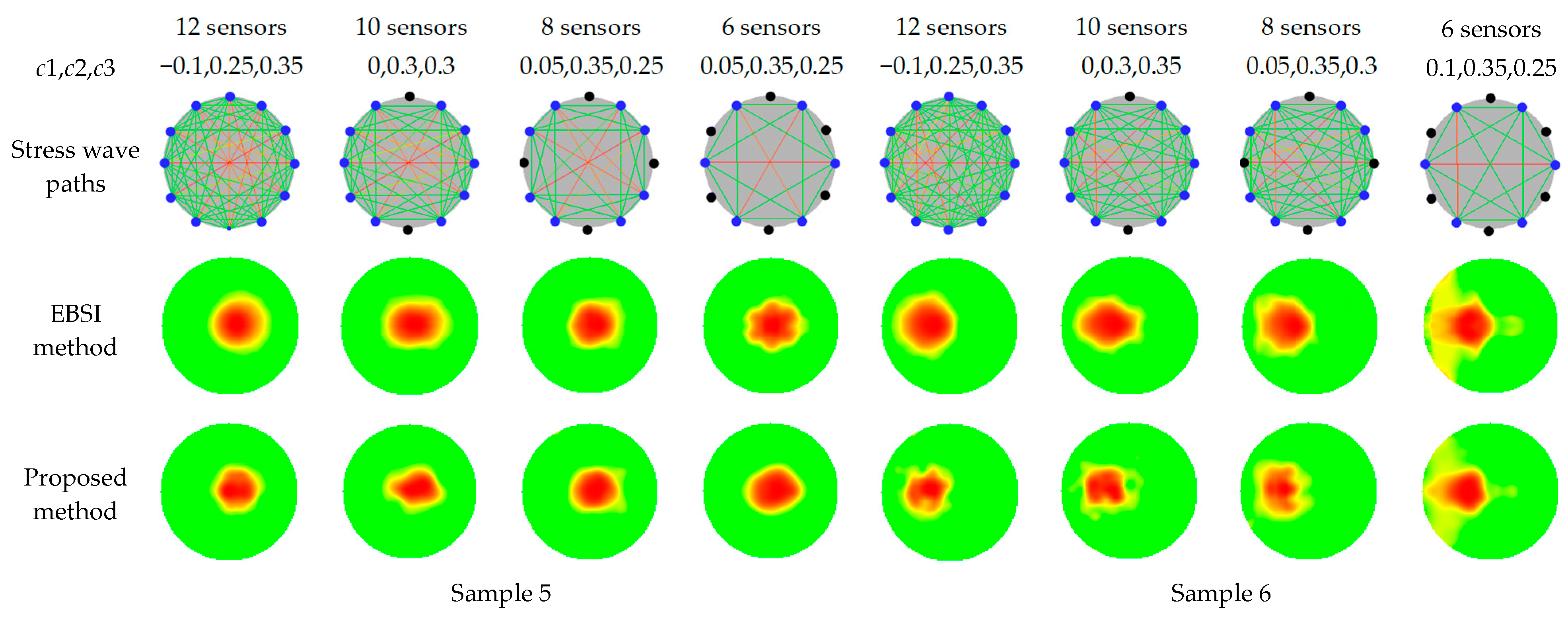
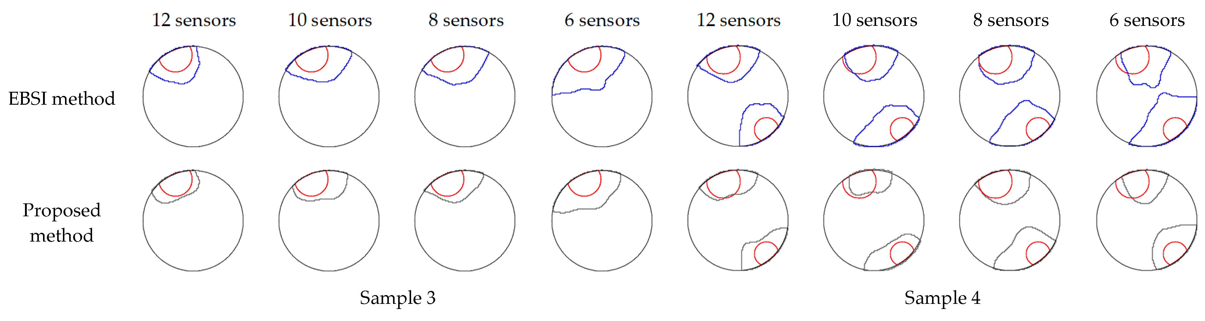
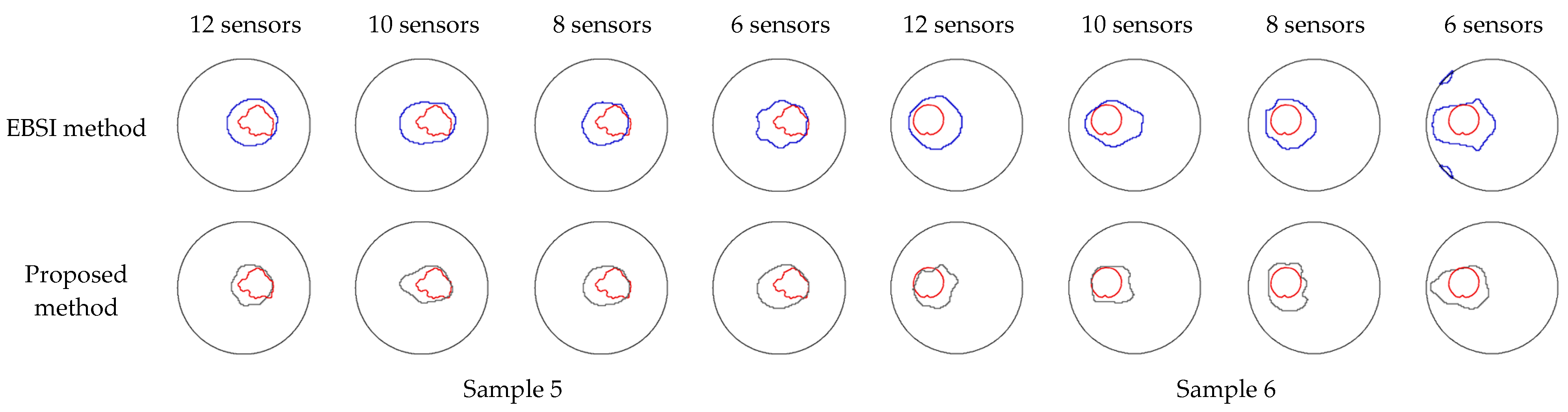
3.1. Imaging Results When the Number of Sensors Decreases

In order to test the imaging performance of the proposed method under sparse signals, for each sample, 12, 10, 8, and 6 sensors are used for imaging experiments, and the sensors are evenly arranged in the cross-section of the tree trunk. The proposed method is also compared with the basic EBSI method to test whether the integration of compressive sensing principles can make the proposed algorithm perform high-quality defect imaging under sparse signals. In addition, c1 is the feature point selection control coefficient in the compressed sensing algorithm result, and c2 and c3 are the feature point selection control coefficients in the EBSI algorithm result. Active sensors are visualized in blue, while unused sensors are visualized in black. The comparative experimental results are shown in Figure 8, Figure 9 and Figure 10.

The comparative experimental results show that both algorithms can achieve relatively good imaging results when the number of sensors is sufficient. However, when the number of sensors decreases, the imaging effects of the two algorithms begin to deteriorate, especially the traditional EBSI algorithm. When the number of sensors decreases to 8 and 6, the imaging results of defects are quite different from the real defects, and some reconstructed defect images even have serious errors such as distortion and adhesion. In contrast, the algorithm proposed in this paper can still ensure a good imaging effect when the number of sensors is reduced to 8 and 6. For all samples, under the condition of the same number of sensors, the imaging results of the proposed algorithm are better than those of the EBSI algorithm in subjective visual perception, which shows that the advantages of the compressed sensing method in sparse representation and solution are helpful for stress wave imaging algorithm to reconstruct high-quality defect images.

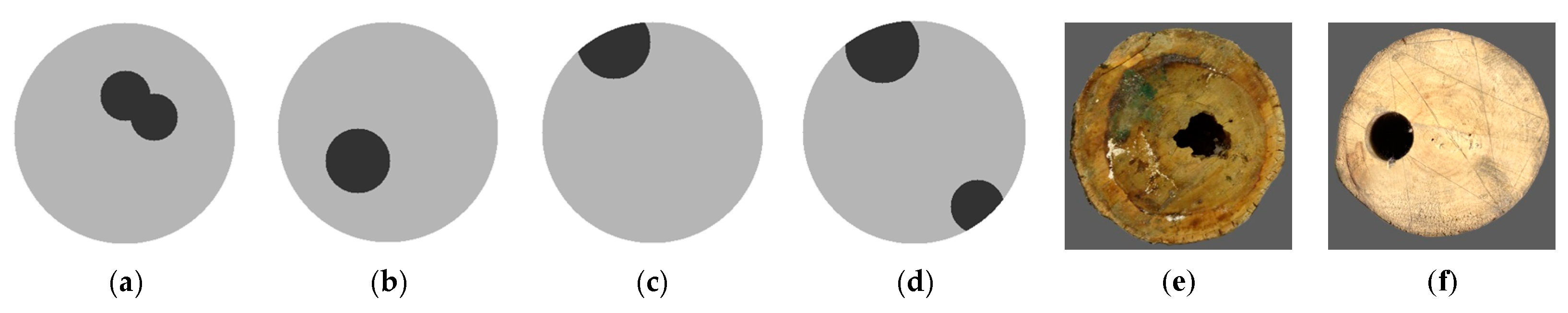
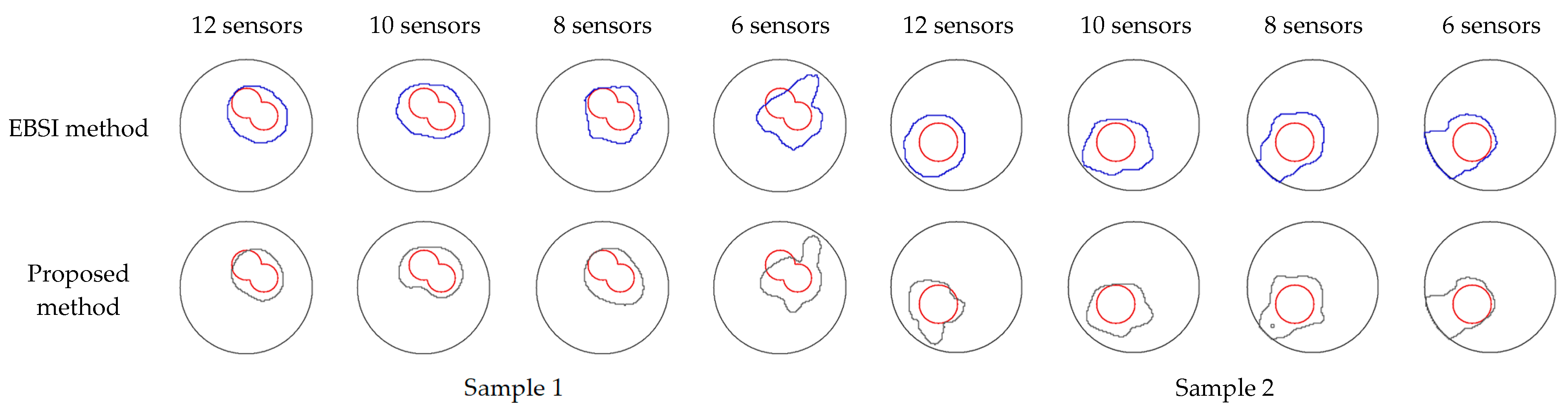
3.2. Defects Area Analysis

In order to quantitatively evaluate the imaging ability of the algorithm proposed in this paper and make a comparative analysis, we use image segmentation technology to obtain the defect regions in all images reconstructed based on EBSI and the proposed method and extract the defect contours. The comparison results of the defect contours are shown in Figure 11, Figure 12 and Figure 13. The red line corresponds to the real contour of the defect, the blue line corresponds to the defect contour extracted from the imaging result of the EBSI algorithm, and the gray line corresponds to the defect contour extracted from the imaging result of the proposed algorithm.

The above comparative experimental results show that the imaging effect of the proposed algorithm is better than that of the EBSI algorithm for all given samples. Especially when the number of sensors is reduced to six, the EBSI imaging results of samples No. 1, No. 2, No. 4, and No. 6 are greatly different from the real defects, which shows that the EBSI method can not guarantee imaging accuracy under sparse signals. The proposed algorithm benefits from the intervention of compressive sensing theory and can maintain a good imaging effect under sparse signals.

The area proportion of actual defects in the cross-section of wood and the comparison results of the area proportion of defects by two imaging methods are shown in Figure 14. Compared with the EBSI method, the experimental results show that the reconstructed defect area of the proposed method is closer to the actual defect area. When the number of sensors decreases, the defect area reconstructed by the proposed algorithm is not much different from the actual defect area. Qualitative imaging results and quantitative defect area proportion prove the effectiveness of the proposed method.

3.3. Defects Shape Analysis

Where the number of sensors decreased from 12 to 6, the accuracy, precision, and recall of the two stress wave imaging algorithms are shown in Figure 15. The comparative experimental results show that as the number of sensors decreases, in most cases, the recall of both algorithms can approach 100%. According to the principle of the confusion matrix, this indicates that the reconstructed defect contours of both algorithms can cover the true defect contours, which is consistent with the research conclusion that spatial interpolation imaging algorithms often overestimate the defect area [32]. Therefore, compared with recall, accuracy and precision can better reflect the performance of the imaging algorithm.

In terms of accuracy, the accuracy of the proposed algorithm is higher than that of the EBSI algorithm for each sample. When the number of sensors is 12, 10, 8, and 6 respectively, the average accuracy of the proposed algorithm is 4.4%, 4.9%, 2.8%, and 4.8% higher than that of the EBSI algorithm. The overall average accuracy of the proposed algorithm is close to 90%, which shows that the algorithm can still maintain high imaging accuracy under sparse signals. In terms of precision, similar to accuracy, the precision of the proposed algorithm is higher than that of the EBSI algorithm for each sample. When the number of sensors is 12, 10, 8, and 6 respectively, the average precision of the proposed algorithm is 11.7%, 10.9%, 5.8%, and 6.1% higher than that of the EBSI algorithm. The precision is lower than the accuracy because the spatial interpolation method overestimates the area of real defects when the input data is insufficient.

3.4. The Visual Impact of Feature Points Extraction on Imaging Results

In order to show the feature points extraction process in detail, and further analyze the contributions of the compressed sensing method and the EBSI method in the proposed algorithm, as well as their collaborative work, we took sample 4 as an example to visualize the detailed process of hybrid imaging.

At first, the impact of c1 on the imaging results was examined. We conducted experiments on all possible values of the control coefficient c1 (i.e., the range from −1 to 1), and in order to clearly display the results, three representative c1 values (min, mid, and max) were selected. When c1 is less than min or greater than max, the corresponding imaging results begin to deteriorate, and mid is the optimal choice for parameter c1.

In order to achieve a relatively balanced number of two types of feature points, a large number of grid points need to be removed from the imaging results of the EBSI algorithm. Therefore, the feature point control parameter c2 = 0.3 is temporarily fixed. In addition, in order to leverage the ability of EBSI to reconstruct healthy areas, the feature points control parameter c3 = 0.25 is temporarily fixed. When there are 12 sensors, the impact of parameter c1 on the imaging process of sample 4 is shown in Figure 16. The first column visualizes the feature points extracted from the compressed sensing imaging results (controlled by parameter c1). The second column visualizes the feature points extracted from the imaging results of the EBSI algorithm (controlled by parameters c2 and c3). The third column shows the visualization results of two types of feature points mixed together. The experimental results show that as the parameter c1 increases, the number of feature points extracted from compressed sensing imaging results continuously increases, and the best hybrid imaging result appears when c1 = −0.1.

Next, we fixed c1 = −0.1 and continued to fix c3 = 0.3 to test the effect of c2 on the imaging results. We conducted experiments on all possible values of the control coefficient c2 (i.e., the range from 0 to 1), and in order to clearly display the results, three representative c2 values (min, mid, and max) were selected. When c2 is less than min or greater than max, the corresponding imaging results begin to deteriorate, and mid is the optimal choice for parameter c2. The impact of parameter c2 on the imaging process of sample 4 is shown in Figure 17. As the parameter c2 increases, the number of feature points extracted from the EBSI algorithm imaging results continues to increase. The imaging results also show that the number of feature points should be appropriate, and the best hybrid imaging result appears at c2 = 0.3.

Finally, we fixed c1 = −0.1 and c2 = 0.3 to test the effect of c3 on the imaging results. We conducted experiments on all possible values of the control coefficient c3 (i.e., the range from 0 to 1). In order to clearly display the results, three representative c3 values (min, mid, and max) were selected. When c3 is less than the min value or greater than the max value, the corresponding imaging results begin to deteriorate, and the mid value is the optimal choice for parameter c3. The impact of parameter c3 on the imaging process of sample 4 is shown in Figure 18. The experimental results show that as parameter c3 increases, the proportion of healthy area feature points in the EBSI algorithm imaging results gradually decreases, and the optimal imaging result appears at c3 = 0.3.

4. Conclusions

A hybrid stress waves imaging method for detecting internal defects in wood under sparse sampling is proposed in this paper. To verify the imaging performance of the proposed method, we used both simulated and real data for defect image reconstruction. Six defect samples with different sizes and positions were tested, and the area and shape of the reconstructed defects were analyzed. In addition, the imaging performance of the algorithm was quantitatively analyzed based on imaging indicators such as accuracy and precision. Based on the experimental results, the following conclusions can be supported:

(1)

With the decrease in the number of sensors and stress wave signals, the imaging effect of the EBSI algorithm and the algorithm proposed in this paper will become worse. However, regardless of the number of sensors, for all samples, compared with the traditional EBSI method, the defect area reconstructed by the proposed method is closer to the actual defect area, and the defect contour reconstructed by the proposed method is also more similar to the actual defect contour.

(2)

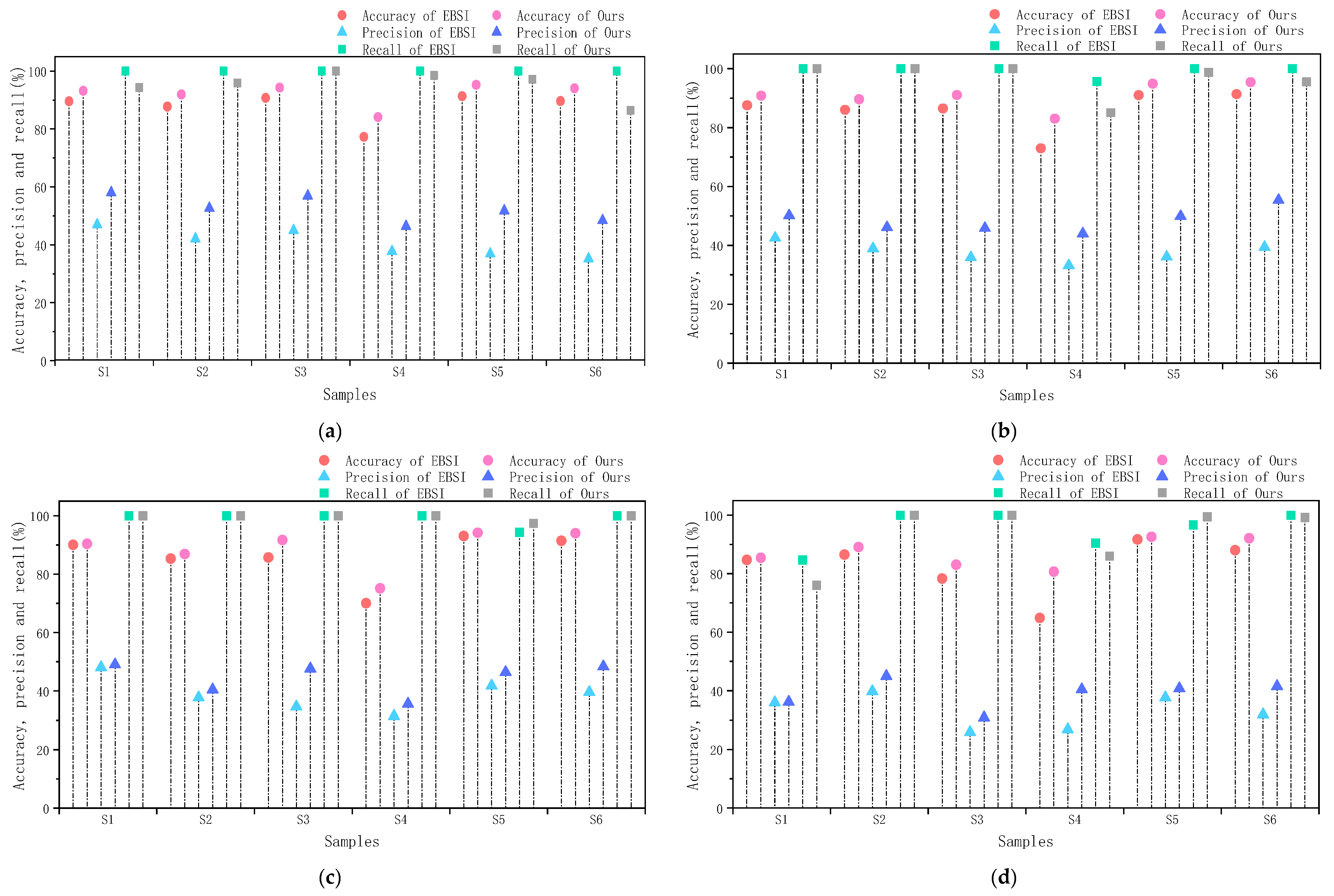
When the number of sensors is 12, 10, 8, and 6, respectively, the average accuracy of the proposed algorithm is 4.4%, 4.9%, 2.8%, and 4.8% higher than that of the EBSI algorithm, and the average accuracy is 11.7%, 10.9%, 5.8%, and 6.1% higher than that of the EBSI algorithm. The overall accuracy of the proposed algorithm reaches 89.7%, while the overall accuracy of the EBSI algorithm is only 85.5%. The ability of the proposed algorithm to resist the reduction of stress wave signals is indicated.

(3)

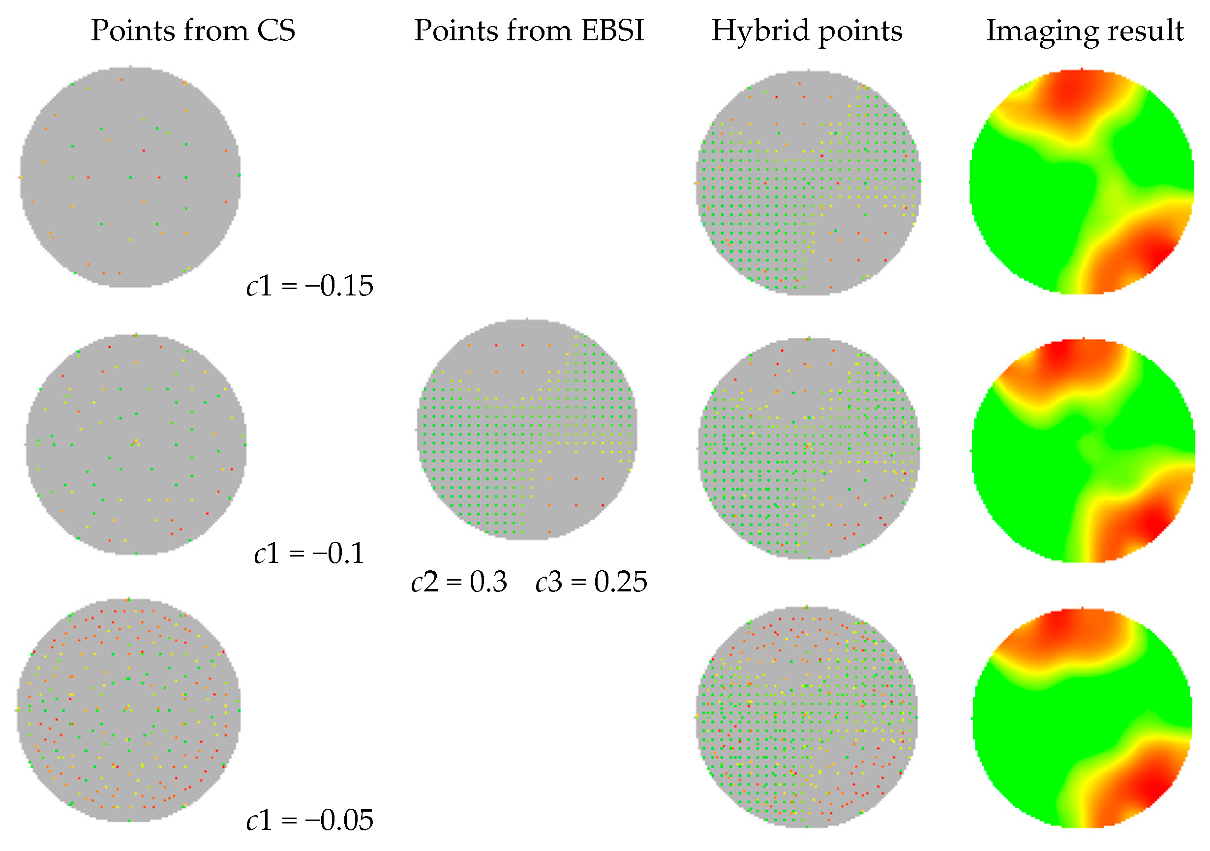
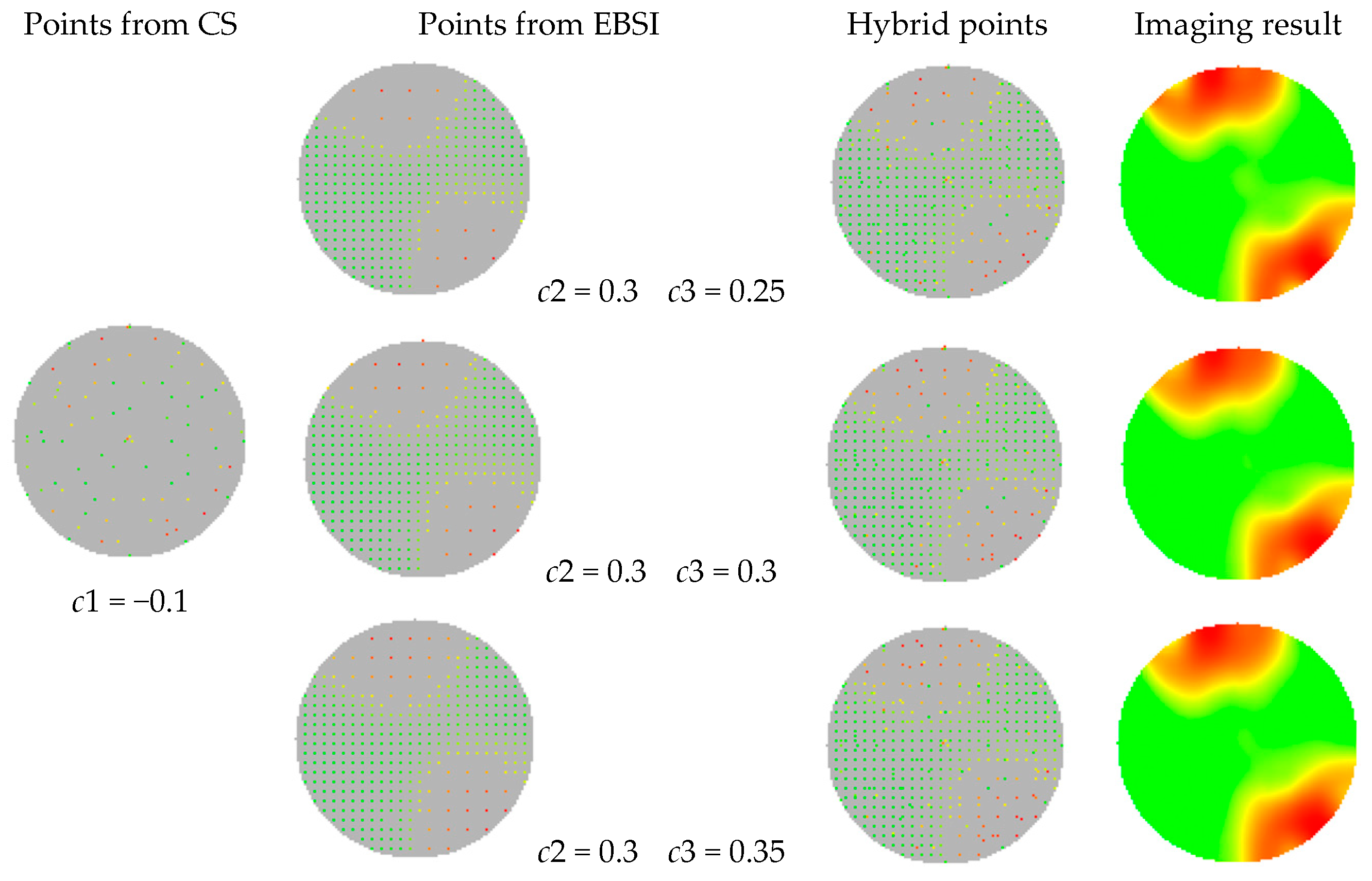
The proper value range of control coefficient c1 is −0.1~0.1. When the number of sensors decreases, c1 gradually increases, indicating that the fewer signals, the higher the participation of the compressive sensing method, which reflects the ability of the theory to reconstruct the velocity distribution in the defect area. The proper value range of control coefficient c2 is 0.25~0.35. When the number of sensors decreases, c2 gradually increases, indicating that the fewer the signals, the higher the participation of the EBSI method. The proper value range of control coefficient c3 is 0.25~0.35. When the number of sensors decreases, c3 gradually decreases, indicating that the fewer the signals, the higher the participation of EBSI in reconstructing healthy areas and the effective boundary suppression of defect areas.

In general, the method proposed in this paper can maintain high imaging accuracy and precision of reconstructed defect images when the number of sensors is reduced. It makes full use of the ability of compressed sensing to recover the defective space area and the ability of the EBSI algorithm to recover the healthy space area, extracts the key feature points from the compressed sensing imaging results and EBSI imaging results, respectively, and completes the hybrid imaging in a unified imaging space. In addition to compressive sensing, other techniques such as deep learning may also be applied to help reconstruct defect images under sparse signals. After designing deep learning models to learn velocity distribution patterns, perhaps in the future, stress wave imaging technology can further reduce the number of sensors.

References

1. Nasir, V.; Ayanleye, S.; Kazemirad, S.; Sassani, F.; Adamopoulos, S. Acoustic emission monitoring of wood materials and timber structures: A critical review. Constr. Build. Mater. 2022, 350, 128877. [Google Scholar] [CrossRef]
2. Simic, K.; Gendvilas, V.; O’reilly, C.; Harte, A.M. Predicting structural timber grade-determining properties using acoustic and density measurements on young sitka spruce trees and logs. Holzforschung 2019, 73, 139–149. [Google Scholar] [CrossRef]
3. Cascón, I.; Sarasua, J.; Tena, M.; Uria, A. Development of an acoustic method for wood disease assessment. Comput. Electron. Agric. 2021, 186, 106195. [Google Scholar] [CrossRef]
4. Rinn, F.; Schweingruber, F.; Schär, E. RESISTOGRAPH and X-ray Density Charts of Wood. Comparative Evaluation of Drill Resistance Profiles and X-ray Density Charts of Different Wood Species. Holzforschung 1996, 50, 303–311. [Google Scholar] [CrossRef]
5. Tannert, T.; Anthony, R.; Kasal, B.; Kloiber, M.; Piazza, M.; Riggio, M.; Rinn, F.; Widmann, R. In Situ Assessment of Structural Timber Using Semi-Destructive Techniques. Mater. Struct. 2013, 47, 767–785. [Google Scholar] [CrossRef]
6. Kobza, M.; Ostrovsk, R.; Adamčíková, K.; Pastirčáková, K. Stability of trees infected by wood decay fungi estimated by acoustic tomography: A field survey. Trees 2021, 36, 103–112. [Google Scholar] [CrossRef]
7. Yang, R.; Xu, Y. Experimental study on dynamic compression behavior characteristics and stress wave propagation law of rigid-flexible combinations under cyclic bi-directional impact loading. J. Mater. Res. Technol. 2023, 25, 925–945. [Google Scholar] [CrossRef]
8. Bandara, S.; Rajeev, P.; Gad, E.; Sriskantharajah, B.; Flatley, I. Structural health assessment of timber utility poles using stress wave propagation and artificial neural network techniques. J. Nondestruct. Eval. 2021, 40, 87. [Google Scholar] [CrossRef]
9. Yang, L.; Dong, X.; Xu, H. Comparison between electrical resistance method and stress wave method in the detection of decay defects in living trees. For. Eng. 2022, 38, 82–88. [Google Scholar]
10. Yamasaki, M.; Tsuzuki, C.; Sasaki, Y.; Onishi, Y. Influence of moisture content on estimating young’s modulus of full-scale timber using stress wave velocity. J. Wood Sci. 2017, 63, 225–235. [Google Scholar] [CrossRef]
11. Van, D.; Dan, R. Estimating mechanical properties of clear wood from ten-year-old melia azedarach trees using the stress wave method. Eur. J. Wood Wood Prod. 2021, 79, 941–949. [Google Scholar]
12. Wessels, C.; Malan, F.; Rypstra, T. A review of measurement methods used on standing trees for the prediction of some mechanical properties of timber. Eur. J. For. Res. 2011, 130, 881–893. [Google Scholar] [CrossRef]
13. Li, L.; Wang, X.; Wang, L.; Allison, R. Acoustic tomography in relation to 2d ultrasonic velocity and hardness mappings. Wood Sci. Technol. 2012, 46, 551–561. [Google Scholar] [CrossRef]
14. Legg, M.; Bradley, S. Measurement of stiffness of standing trees and felled logs using acoustics: A review. J. Acoust. Soc. Am. 2017, 139, 588–604. [Google Scholar] [CrossRef] [PubMed]
15. Yue, X.; Wang, L.; Wacker, J. Electric resistance tomography and stress wave tomography for decay detection in trees—A comparison study. PeerJ 2019, 7, e6444. [Google Scholar] [CrossRef] [PubMed]
16. Rabe, C.; Ferner, D.; Fink, S.; Schwarze, F. Detection of decay in trees with stress waves and interpretation of acoustic tomograms. Arboric. Assoc. J. 2004, 28, 3–19. [Google Scholar] [CrossRef]
17. Arciniegas, A.; Brancheriau, L.; Lasaygues, P. Tomography in standing trees: Revisiting the determination of acoustic wave velocity. Ann. For. Sci. 2015, 72, 685–691. [Google Scholar] [CrossRef]
18. Huan, Z.; Jiao, Z.; Li, G.; Wu, X. Velocity error correction based tomographic imaging for stress wave nondestructive evaluation of wood. BioResources 2018, 13, 2530–2545. [Google Scholar] [CrossRef]
19. Liu, L.; Li, G. Acoustic tomography based on hybrid wave propagation model for tree decay detection. Comput. Electron. Agric. 2018, 151, 276–285. [Google Scholar] [CrossRef]
20. Qiu, Q.; Qin, R.; Lam, J.; Tang, A.; Leung, M.; Lau, D. An innovative tomographic technique integrated with acoustic-laser approach for detecting defects in tree trunk. Comput. Electron. Agric. 2019, 156, 129–137. [Google Scholar] [CrossRef]
21. Du, X.; Li, S.; Li, G.; Feng, H.; Chen, S. Stress Wave Tomography of Wood Internal Defects using Ellipse-Based Spatial Interpolation and Velocity Compensation. Bioresources 2015, 10, 3948–3962. [Google Scholar] [CrossRef]
22. Qin, R.; Qiu, Q.; Lam, J.; Tang, A.; Leung, M.; Lau, D. Health assessment of tree trunk by using acoustic-laser technique and sonic tomography. Wood Sci. Technol. 2018, 52, 1113–1132. [Google Scholar] [CrossRef]
23. Strobel, A.; Renato, J.; Carvalho, G.; Antonio, M.; Goncalves, R. Quantitative image analysis of acoustic tomography in woods. Eur. J. Wood Wood Prod. 2018, 76, 1379–1389. [Google Scholar] [CrossRef]
24. Ross, R.; Brashaw, B.; Pellerin, R. Nondestructive evaluation of wood. For. Prod. J. 1998, 48, 14–19. [Google Scholar]
25. Dackermann, U.; Crews, K.; Kasal, B.; Li, J.; Riggio, M.; Rinn, F.; Tannert, T. In situ assessment of structural timber using stress-wave measurements. Mater. Struct. 2014, 47, 787–803. [Google Scholar] [CrossRef]
26. Chen, L.-C.; Pardeshi, M.S.; Lo, W.-T.; Sheu, R.-K.; Pai, K.-C.; Chen, C.-Y.; Tsai, P.-Y.; Tsai, Y.-T. Edge-glued wooden panel defect detection using deep learning. Wood Sci. Technol. 2022, 56, 477–507. [Google Scholar] [CrossRef]
27. Guo, J.; Wang, P.; Wang, Y.; Xu, H. Improving tree health assessment accuracy at low temperatures: Considering the effect of trunk ice content on electrical resistance and stress wave tomography. J. For. Res. 2023, 34, 1503–1510. [Google Scholar] [CrossRef]
28. Xu, F.; Liu, Y.; Wang, X.; Brashaw, B.K.; Yeary, L.A.; Ross, R.J. Assessing internal soundness of hardwood logs through acoustic impact test and waveform analysis. Wood Sci. Technol. 2019, 53, 1111–1134. [Google Scholar] [CrossRef]
29. Du, X.; Li, J.; Feng, H.; Chen, S. Image reconstruction of internal defects in wood based on segmented propagation rays of stress waves. Appl. Sci. 2018, 8, 1778. [Google Scholar] [CrossRef]
30. Zheng, Q.; Zhao, W.; Xu, F.; Liu, Y. Wood stresswave nondestructive testing tomography algorithm based on asymmetric ellipse. J. For. Eng. 2023, 8, 137–143. [Google Scholar]
31. Liu, T.; Li, G. Stress wave tomography imaging algorithm based on ray segmentation for nondestructive testing of Wood. Sci. Silvae Sin. 2021, 57, 181–192. [Google Scholar]
32. Liang, S.; Fu, F. Effect of sensor number and distribution on accuracy rate of wood defect detection with stress wave tomography. Wood Res. 2014, 59, 521–531. [Google Scholar]
33. Giryes, R.; Eldar, Y.; Bronstein, A.; Sapiro, G. Tradeoffs between convergence speed and reconstruction accuracy in inverse problems. IEEE Trans. Signal Process. 2018, 66, 1676–1690. [Google Scholar] [CrossRef]
34. Wang, X. Acoustic measurements on trees and logs: A review and analysis. Wood Fiber Sci. 2013, 47, 965–975. [Google Scholar] [CrossRef]
35. Fang, Y.; Feng, H.; Li, J.; Li, G. Stress wave signal denoising using ensemble empirical mode decomposition and an instantaneous half period model. Sensors 2011, 11, 7554–7567. [Google Scholar] [CrossRef]
36. Donoho, L. Compressed sensing. IEEE Trans. Inf. Theory 2006, 52, 1289–1306. [Google Scholar] [CrossRef]
37. Chartrand, R.; Staneva, V. Restricted isometry properties and nonconvex compressive sensing. Inverse Probl. 2010, 24, 657–682. [Google Scholar]
38. Ji, S.; Dunson, D.; Carin, L. Multitask Compressive Sensing. IEEE Trans. Signal Process. 2009, 57, 92–106. [Google Scholar] [CrossRef]
39. Yoon, H.; Kim, K.; Kim, D. Motion Adaptive Patch-Based Low-Rank Approach for Compressed Sensing Cardiac Cine MRI. IEEE Trans. Med. Imaging 2014, 33, 2069–2085. [Google Scholar] [CrossRef]
40. Valiollahzadeh, S.; Clark, J.; Mawlawi, O. MO-D-141-05: Dictionary Learning in Compressed Sensing Using Undersampled Data in PET Imaging. Med. Phys. 2013, 40, 400. [Google Scholar] [CrossRef]
41. Liu, J.; Lian, F.; Mallick, M. Distributed compressed sensing based joint detection and tracking for multistatic radar system. Inf. Sci. 2016, 369, 100–118. [Google Scholar] [CrossRef]
42. Wu, X.; Huang, G.; Wang, J. Image reconstruction method of electrical capacitance tomography based on compressed sensing principle. Meas. Sci. Technol. 2013, 24, 075401. [Google Scholar] [CrossRef]
43. Zhang, W.; Tan, C.; Xu, Y. Electrical Resistance Tomography Image Reconstruction Based on Modified OMP Algorithm. IEEE Sens. J. 2019, 19, 5723–5731. [Google Scholar] [CrossRef]
44. Hettler, J.; Tabatabaeipour, M.; Delrue, S.; Van, D. Linear and nonlinear guided wave imaging of impact damage in cfrp using a probabilistic approach. Materials 2016, 9, 901. [Google Scholar] [CrossRef]
45. Xu, L.; Lu, C.; Zhou, T.; Wu, J.; Feng, H. A 3D-2DCNN-CA approach for enhanced classification of hickory tree species using UAV-based hyperspectral imaging. Microchem. J. 2024, 199, 109981. [Google Scholar] [CrossRef]
Figure 1. Illustration of traditional stress wave imaging: (a) visualization of propagation paths; (b) traditional EBSI algorithm; (c) imaging area.
Forests 15 01139 g001
Figure 2. Self-developed apparatus: (a) signal processing box; (b) toolbox; (c) sensor (angle 1); (d) sensor (angle 2); (e) self-developed software (interface 1); (f) self-developed software (interface 2).
Forests 15 01139 g002
Figure 3. Acquisition of stress wave signals.
Forests 15 01139 g003
Figure 4. Simulation samples and tree trunks: (a) overlapping double circle; (b) single circle distribution; (c) edge semi-circle; (d) double edge semi-circle; (e) Pecan tree trunk with cavity; (f) Camphor tree trunk with cavity.
Forests 15 01139 g004
Figure 5. Illustration of proposed stress wave hybrid imaging for detecting wood internal defects.
Forests 15 01139 g005
Figure 6. Illustration of feature point extraction strategy in compressed sensing imaging results: (a) feature point deletion strategy; (b) feature point supplement strategy.
Forests 15 01139 g006
Figure 7. Visualization of the confusion matrix.
Forests 15 01139 g007
Figure 8. Comparative imaging results of samples 1 and 2 with decreasing number of sensors.
Forests 15 01139 g008
Figure 9. Comparative imaging results of samples 3 and 4 with decreasing number of sensors.
Forests 15 01139 g009
Figure 10. Comparative imaging results of samples 5 and 6 with decreasing number of sensors.
Forests 15 01139 g010
Figure 11. Comparative defect contours of samples 1 and 2.
Forests 15 01139 g011
Figure 12. Comparative defect contours of samples 3 and 4.
Forests 15 01139 g012
Figure 13. Comparative defect contours of samples 5 and 6.
Forests 15 01139 g013
Figure 14. Comparison of area proportion of reconstructed defects with different numbers of sensors: (a) 12 sensors; (b) 10 sensors; (c) 8 sensors; (d) 6 sensors.
Forests 15 01139 g014
Figure 15. Comparison of accuracy, precision, and recall with different numbers of sensors: (a) 12 sensors; (b) 10 sensors; (c) 8 sensors; (d) 6 sensors.
Forests 15 01139 g015
Figure 16. The impact of parameter c1 on the imaging process of sample 4 with 12 sensors.
Forests 15 01139 g016
Figure 17. The impact of parameter c2 on the imaging process of sample 4 with 12 sensors.
Forests 15 01139 g017
Figure 18. The impact of parameter c3 on the imaging process of sample 4 with 12 sensors.
Forests 15 01139 g018
Disclaimer/Publisher’s Note: The statements, opinions and data contained in all publications are solely those of the individual author(s) and contributor(s) and not of MDPI and/or the editor(s). MDPI and/or the editor(s) disclaim responsibility for any injury to people or property resulting from any ideas, methods, instructions or products referred to in the content.