Spatiotemporal Changes in Ecological Quality and Its Response to Forest Landscape Connectivity—A Study from the Perspective of Landscape Structural and Functional Connectivity

Abstract

Understanding the response of ecological quality (EQ) to forest landscape connectivity is essential to global biodiversity conservation and national ecological security. However, quantitatively measuring the properties and intensities within these relationships from a spatial heterogeneity perspective remains challenging. This study takes the Fujian Delta region as its case study. The Google Earth Engine platform was employed to compute the remote sensing ecological index (RSEI), the landscape metrics were applied to represent the structural connectivity of the forest landscape, and the minimum cumulative resistance model was adopted to measure the cost distance index representing the functional connectivity of the forest landscape. Then, the spatial correlation and heterogeneity between the EQ and forest landscape connectivity were analyzed based on spatial autocorrelation and geographical weighted regression at three scales (3, 4, and 5 km). The results showed the following: (1) from 2000 to 2020, the overall EQ increased, improving in 37.5% of the region and deteriorating in 13.8% of the region; (2) the forest landscape structural and functional connectivity showed a small decreasing trend from 2000 to 2020, decreasing by 1.3% and 0.9%, respectively; (3) eight forest landscape structural and functional connectivity change modes were detected under the conditions of an improving or degrading EQ based on the change in RSEI and forest landscape structural and functional connectivity; (4) the geographical weighted regression results showed that compared with the forest landscape structural connectivity index, the cost distance index had the highest explanatory power to RSEI in different scales. The effect of forest landscape functional connectivity on EQ is greater than that of structural connectivity. It provides a scientific reference for ecological environmental monitoring and the ecological conservation decision-making of managers.

1. Introduction

Forests play an important role in soil conservation, carbon sequestration, climate regulation, and biodiversity protection [1]. However, the encroachments on forest land caused by logging and rapid urban expansion have led to large areas of forests becoming fragmented into isolated patches [2,3], triggering severe forest landscape fragmentation [4], reducing forest landscape connectivity [5], and ultimately leading to widespread ecological problems such as ecological degradation and the loss of global biodiversity [6,7]. Forest landscape connectivity is closely related to ecosystem integrity, stability, and sustainability [8]. Maintaining high landscape connectivity is an important component in the sustainable planning and management of forest landscapes. Therefore, we need to analyze the relationship between ecological quality (EQ) and forest landscape connectivity in the context of the significant phenomenon of widespread forest landscape fragmentation. Exploring this response can assist in mitigating the adverse effects of global climate change, protecting biodiversity, and ensuring ecological security.

Ecological quality is defined as the degree to which the ecological environment is good or bad. Based on the theory of ecology, it reflects the suitability of the ecological environment for human survival and sustainable socio-economic development within a specific time and space, and at the level of the ecosystem [9]. Many studies have been conducted on the effects of forest landscape patterns on the environment [10,11]. For example, Peng et al. [12] found that the complexity of woodland shapes and the dispersion of each woodland had a significant cooling effect on regional temperatures. Crompton et al. [13] found that deforestation leads to higher surface temperatures and that surface warming from deforestation is impacted by forest fragmentation. Li et al. [14] found that the edge effect significantly affected soil moisture, soil temperature, and air temperature 15 m inward from the forest boundary. However, there are some shortcomings in the present research. Traditional remote sensing surveillance methods are mostly evaluated based on a single index [15], such as the normalized differential vegetation index (NDVI) [16], a permanent vegetation coverage rate [17], land surface temperature (LST) [18], and a standardized precipitation index [19]. However, such individual indicators can only unilaterally explain one aspect of the ecological situation and cannot fully capture the complexity of the environment [20]. Subsequently, some comprehensive evaluation indicators have been developed, for instance, the pressure–state–response model [21] and the ecological index [22]. However, there are limitations to these indicators in terms of the difficulty in obtaining data as well as a lack of objectivity in the weight calculations [23]. Xu [24] constructed a remote sensing-based ecological index (RSEI), founded on remote sensing technology via the integration of the four indicators of greenness, heat, dryness, and wetness using principal component analysis (PCA) [25]. An RSEI has many advantages such as visualization and has been widely used [26,27]. However, the selection of RSEI metrics involves different satellite products and generates a large amount of data, making data preprocessing cumbersome [28]. The advent of the Google Earth engine (GEE) has provided a new perspective on the rapid calculation of the RSEI [29,30]. In addition, conventional landscape indices, such as edge density and patch density (PD), were used for forest landscape pattern metrics [31], none of which considered the effect of the landscape matrix on landscape connectivity. Because landscape connectivity depends on the observation scale [32], the relationship between landscape connectivity and EQ is also scale-dependent. Therefore, it is crucial to consider the influence of scale effects when assessing the impact of forest landscape patterns on EQ.

Landscape connectivity can be defined as the degree to which the landscape either facilitates or impedes the movement of organisms or changes in some ecological process between source patches; it includes the concepts of structural and functional connectivity [33]. Landscape structural connectivity refers to the degree of continuity between the spatial structural units of the landscape [34]. The functional connectivity of the landscape is determined by the interaction of the landscape’s structural continuity and species migration [35]. Traditional landscape connectivity studies have focused on landscape structural connectivity without considering the impedances of animal passage [36], such as those based on the characterization of landscape pattern indices [37]. In recent years, various methods have been developed to measure the degree of functional connectivity of landscapes, such as the minimum cumulative resistance model (MCR) [38,39], the graph theory method [40], and the current theory method [41,42]. Among these approaches, the MCR model, which can be calculated based on organisms’ resistance coefficients as they pass through different landscape units, is itself a measure of functional connectivity and is widely used [43]. For example, based on the principles of the MCR model, Belote et al. [41] comparatively identified significant areas of landscape connectivity in North America by establishing different modeling scenarios. Gonzalez et al. [44] evaluated the landscape functional connectivity of fire propagation based on the MCR model. Therefore, the construction of a cost distance index (CD) has proved to be reliable in quantifying the functional connectivity of landscapes based on the MCR model. In addition, the comprehensive assessment of the forest landscape’s structural and functional connectivity has become increasingly complex because rapid urbanization is causing dramatic changes in land use, while both afforestation and deforestation are dynamic processes. The connectivity of forested landscapes is often considered to be related to EQ. However, forest landscape connectivity and EQ do not always go hand in hand. If EQ or forest landscape connectivity are considered separately, the reliability of the estimation of dynamic change in the forest landscape pattern will be reduced. Therefore, an urgent need exists to comprehensively analyze the changes in EQ as well as the landscape structural and functional connectivity patterns of forests in order to provide references for the scientific management decisions related to forest landscapes.

Currently, most of the methods concerning the response of the environment to forest landscape patterns are based on global regression, such as regression analysis [12], correlation analysis [45,46], and ordinary least squares (OLS) [47] regression. However, these methods assume a level of homogeneity in the relationships between the variables, i.e., they generate global relationships that reflect only the average conditions. Some locally specific relationships may remain hidden [48]; the relationships being concealed renders them inadequate for analyzing spatial data with spatial autocorrelation and heterogeneity, and prone to scale mismatch errors and overfitting [49]. Furthermore, the uneven spatial distribution of natural and ecological resources, such as forests, often leads to the presence of spatial heterogeneity and autocorrelation. This makes it difficult for traditional global regression methods to consider the differences caused by the influence of spatial changes in factors influencing RSEI from the perspective of spatial heterogeneity [50]. Given the obvious ecological differences between forested areas and construction land located in the Fujian Delta region, it is essential to investigate the relationship between RSEI and forest landscape connectivity in terms of spatial heterogeneity when assessing EQ drivers [51]. Geographically weighted regression (GWR) is mainly used to solve the spatial heterogeneity problem [52,53]. This model integrates the ideas of both variable parameters and local regression. The regression coefficients of each sample point can be obtained, so as to differentiate the local spatial characteristics of the relationships between the variables and realize the precise geographic identification of the heterogeneity of a spatial relationship.

As the core area of the national ecological civilization pilot zone (Fujian), the forest landscape features in the Fujian Delta region are typical. Due to the rapid development of urbanization, forest changes are more active, which leads to landscape fragmentation and ecological risks, causing many ecological problems such as geological disasters [54]. As a result, the Fujian Delta region has long been facing the pressure of a difficult coordination between ecological protection and economic development. Therefore, this study takes the Fujian Delta area as its study area. In the present study, RSEI was calculated based on the GEE platform to evaluate the EQ of the Fujian Delta region. Spatial autocorrelation and multiscale hotspots were used to analyze the spatial differentiation characteristics of the RSEI. The landscape metrics were applied to represent the structural connectivity of the forest landscape, and the minimum cumulative resistance model was adopted to measure the cost distance index representing the functional connectivity of the forest landscape. The spatial correlation and heterogeneity of EQ and the forest landscape structural and functional connectivity were analyzed at different scales based on spatial autocorrelation and GWR. Therefore, this study aimed to (1) assess and visualize spatiotemporal patterns of EQ in the Fujian Delta region from 2000 to 2020; (2) identify spatially differentiated features of EQ; (3) analyze spatiotemporal changes in forest landscape structural and functional connectivity from 2000 to 2020; and (4) determine the relationship between forest landscape structural and functional connectivity and EQ at different scales. This study aims to answer the following two questions: (1) what is the change in EQ in the Fujian Delta region from 2000 to 2020? and (2) what is the response relationship of EQ to the forest landscape structural and functional connectivity? The study’s findings can serve as a reference point for formulating rational regional planning and conservation strategies.

2. Materials and Methods

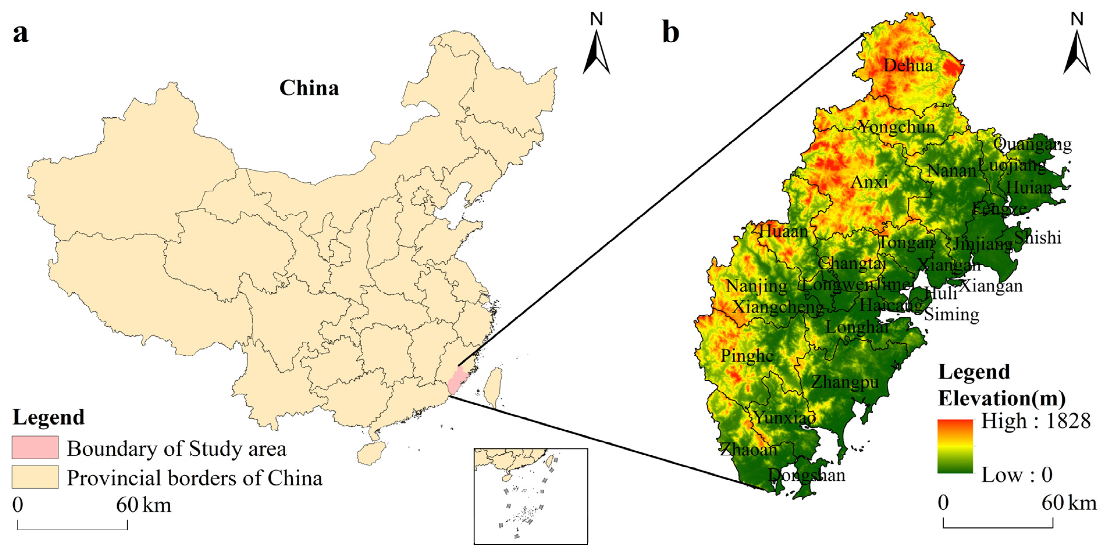
2.1. Study Area

The Fujian Delta region (116°53′21″ E–119°01′38″ E, 23°33′20″ N–25°56′45″ N) is located along the southeastern coast of China’s Fujian Province, across the sea from Taiwan, and includes the cities of Zhangzhou, Quanzhou, and Xiamen, covering a total area of approximately 25,000 km² (Figure 1). The Fujian Delta region has typically subtropical maritime monsoon weather, with average annual temperatures stabilizing between 20.8 and 23.6 °C and a mean rainfall of 1400–2000 mm. However, as one of the important nodes of the Maritime Silk Road, the Fujian Delta region has a population of more than 18.31 million [55], according to the statistical yearbook of 2022. The Fujian Delta has experienced rapid urbanization [56], with the urbanization rate rising from 40.3% to 69.37% in the period from 2000 to 2020 [57]. Ecological land, such as forests, is occupied by construction land, and the landscape pattern is changing dramatically, which leads to the intensification of landscape ecological risks. The balance between economic development and ecological protection is under significant pressure. Moreover, the forest landscape coverage rate of the Fujian Delta region is close to 50%, with typical forest landscape characteristics, and mountains and hills accounting for more than 80% of the area. The complex natural conditions lead to a fragile ecosystem, which facilitates the occurrence of natural disasters, and thus destroys the original EQ [54]. There are significant challenges inherent in the construction of an ecological civilization. Therefore, the study of the spatiotemporal changes in the EQ and its response to forest landscape structural and functional connectivity in the Fujian Delta region has extensive research value. The results can provide a scientific reference for the sustainable development of other similar cities.

2.2. Methodology

2.2.1. Data Sources and Preprocessing

Landsat TM/OLI/TIRS remote sensing image data with a spatial resolution of 30 m were downloaded using the GEE platform [58]. The Landsat series images were preprocessed with geometric accuracy correction, radiometric correction, and atmospheric correction [59]. In order to minimize the effect of seasonal fluctuations, remote sensing images from the summer (May to September) of the target year and the years before and after were selected, and the images were synthesized using the median synthesis method. An officially provided cloud masking method was used to remove the cloud layer to meet the required accuracy for this study [60]. In addition, because the wetness component was principally closely related to the vegetation and soil moisture, in order to reduce the impact of water bodies, which account for 3.09% of the area of the Fujian Delta, the modified normalized difference water index was used to mask the water body and ensure the reliability of the analyses performed [24].

Other data used in the study consisted primarily of land use data, road network data, and digital elevation model (DEM) data. Among them, the 30 m resolution land use data were obtained from the Resource and Environment Science Data Center of the Chinese Academy of Sciences (http://www.resdc.cn, accessed on 16 April 2023). Road network data were obtained from the OpenStreetMap website (http://www.openstreetmap.org, accessed on 12 May 2023). The DEM data were obtained from the Geospatial Data Cloud Platform of the Computer Network Information Center of the Chinese Academy of Sciences (http://www.gscloud.cn, accessed on 25 May 2023). Slope data were created from DEM data. All data were normalized for comparability. To ensure the reliability of the results, data with a spatial resolution of 30 m were used [57]. All of the above data were converted to the krasovsky_1940_Albers projected coordinate system using ArcGIS 10.7 software.

2.2.2. Calculation of RSEI

The four indicator components of RSEI were obtained entirely based on remote sensing image extraction [24,61]. The four metrics coupled to RSEI were those of NDVI; LST; wetness (WET), which was obtained through tassel cap transformation; and dryness, represented by the normalized difference built-up index and soil index (NDBSI). Then, the weights of the components were determined objectively using PCA, avoiding the subjectivity of artificially determined weights. The detailed formulas for the RSEI and the components are provided in Supplementary Materials (Appendix S1). In order to analyze the changes in EQ, the RSEI equal intervals were classified into five categories, from low to high, as poor (0–0.2), fair (0–0.2), moderate (0.2–0.4), good (0.6–0.8), and excellent (0.8–1) [62].

2.2.3. Hot Spot Analysis

As a method to explore the characteristics of local spatial clustering distributions, hotspot analysis can be used to analyze how high or low values of RSEI are spatially clustered [63]. Since RSEI at the various scales have different spatial differentiation characteristics, grid scales (1, 2, 3, 4, and 5 km) and county scales were set. The calculations were performed using the Hot Spot Analysis tool in ArcGIS 10.7, and its detailed formulas are shown in Supplementary Materials (Appendix S2).

2.2.4. Calculation of Structural Connectivity Indices for Forest Landscapes

Landscape indices are quantitative metrics that describe information about various aspects of the landscape pattern, reflecting its composition and configuration [29]. Twelve commonly used landscape indices were selected at the class level, referring to previously conducted studies [64,65]. Because redundant indicators have the same meaning in the landscape index, in order to reduce redundancy, only feature category information was retained in this research. The following four landscape indices were selected through correlation analysis [66,67]: PD, the largest patch index (LPI), the aggregation index (AI), and the patch cohesion index (COHESION). These indices were calculated using the square moving window (1200 m × 1200 m) method in the Fragstats 4.2 software. Then, the results were normalized (Appendix S3).

Based on the above four landscape indices, the forest landscape structural connectivity composite index (FLSCC) was constructed using PCA [5]. The contribution rate of the first principal component (PC1) was greater than 83%, indicating that PC1 had integrated most of the characteristic information of all indicators (Appendix S4). Therefore, PC1 was proposed for the construction of the FLSCC.

2.2.5. Calculation of Functional Connectivity Index of Forest Landscapes

A CD was constructed based on the MCR model to characterize the degree of landscape functional connectivity. First, four resistance factors, namely land use type, slope, distances to construction land, and roads, were selected to construct a single-factor resistance surface [68]. The higher the resistance value, the more difficult it is for a species to overcome the resistance to achieve migration from the source to the destination sites [69]. In reference to the previously obtained findings in studies, the resistance size of different landscape types in the region was set as one for forest, five for grassland, eight for cropland, nine for unused land, and ten for construction land and water. The construction land resistance values varied depending on the distance between the construction land and the source site. The distance from the construction land had resistance values of one for >2000 m, seven for 1500–2000 m, eight for 1000–1500 m, nine for 500–1000 m, and ten for <500 m. The magnitude of the road resistance values likewise varied with distance from the nearest roadway. The resistance values were one for a distance >1500 m from the road, seven for 1000–1500 m, eight for 500–1000 m, nine for 100–500 m, and ten for <100 m. Considering the effects of slope, the resistance values were set to one, seven, eight, nine, and ten for areas with slopes of 0–5°, 5–15°, 15–25°, 25–35°, and >35°, respectively. Second, factor analysis was used to calculate the weights of individual resistance factors. The four one–factor resistance surfaces were then superimposed using a raster calculator to form a composite resistance surface for analysis. Finally, based on ArcGIS 10.7, a CD was calculated through the combination of the integrated resistance surface [70,71] with the forest as the source. Then, the results were normalized. The CD was calculated as follows:

$$CD=f_{min}{\sum }_{j=n}^{i=m}(D_{ij}\times R_i)$$

(1)

where CD is the minimum cumulative resistance value; f is a positive function between CD and the variable ($D_{ij}$ × $R_i$); $D_{ij}$ is the spatial distance from the diffusion of source j to the spatial cell i; and $R_i$ is the resistance coefficient of the spatial cell i.

2.2.6. Spatial Autocorrelation Analysis

Spatial autocorrelation reflects the degree of similarity of attribute values of spatially neighboring regional units, including global Moran’s I and local indicators of spatial association (LISA). This method can analyze single or multiple variables [72], and the detailed calculations for Moran’s I are provided in Appendix S5.

Because spatial autocorrelation analysis in a single region is highly susceptible to scale effects, the county scale and five different scales of fishing nets (1, 2, 3, 4, and 5 km) were created as the spatial units of analysis.

For the study of the forest landscape connectivity index (PD, LPI, AI, COHESION, FLSCC, and CD) and spatial correlation of RSEI, bivariate spatial autocorrelation was chosen [73]. In order to study the relationship between the two at different scales, the fishing nets (1, 2, 3, 4, and 5 km) were created as spatial units of analysis.

2.2.7. Geographically Weighted Regression Model

The GWR model was used to analyze the effects of forest landscape structural and functional connectivity on EQ. Compared with the OLS model, the GWR model overcomes the non-stationarity and dependence of the spatial data [74]. GWR was calculated using the following methodology:

$$y_i={\beta }_0\left(u_i,v_i\right)+\sum _{i=1}^n{\beta }_k\left(u_i,v_i\right)x_{ik}+{\epsilon }_i$$

(2)

where $y_i$ is the RSEI value of the ith cell, ($u_i,v_i$) is the center geographic coordinate of the ith cell, ${\beta }_0\left(u_i,v_i\right)$ is the intercept term, ${\beta }_k\left(u_i,v_i\right)$ is the regression coefficient of the ith cell, and ${\epsilon }_i$ is the random error term.

In the determination of the spatial weight matrix, a Gaussian function was chosen as the spatial weight function. The Akaike information criterion (AIC) method was used to determine the optimal bandwidth and compare the significance of different models. When the difference between the AIC values of the two models was greater than three, the model with the smallest AIC value had a better simulation effect [75].

3. Results

3.1. Spatiotemporal Dynamics in EQ

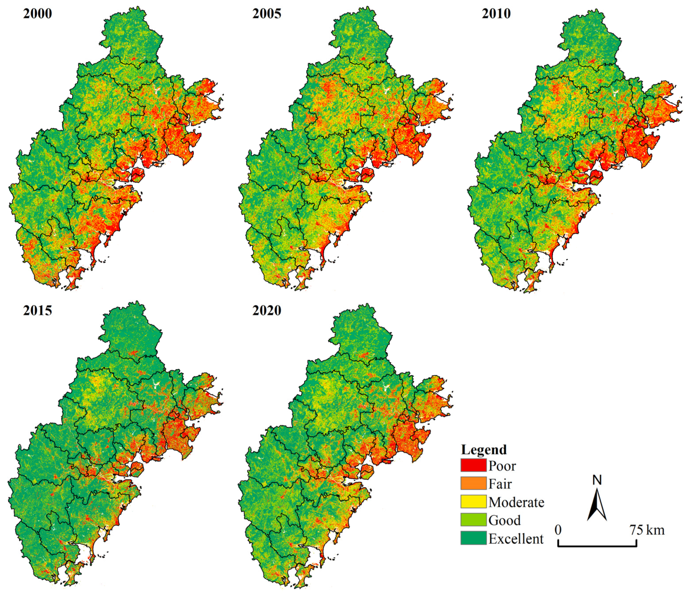
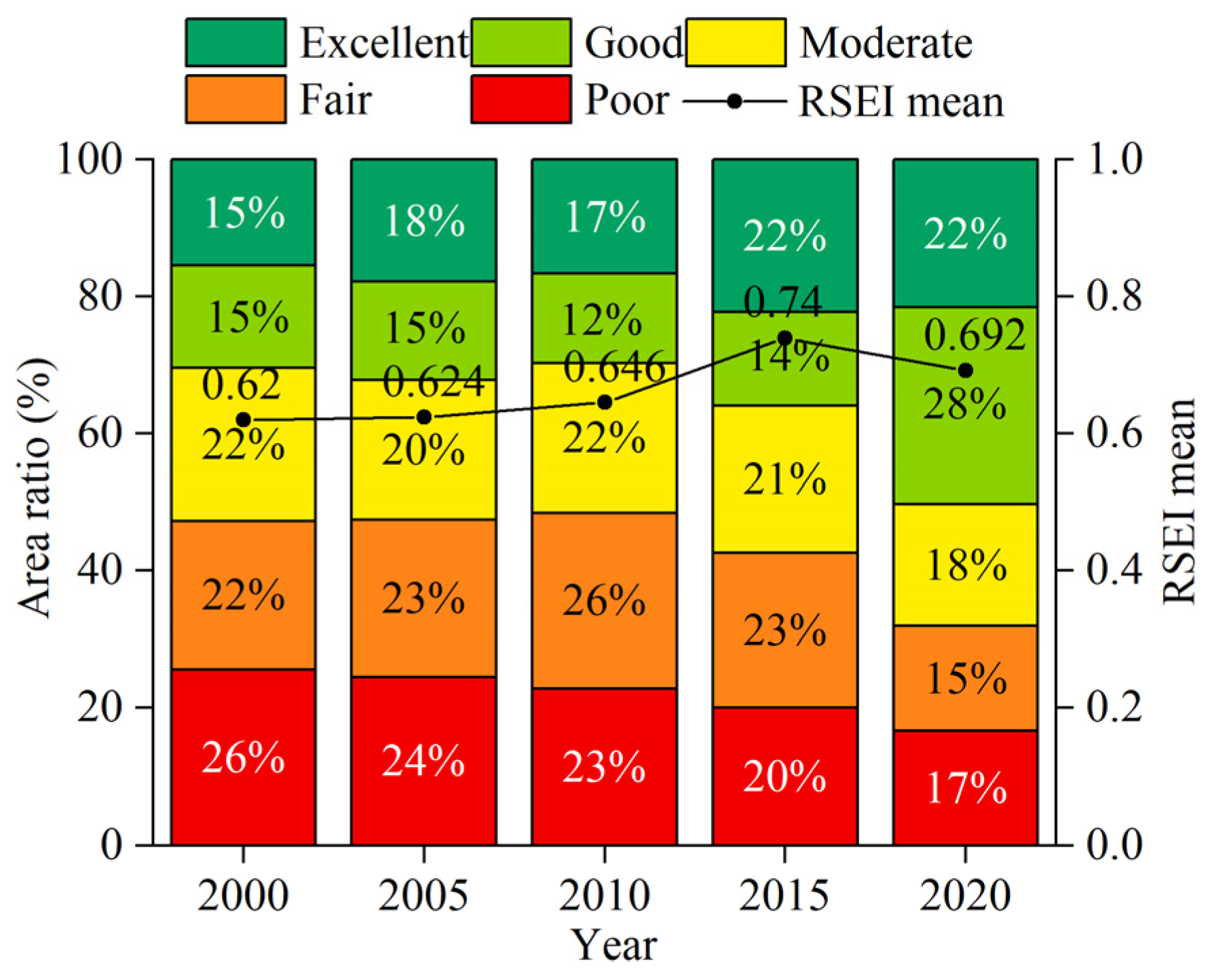
3.1.1. The State of EQ in Fujian Delta Region

The contribution of the PC1 was more than 81% in all years (

Table 1. Principal component analysis of four component indices.

Year		NDVI	WET	LST	NDBSI	Eigenvalue	Percentage Eigenvalue (%)
2000	PC1	0.455	0.457	−0.587	−0.489	0.291	81.29
	PC2	−0.265	0.686	0.597	−0.321	0.039	10.98
	PC3	0.711	−0.336	0.540	−0.300	0.024	6.67
	PC4	–0.466	–0.455	–0.088	–0.754	0.004	1.06
2005	PC1	0.508	0.480	−0.461	−0.547	0.251	83.97
	PC2	0.513	−0.715	−0.427	0.210	0.033	10.92
	PC3	0.455	−0.243	0.746	−0.421	0.013	4.31
	PC4	0.522	0.447	0.219	0.693	0.002	0.81
2010	PC1	0.506	0.485	−0.466	−0.540	0.273	86.21
	PC2	0.513	−0.731	−0.413	0.180	0.031	9.77
	PC3	0.415	−0.243	0.741	−0.468	0.010	3.27
	PC4	0.556	0.414	0.251	0.676	0.002	0.75
2015	PC1	0.514	0.405	−0.376	−0.656	0.213	88.18
	PC2	0.444	−0.782	−0.423	0.107	0.018	7.30
	PC3	−0.317	0.309	−0.802	0.401	0.008	3.33
	PC4	0.661	0.358	0.191	0.630	0.003	1.19
2020	PC1	0.559	0.433	−0.441	−0.553	0.205	89.23
	PC2	−0.398	0.697	0.528	−0.277	0.017	7.52
	PC3	−0.566	0.320	−0.717	0.251	0.007	2.85
	PC4	0.458	0.473	0.111	0.744	0.000	0.40

), with positive values for NDVI and WET and negative values for LST and NDBSI. This suggests that PC1 has centralized the vast majority of the characteristics of the four indicators. Therefore, PC1 was selected as the RSEI. The NDVI and WET metrics contributed positively to EQ, while the LST and NDBSI metrics contributed negatively to EQ, which is consistent with actual observations.

From 2000 to 2020, the spatial distribution of RSEI was generally higher in the western part and lower in the eastern region (Figure 2). Compared to 2000–2010, the RSEI increased in the northwest and southwest during 2015–2020, while it remained low along the northeast coast.

The RSEI for the excellent and good grades tended to increase, while the RSEI for the poor and fair grades tended to decrease (Figure 3). In addition, the mean values of RSEI increased first and then decreased. This indicates that the overall EQ improved gradually and then degraded slightly, and the overall EQ was good.

Looking at the average RSEIs for the county administrative districts, most districts have significantly improved their RSEI ratings (Figure 4). Compared with the number of districts with a moderate RSEI (from 9 to 10), those with a poor RSEI decreased from 12 to 4 districts in county-level administrative areas, while those with excellent RSEI and good RSEI increased from 7 to 13 districts. These changes indicate that the EQ of the Fujian Delta region has improved.

3.1.2. Changes in EQ

The changes in the RSEI were detected via difference changes, and the results were divided into nine categories as follows (Figure 5): extremely significant rise (RSEI improved by 4 levels), significant rise (RSEI improved by 3 levels), slightly significant rise (RSEI improved by 2 levels), a non-significant rise (RSEI improved by 1 level), relatively stable (no change), an extremely significant decrease (RSEI changes by −4 levels), significant decrease (RSEI changes by −3 levels), a slightly significant decrease (RSEI changes by −2 levels), and a non-significant decrease (RSEI changes by −1 level). In general, the RSEI is relatively stable and shows a non-significant rise during 2000–2020, which accounts for the largest proportion, followed by a non-significant decrease. The EQ improved in 37.5% of all regions, while it decreased in 13.8% of all regions. This indicates an overall trend of improvement in the EQ.

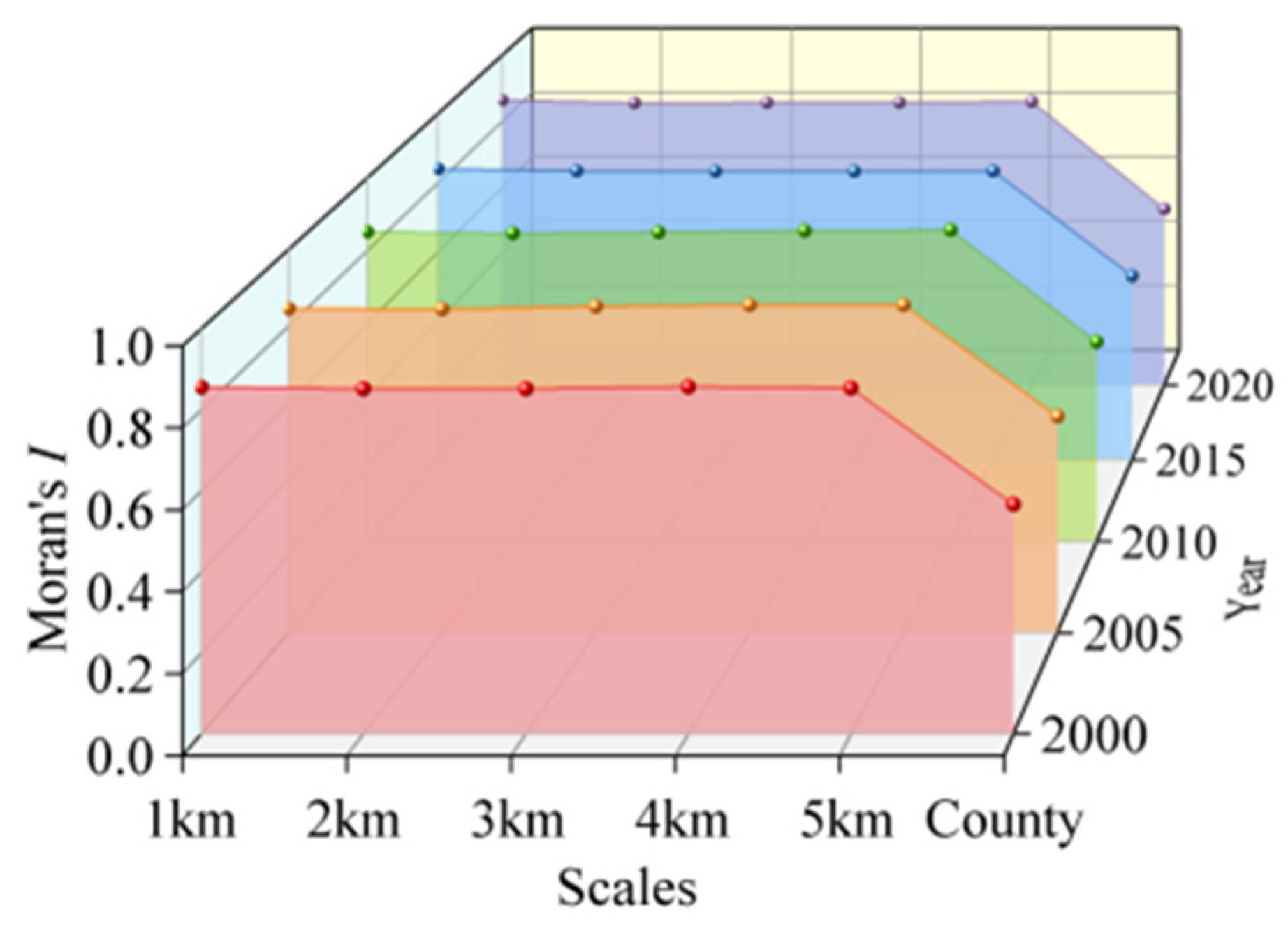
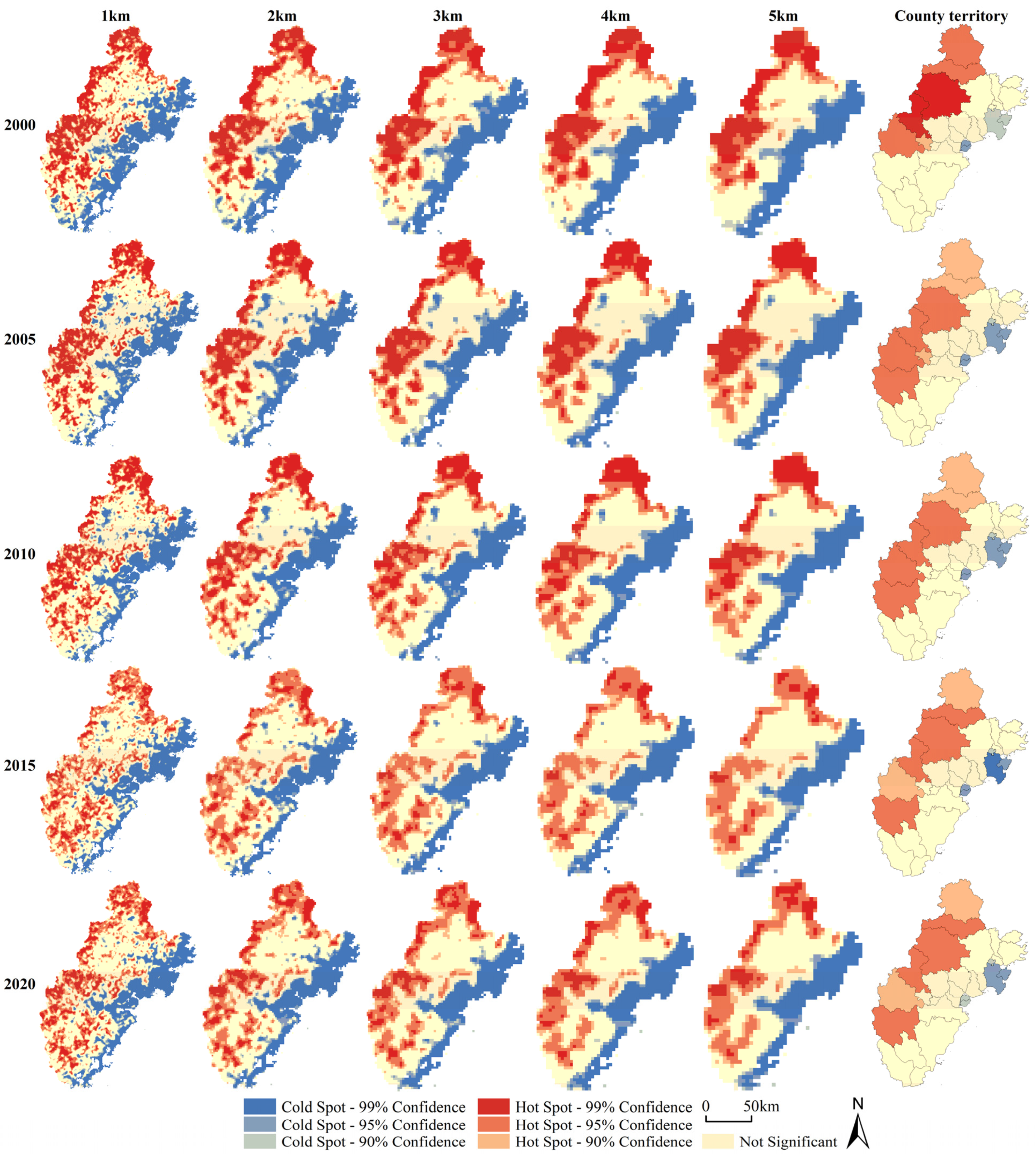
3.2. Spatial Cluster of EQ

Moran’s I was calculated as more than 0.53 at the county scale and more than 0.83 at different grid cell scales (Figure 6). This indicates that the RSEI has a significant positive spatial correlation. In addition, the RSEI has more significant aggregation characteristics on the fine study scales than on the coarser study scales, and it is significantly better than on the county scale.

From the results of the different grid scales, the cold and hot spots were spatially clustered (Figure 7). The hotspots were mainly distributed in the north and west, which indicated that high RSEI values were concentrated in this area and that the EQ was better. The cold spots were mainly located in the northeast, suggesting that low RSEI values were clustered in these areas with a poor EQ. In general, the numbers and spatial extent of hot and cold spots gradually decreased from 2000 to 2020.

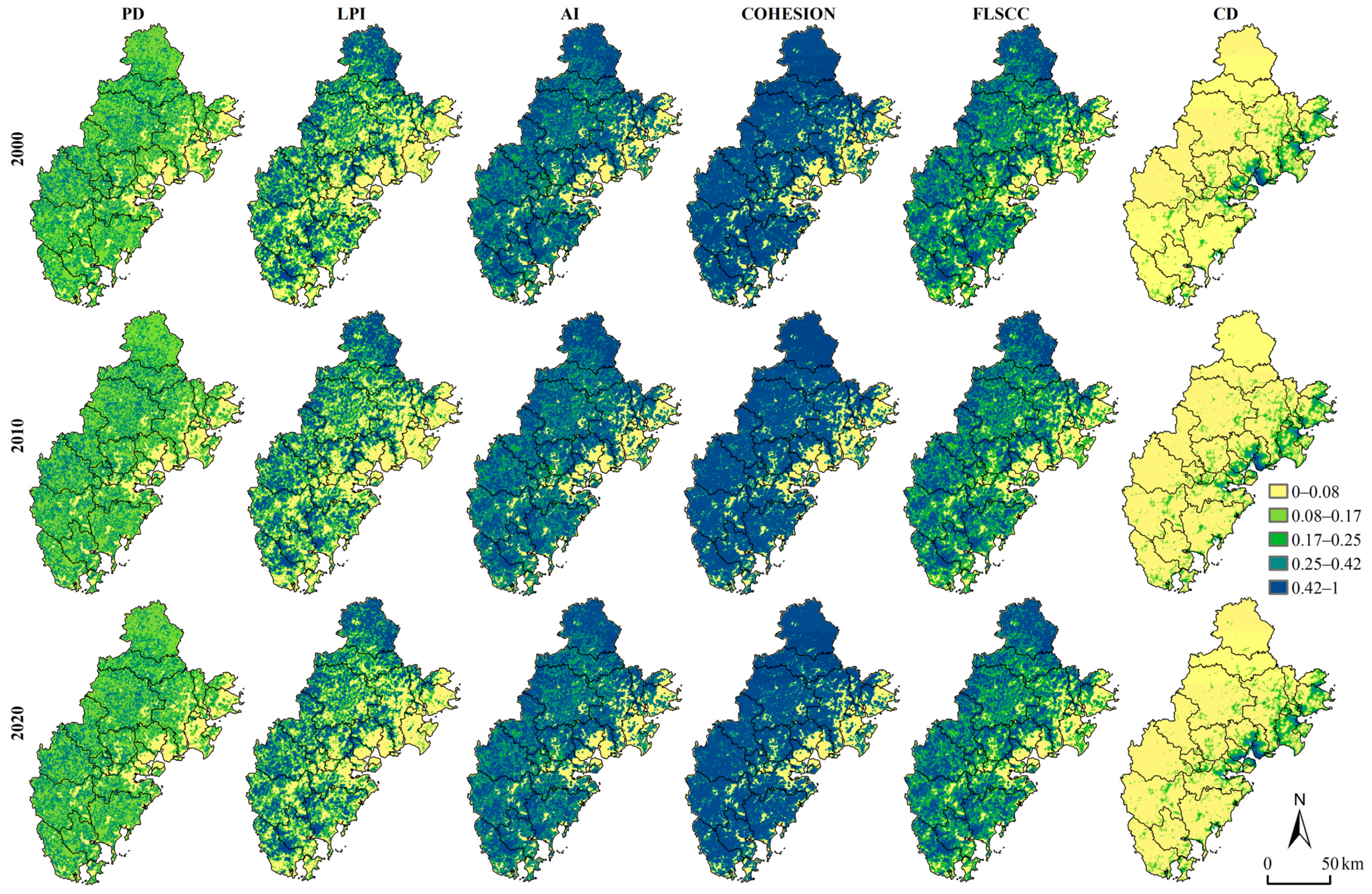
3.3. Spatiotemporal Changes in Forest Landscape Structural and Functional Connectivity

In general, the spatial distribution of PD, AI, LPI, COHESION, and FLSCC is similar, showing a decrease from the northwest to southeast (Figure 8). High values were mainly located in the west, south, and north, where the forest coverage rate was high with less human interference and higher structural connectivity of the landscape. In contrast, low values were predominantly found in the highly urbanized, human-intensive eastern part of the region, which has flat topography and low structural connectivity of the forest landscape. Low values of the CD were predominantly located in the north, west, and south, where the vegetation cover was higher, the distance from roads and construction land was greater, and the functional connectivity of the forest landscape was higher. High values of the CD were predominantly located in the east, where the road network was well-developed and the functional connectivity of the forest landscape was low.

Table 2. The changes in the forest landscape connectivity index from 2000 to 2020.

Year	Type of Change	PD	AI	LPI	COHESION	FLSCC	CD
	Increase	1.7%	0.2%	0.7%	0.2%	1.1%	1%
2000–2010	Stable	97.4%	99%	99.1%	98.9%	97.8%	98.9%
	Decrease	0.9%	0.8%	0.2%	0.9%	1.1%	0.1%
	Increase	0.6%	0.2%	0.2%	0.2%	0.3%	0.5%
2010–2020	Stable	99.1%	99.4%	99.1%	99.4%	99.1%	98.9%
	Decrease	0.3%	0.4%	0.7%	0.4%	0.6%	0.6%
	Increase	2.2%	0.3%	0%	0.4%	1.1%	0.9%
2000–2020	Stable	96.6%	98.6%	100%	98.4%	97.6%	98.9%
	Decrease	1.2%	1.1%	0%	1.3%	1.3%	0.2%

shows the temporal changes in the forest landscape structural connectivity index. Among them, from 2000 to 2020, the unchanged FLSCC area still accounts for the majority (97.6%) of the Fujian Delta region, while FLSCC increases in 1.1% of the region and decreases in 1.3%. The results for PD, AI, LPI, COHESION, and FLSCC are similar. The unchanged CD area still accounts for the majority (98.9%) of the Fujian Delta region, while the CD increased in 0.9% of the region and decreased in 0.2% of the region. These results indicate that the structural and functional connectivity of the forest landscape decreased by 1.3% and 0.9%, respectively, during 2000–2020.

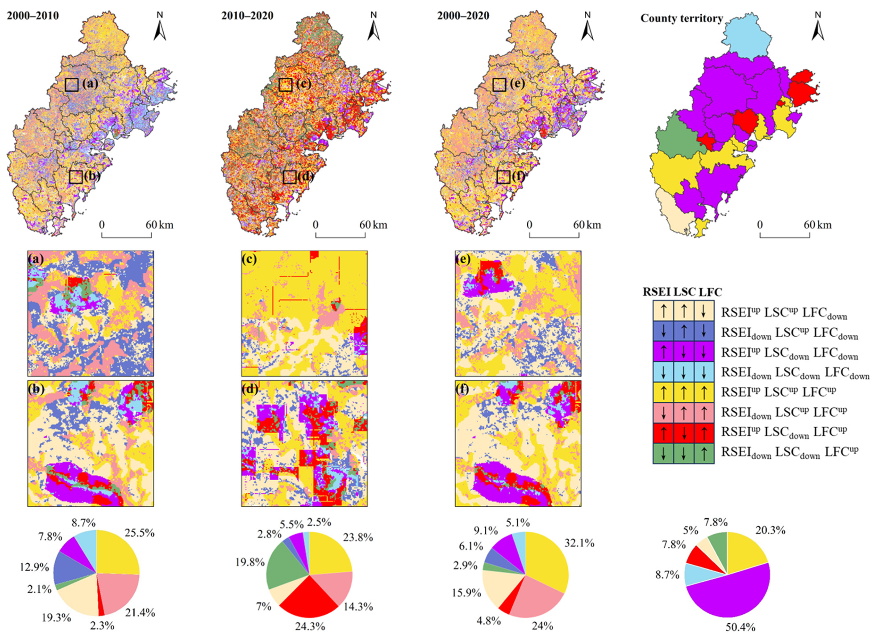
3.4. Changes in Pattern Recognition of EQ and Forest Landscape Structural and Function Connectivity

Based on the changes in RSEI and forest landscape connectivity (FLC) from 2000 to 2020, a two-dimensional framework was established to completely understand the changing dynamics of RSEI and FLC. The FLC was further subdivided into landscape structural connectivity (LSC) and functional connectivity (LFC). Based on the possible combinations of changes (increase or decrease) in the three components of RSEI, LSC, and LFC, this study identified eight patterns of changes in forest landscape structural and functional connectivity under the improvement or degradation of EQ and examined their area shares (Figure 9). The RSEI^upLSC^upLFC^up and RSEI_downLSC^upLFC^up modes occupied a large area (14.3%–32.1%) and were predominantly located in the south, north, and west. The RSEI^upLSC_downLFC^up mode (24.3%) was predominantly located in the east.

In addition, the framework was used to assess the dynamic pattern of RSEI and FLC at the county scale (Figure 9, Appendix S6). Taking the years between 2010 and 2020 as an example, most districts exhibited the following modes: RSEI^upLSC_downLFC_down mode (n = 13), RSEI^upLSC^upLFC^up mode (n = 7), and RSEI^upLSC_downLFC^up mode (n = 5). Only three counties showed a unique dynamic pattern of RSEI and FLC, as follows: RSEI_downLSC_downLFC_down (Dehua County), RSEI^upLSC^upLFC_down (Zhao’an County), and RSEI_downLSC_downLFC^up modes (Nanjing County).

3.5. Response of EQ to Forest Landscape Structural and Functional Connectivity

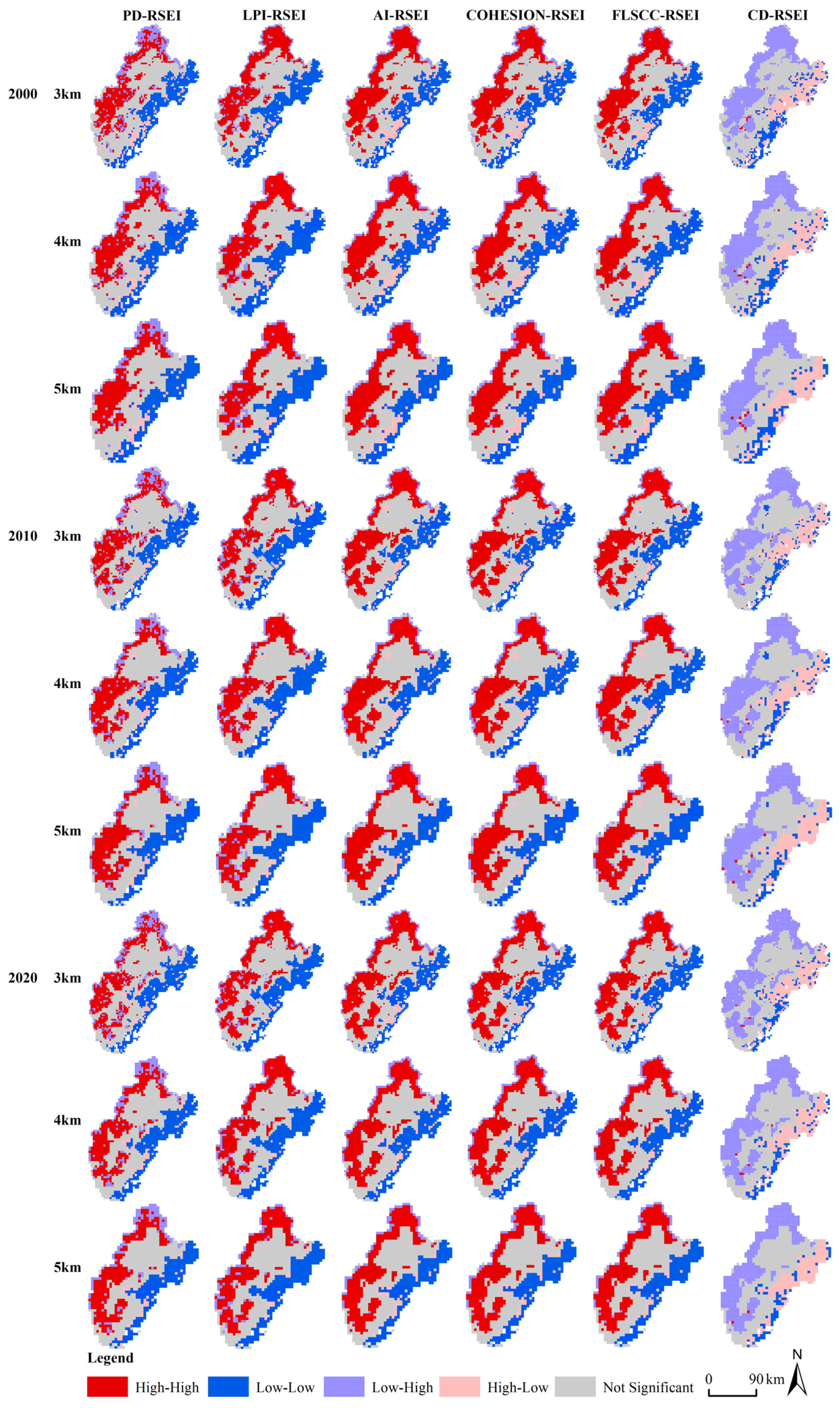
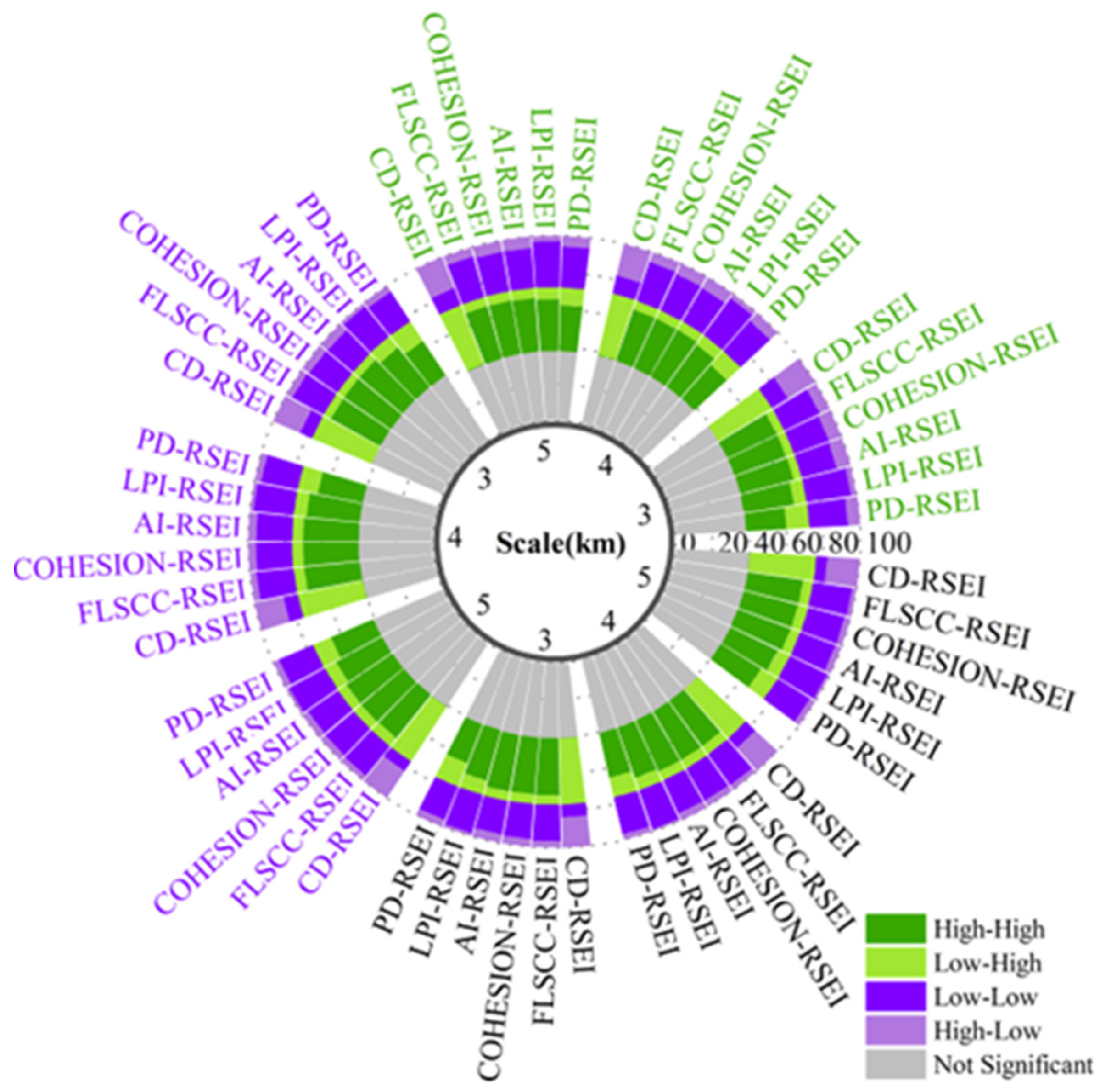
3.5.1. Bivariate Autocorrelation Analysis

Based on the above analysis of spatiotemporal changes in RSEI and FLC, the spatial correlation between the two was analyzed using bivariate spatial autocorrelation, with PD, LPI, AI, COHESION, FLSCC, and CD as the first variables and RSEI as the second variable. First, the forest landscape connectivity index and RSEI’s Moran’s I were calculated on five different scales (1, 2, 3, 4, and 5 km). Among them, the principle of choosing the scale of analysis was based on the following two reasons: first, Moran’s I index is the largest (

Table 3. Moran’s I of the forest landscape connectivity index and RSEI at different scales.

Year	Variable	Scales/km
		1	2	3	4	5
	PD–RSEI	0.30	0.37	0.42	0.45	0.48
	LPI–RSEI	0.59	0.58	0.59	0.60	0.62
2000	AI–RSEI	0.48	0.48	0.50	0.51	0.53
	COHESION–RSEI	0.49	0.49	0.51	0.52	0.53
	FLSCC–RSEI	0.54	0.53	0.55	0.55	0.57
	CD–RSEI	−0.42	−0.43	−0.44	−0.43	−0.44
	PD–RSEI	0.34	0.40	0.44	0.47	0.50
	LPI–RSEI	0.59	0.58	0.59	0.61	0.62
2010	AI–RSEI	0.53	0.53	0.54	0.55	0.56
	COHESION–RSEI	0.54	0.53	0.54	0.55	0.57
	FLSCC–RSEI	0.58	0.56	0.57	0.58	0.59
	CD–RSEI	−0.50	−0.51	−0.51	−0.50	−0.51
	PD–RSEI	0.39	0.45	0.49	0.52	0.54
	LPI–RSEI	0.60	0.59	0.61	0.62	0.64
2020	AI–RSEI	0.58	0.57	0.58	0.59	0.61
	COHESION–RSEI	0.58	0.57	0.59	0.60	0.61
	FLSCC–RSEI	0.62	0.60	0.62	0.62	0.64
	CD–RSEI	−0.56	−0.56	−0.56	−0.55	−0.56

), and second, additionally, R² is the largest and AIC is the smallest in the GWR analysis (Figure 10). Through comprehensive comparative research results and strict screening, the analytical scales of this study were selected as 3, 4, and 5 km.

From 2000 to 2020, the mean values of Moran’s I for these forest landscape structural connectivity indices and the RSEI were all greater than 0.42 at the 3, 4, and 5 km scales (Table 3), indicating that a significantly positive spatial correlation existed between them. The positive spatial correlation became more pronounced as the scale increased. The CD-RSEI Moran’s I was always less than −0.43, indicating that a significantly negative spatial correlation existed in CD-RSEI. With an increase in scale, the spatial negative correlation first decreased and then increased. Over time, the spatial aggregation effect was significantly enhanced.

In 2020, the FLSCC-RSEI aggregation type was dominated by high–high and low–low aggregations (Figure 11). The high–high aggregations were predominantly located in the north and west, with 31.0%, 30.3%, and 30.5% of the patches at the three scales (3, 4, and 5 km), respectively (Figure 12). The low–low aggregations were predominantly located in the northeastern and eastern regions, and the patches accounted for 19.9%, 20.5%, and 21.1% of the same three scales, respectively. This shows that with an increase in scale, the regions with high forest landscape structural connectivity and good EQ decreased and then increased, while the regions with low forest landscape structural connectivity and poor EQ increased. The structural connectivity index of the other forest landscapes was similar to that of the FLSCC. The CD-RSEI was dominated by low–high and high–low aggregations. The low–high aggregations were predominantly located in the north and west, and the proportion of patches under three scales (3, 4, and 5 km) was 35.8%, 35.6%, and 35.8%, respectively. The high–low aggregations were predominantly located in the northeastern and eastern regions, and the patches accounted for 16.5%, 16.6%, and 17.6% at the same three scales, respectively. This shows that with an increase in scale, the areas with a high functional connectivity of forest landscape and good EQ first decreased and then increased, while the areas with a low functional connectivity and poor EQ increased. In the other years, approximately similar changes were shown.

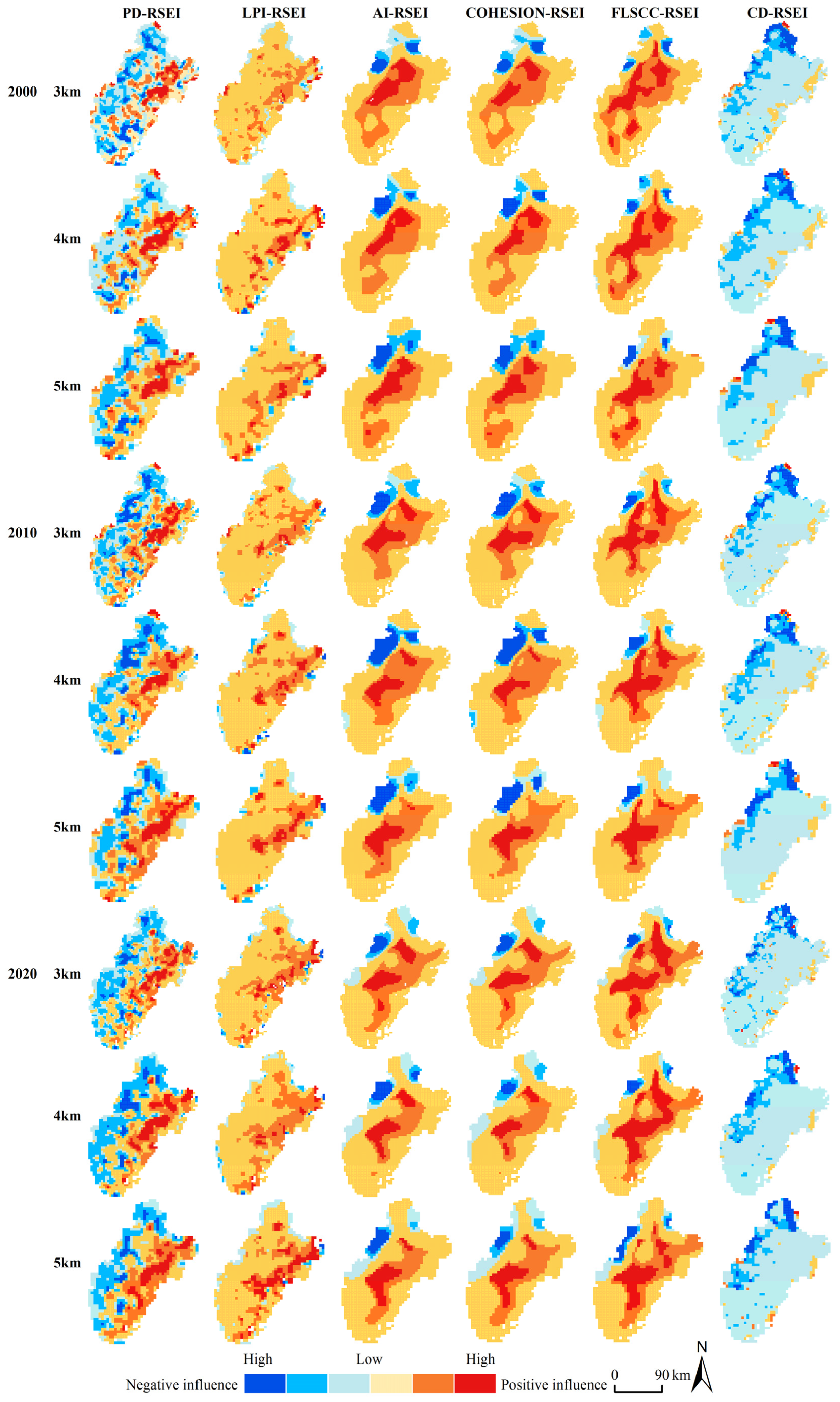
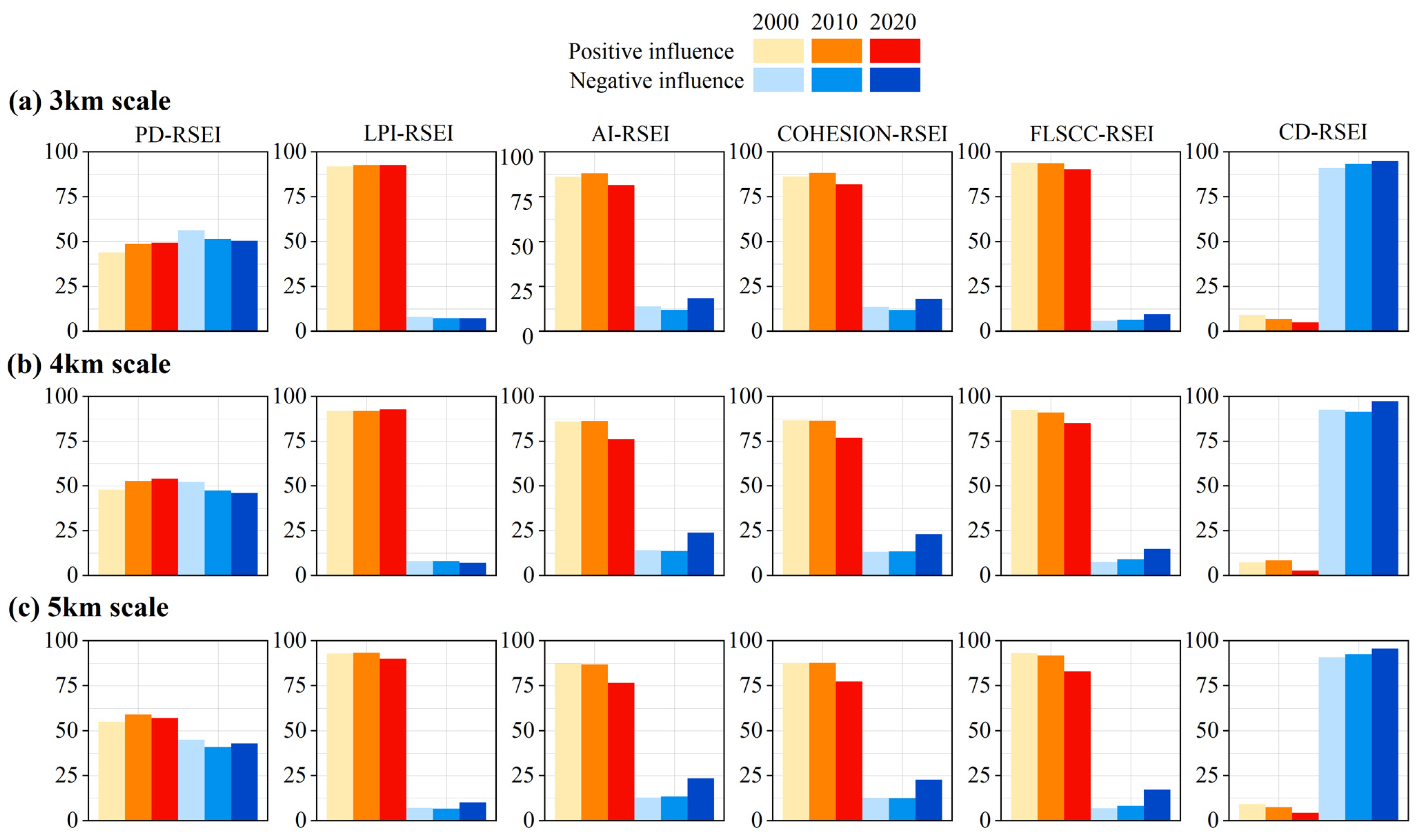
3.5.2. Geographically Weighted Regression Analysis

The GWR and OLS analyses were conducted for PD, LPI, AI, COHESION, FLSCC, CD, and RSEI from 2000 to 2020. To verify the applicability and accuracy of the GWR model, this model was compared with the OLS based on R² and AIC; the parameter estimations of the two models are shown in Figure 10. In 2020, from the perspective of model accuracy, the range in variation for R² in the OLS models of different scales was 0.27–0.58, and the interpretation and fitting accuracy of the GWR models of different scales was able to reach up to 97%. On all scales, the simulation effect of the GWR was greater than that of the OLS, and the AIC was smaller than that of the OLS. Therefore, the GWR model has more advantages than the traditional OLS model.

The GWR results showed spatial heterogeneity in forest landscape structural and functional connectivity effects on EQ at three spatial scales employed here (Figure 13). In 2020, at the 3 km scale specifically, the positive regression coefficient of PD-RSEI was predominantly located in the eastern region, and the negative regression coefficient was predominantly located in the northern and western regions. The effect of PD on RSEI was enhanced from the middle of the study area to the western and eastern regions. The positive regression coefficients of LPI-RSEI accounted for the majority, and a few regression coefficients were located in the marginal areas. The influence of LPI on RSEI gradually decreased from east to west. In addition, AI-RSEI, COHESION-RSEI, and FLSCC-RSEI had a similar distribution of regression coefficients, with positive regression coefficients mainly located in the southern and eastern regions and negative regression coefficients mainly located in the northern fringe regions. The influence of AI, COHESION, and FLSCC on RSEI gradually increased from south to north. The negative regression coefficients of CD-RSEI accounted for the majority, while a few regression coefficients were predominantly located in the east. The influence of CD on RSEI gradually decreased from north to south.

In terms of the area share of positive and negative regression coefficients at the 3, 4, and 5 km scales, LPI-RSEI, AI-RSEI, COHESION-RSEI, and FLSCC-RSEI were dominated by positive regression coefficients, and CD-RSEI was dominated by a negative regression coefficient (Figure 14). The PD-RSEI showed a negative effect at the 3 km scale, but the opposite effect at the 4 and 5 km scales. These results indicated that the spatial effects of these forest landscape structural connectivity indices on RSEI were mainly positive. The EQ was good when the forest landscape structural connectivity was high. In contrast, CD had a negative impact on RSEI. When the value of CD was low, the functional connectivity of the forest landscape was high, with a good EQ.

In 2020, from the mean absolute values of the forest landscape connectivity index and the RSEI regression coefficient (Appendix S7), at the scale of 3 km, the order of the strength of the influence relationship was as follows: CD-RSEI > FLSCC-RSEI > LPI-RSEI > AI-RSEI = COHESION-RSEI = PD-RSEI; at the scales of 4 and 5 km, it was as follows: CD-RSEI > PD-RSEI > FLSCC-RSEI = LPI-RSEI > AI-RSEI = COHESION-RSEI. The data for 2000 and 2010 were similar to the 2020 data. This shows that CD has the highest explanatory power to RSEI in different years and at different scales. The impact of forest landscape functional connectivity on EQ was greater than that of forest landscape structural connectivity.

4. Discussion

4.1. Spatiotemporal Evolution of EQ

According to the PCA of the four indicators calculated for 2000–2020 (Table 1), the indicators of greenness and wetness were positive, indicating that they contributed positively to EQ. The indicators of heat and dryness were negative, which suggests that they negatively influence EQ. These results are in line with earlier studies [59,76].

The present study found that the mean values of the RSEI between 2000 and 2020 ranged between 0.62 and 0.74 (corresponding to good levels of EQ, Figure 3), with a generally increasing trend in EQ. This was primarily the consequence of the Chinese government’s strategic decision in 2012 to vigorously promote the construction of an ecological civilization. However, the development demands of rapid urbanization and industrialization have encroached on pre-existing ecological land, resulting in an overall decline of 6.5% in the average RSEI value by 2020. This is consistent with the trend of previous studies on the EQ of urban agglomerations in China [77].

Next, the focus of environmental management at the county and district levels shifted to where the specific measures designed to improve the environment can be formulated in accordance with the actual ecological conditions of the districts and counties and in line with local conditions. For example, appropriately increasing the amount of forest vegetation and green belts around construction sites [78] helps to improve the regional EQ through a reasonable layout of landscape elements [29]. Therefore, this study calculated the average RSEI values for the twenty-eight county-level districts and counties (Figure 4).

The finding of spatial correlation in the distribution of RSEI as well as the spatial heterogeneity of RSEI at local scales is similar to the findings of earlier studies [62,77]. In addition, from the perspective of different scales, the spatial distribution of cold and hot spots of RSEI is similar, which is in agreement with the research results of Ji et al. [79].

4.2. Spatial Relationship between Forest Landscape Structural Connectivity Index and RSEI

The spatial distribution of forested landscapes was not continuous due to the marked differences in economic development in the study area. If the scale is too small, there will be many valueless pixels in the forest landscape index calculation; if the scale is too large, the spatial variation in the forest landscape index will be too smooth [80]. The optimal scale for this study was determined to be 3 km through a rigorous comparison of the bivariate spatial autocorrelation and GWR.

At the optimal scale (3 km), the mean regression coefficients of FLSCC-RSEI were larger than those of the individual structural connectivity index and RSEI (Table S4). This shows that FLSCC provides more explanatory power and advantages than a single landscape structural connectivity index because FLSCC integrates most of the information of the patch, aggregation, and connectivity indices, rendering it more objective and comprehensive in explaining its impact on RSEI. At the scales of 4 and 5 km, the explanatory power of PD to RSEI was stronger than that of FLSCC and LPI. This indicates that the patch index is sensitive to scale, and the results at different scales vary. The mean values of the regression coefficients of AI-RSEI and COHESION-RSEI are equal in different scales. This indicates that the aggregation and connectivity indices have the same explanatory power for RSEI, and both are insensitive to a change in scale [46].

Based on the above effects of a single landscape index and a comprehensive index on RSEI, this study provides a reference for selecting landscape indices in different regions for pattern change analysis, as follows: (1) if the influence of landscape connectivity on RSEI at an optimal scale is studied, FLSCC can be selected first; (2) if the influence of a single landscape index on RSEI at different scales is studied, PD and LPI can be preferentially selected; (3) if the impact of the landscape index on RSEI on a single scale is studied, AI and COHESION can be selected first. This discussion also shows that different landscape indices vary in both their applicability and sensitivity to scale change. This finding is similar to that of Li et al. [81]. This requires researchers in the actual operation process to choose an appropriate analysis method based on the research goal.

4.3. Effects of Forest Landscape Structural and Functional Connectivity on EQ

The four dynamic changes generated by a two-dimensional framework reflect the coupling change state of differences in RSEI and FLC. In the early stages of EQ degradation, irregular or small, the distant forest patches are cleared first, resulting in an RSEI_downFLC^up mode. As the forest loss spreads to large intact patches, more forest edges are created [6], which allows the display of an RSEI_downFLC_down mode. At this stage, the EQ has entered a state of deep degradation. In contrast, in the EQ improvement (ecological protection) scenario, the introduction of additional small forest patches results in an RSEI^upFLC_down mode with more forest patches, representing the initial stages of an improvement in EQ. This is mainly due to the widespread phenomenon of “spatial displacement of forests” in the context of China’s long-standing and prominent human–land conflict and the forest occupation and compensation balance system [5]. Until the small patches are connected to complete, large forest patches, showing the RSEI^upFLC^up mode with fewer forest patches, will represent the depth of the EQ improvement stage.

The eight change modes in the RSEI and forest landscape structural and functional connectivity were divided into the following two types: the structural and functional connectivity consistent type and the functional connectivity sensitive type. RSEI^upLSC^upLFC^up, RSEI^upLSC_downLFC_down, RSEI_downLSC^upLFC^up, and RSEI_downLSC_downLFC_down modes form the structural and functional connectivity consistent type. This indicates that when the EQ improves or deteriorates, the changes in the forest landscape’s structural and functional connectivity are consistent. RSEI^upLSC_downLFC^up, RSEI^upLSC^upLFC_down, and RSEI_downLSC_downLFC^up form the functional connectivity sensitive type. This indicates that while landscape structural connectivity will change correspondingly when EQ is either improved or degraded, the landscape functional connectivity is more sensitive to these changes and displays a broader range of changes (Appendix S8). Moreover, this finding also shows that the direction and amplitude of structural and functional connectivity changes are not synchronized, which is in agreement with the research results of Brennan et al. [42]. The two modes of RSEI_downLSC^upLFC^up and RSEI_downLSC^upLFC_down were not identified at the county scale, which may be attributed to the excessive scale of statistics at this scale, and makes the spatial changes appear to be too smooth. In addition, this research speculates that RSEI_downLSC^upLFC_down is also a functional connectivity-sensitive type. Even if the forest area remains the same, rapid urbanization will cause dramatic changes in land use, which may convert grassland or cultivated land into construction land. Then, the corresponding resistance factor increases and the functional connectivity decreases, even if the structural connectivity is unchanged. However, the Chinese government vigorously promotes the development of an ecologically sound civilization, and it has implemented a string of environmental restoration works and the policy of returning farmland to forest and grassland [62]. For example, when cultivated land or unused land becomes grassland, the resistance factor decreases and the structural connectivity remains unchanged; as a result, the functional connectivity will increase.

The change modes were classified so that 79.4% of the area belongs to the consistent type of structural and functional connectivity and 20.6% of the area belongs to the functional connectivity sensitive type (Figure 9). No structural connection-sensitive type has been found on the scale of districts and counties. Therefore, in general, compared with the landscape structural connectivity represented by the landscape index, the landscape functional connectivity represented by CD has more advantages, which is consistent with the research results of Liu et al. [64].

The similarity between the structural and functional connectivity shows that both can be used to measure the structure of the landscape. The difference is that functional connectivity accounts for the ecological process on the basis of structural connectivity [40], which makes it more scientifically sound and reasonable. However, this does not imply that landscape functional connectivity can completely replace landscape structural connectivity. Because studying ecological processes and functions requires considerable energy and time, scholars can often reflect different landscape ecological processes and functions through the study of the spatial distribution of landscape elements. Therefore, the study of landscape connectivity is still inseparable from the analysis of landscape structural units. The researcher must choose the appropriate landscape connectivity measurement method based on the specific situation in the actual application process.

Based on the above RSEI and the analysis of the change pattern of forest landscape structural and functional connectivity, this study provides references for selecting appropriate landscape connectivity measurement methods at different regional scales for analysis, that is, (1) if the forest landscape connectivity in areas with relatively flat terrain and high urbanization is studied, CD can be preferred [64]; (2) if the forest landscape connectivity in areas with higher elevations and less human disturbance is studied, both the landscape index and CD can be selected.

This study mainly analyzed the impact of the two important factors of forest landscape structural and functional connectivity on EQ. In the bivariate spatial autocorrelation (Figure 11), the similarity between these two lies in the positive correlation between PD, AI, LPI, COHESION, FLSCC, and RSEI and the negative correlation between CD and RSEI, which are consistent in spatial superposition. Consistent places were often distributed in the northern and western regions. The forest landscape structure and function in these areas are highly connected, the elevation is higher with less human interference, and the environment is rich with a better EQ. Another part is located along the eastern and northeastern coasts. In this region, the forest landscape structure and function are poorly connected with high levels of urbanization [82] and population density with a well-developed road network, so the environment is under a certain amount of pressure with a poor EQ. These results are in accordance with the findings of previously performed studies [83]. The difference between the two is, first, the percentage of patches in the main aggregation types. The PD, AI, LPI, COHESION, FLSCC, and RSEI were dominated by high–high and low–low aggregations, while the CD-RSEI was dominated by low–high and high–low aggregations. Second, the spatial distribution of the main aggregations is different. The high–high aggregations of PD, AI, LPI, COHESION, FLSCC, and RSEI were located in the west and north, and the low–low aggregations were distributed in the east and northeast. The low–high aggregations of CD-RSEI were located in the west and north, and the high–low aggregations were distributed in the east and northeast. With the increase in scale, the patch proportions of PD, AI, LPI, COHESION, FLSCC, CD, and RSEI both increased and decreased (Figure 12). This also confirmed the existence of the landscape metric scale effect [80], indicating that the size of the analysis scale will affect the research findings.

In GWR, the positive regression coefficients of RSEI and the forest landscape structural and functional connectivity index were not completely consistent in spatial superposition (Figure 13). The consistent area was located in the northeast where the built-up area is dense and the forest cover is low. There were inconsistencies identified in the east, where the structural and functional connectivity of the forest landscape was low and the EQ was poor. The negative regression coefficients were not completely consistent in the spatial superposition. The spatial superposition of a consistent negative regression coefficient is located in the northern region. However, inconsistencies were found in the southern region, where the structural and functional connectivity of the forest landscape was high with a good EQ.

In areas with a poor EQ, such as construction land in the east, the PD-RSEI regression coefficient was positive (Figure 13). In contrast, the regression coefficient was negative in the regions where the EQ was mainly either excellent or good, such as the forest and grassland in the west and northwest. This finding is similar to that of Yang et al. [29]. The fragmentation of forest patches in areas with high forest cover led to reduced landscape connectivity, which negatively affected the EQ. The fragmentation of forest patches with low forest cover has led to an increase in green spaces within construction land, including roadside greenbelts. These green spaces significantly contribute to improving the city’s EQ.

4.4. Limitations and Implications

This study suggests that increasing landscape connectivity is beneficial to improving the EQ [29]. The impact of changing landscape connectivity on the regional EQ cannot be ignored. The direction and degree of its influence varied greatly from region to region, and the degree of influence varied with scale, which was also illustrated by the distinct scale effect of landscape connectivity on the influence of EQ. As noted in previous studies, it is imperative to include a functional connectivity component in habitat fragmentation studies [84]. Therefore, this study emphasized that the rational allocation of landscape elements in enhancing landscape connectivity should be considered when developing landscape management strategies. In particular, this should primarily increase the functional connectivity of the landscape. In addition, it is vital to focus on the spatial relationship between landscape configurations and the environment and it is also necessary to curb deforestation, so as to increase the resistance of the ecosystem and to realize the protection of biodiversity and the development of an ecologically sound civilization.

The innovation of this study lies in that, first, the landscape connectivity is measured from the perspective of structure and function, and the analysis is more comprehensive, which compensates for the shortcomings of only considering structural connectivity or functional connectivity in the past. Second, at different scales, the response of EQ to forest landscape structural and functional connectivity is fully revealed. Through the study of the relationship between EQ at different scales and the forest landscape structural and functional connectivity, we can explore the change patterns of EQ and forest landscape structural and functional connectivity at different spatial scales, allowing the identification of trends and patterns that may not be obvious on a single scale. Some changes may only become apparent on larger scales, while others may only appear on smaller scales. This multi-spatiotemporal scale approach helps to identify complex spatial relationships. In addition, the inclusion of multiple temporal and spatial scales reduces the risk of drawing erroneous conclusions based on the uniqueness of a single scale, thereby enhancing the scientific and robust nature of the findings. Finally, eight forest landscape structural and functional connectivity change modes were detected under the conditions of improving or degrading the EQ based on the change in RSEI and forest landscape structural and functional connectivity. This study provides a scientific reference for ecological environment monitoring and the conservation decision-making of managers.

However, this study has some limitations. First, only four common resistance factors were considered in the construction of the CD. Animal movements and landscape connectivity needs have been shown to potentially be either directly or indirectly affected by climate change [42]. Future research could explore the effects of temperature and precipitation on landscape connectivity. Second, EQ is affected by a combination of factors [83]. This study is concerned with the effect of forest landscape connectivity on EQ. Meanwhile, the socio-economic, topographical, and meteorological factors of the region have not been studied. Other factors influencing the results should be taken into account in subsequent studies with a view to obtaining more comprehensive and objective analytical results. Finally, a two-dimensional framework was established based on EQ and forest landscape connectivity changes, and eight change patterns were identified, which were applied only at the county scale. Future studies could perform more detailed analyses at different grid scales and compare the results at those scales.

5. Conclusions

This study analyzed the spatiotemporal changes in EQ and explored the response of EQ to forest landscape structural and functional connectivity. From the landscape structural and functional connectivity perspective, reasonable suggestions for protecting and improving EQ were put forward. The purpose of this study is to provide valuable insights into ecological environment monitoring and the ecological conservation decision-making of managers. The main conclusions of this study are as follows:

(1)

From 2000 to 2020, the overall EQ increased, improving in 37.5% of the region and deteriorating in 13.8% of the region. RSEI has a significant spatial positive correlation at different scales. The hot spots of the RSEI were predominantly located in the western and northern regions, and the cold spots were predominantly in the northeastern region.

(2)

The forest landscape structural and functional connectivity shows a small decreasing trend from 2000 to 2020, decreasing by 1.3% and 0.9%, respectively.

(3)

Eight forest landscape structural and functional connectivity change modes were detected under the conditions of an improving or degrading EQ based on the change in RSEI, forest landscape structural, and functional connectivity.

(4)

From the bivariate spatial autocorrelation, FLSCC-RSEI was dominated by high–high and low–low aggregation and CD-RSEI was dominated by low–high and high–low aggregation. The GWR results showed that CD had the highest explanatory power to RSEI in different scales. The impact of the forest landscape functional connectivity on EQ is greater than that of the forest landscape structural connectivity, and the impact magnitude is different. The negative regression coefficients of CD-RSEI accounted for the majority; meanwhile, a few regression coefficients were predominantly located in the east.

References

1. Fischer, R.; Taubert, F.; Müller, M.S.; Groeneveld, J.; Lehmann, S.; Wiegand, T.; Huth, A. Accelerated forest fragmentation leads to critical increase in tropical forest edge area. Sci. Adv. 2021, 7, eabg7012. [Google Scholar] [CrossRef]
2. Modica, G.; Praticò, S.; Laudari, L.; Ledda, A.; Di Fazio, S.; De Montis, A. Implementation of multispecies ecological networks at the regional scale: Analysis and multi–temporal assessment. J. Environ. Manag. 2021, 289, 112494. [Google Scholar] [CrossRef]
3. Zou, L.L.; Wang, J.Y.; Bai, M.D. Assessing spatial–temporal heterogeneity of China’s landscape fragmentation in 1980–2020. Ecol. Indicat. 2022, 136, 108654. [Google Scholar] [CrossRef]
4. Matricardi, E.A.T.; Skole, D.L.; Costa, O.B.; Pedlowski, M.A.; Samek, J.H.; Miguel, E.P. Long–term forest degradation surpasses deforestation in the Brazilian Amazon. Science 2020, 369, 1378–1382. [Google Scholar] [CrossRef]
5. Zhen, S.Y.; Zhao, Q.; Liu, S.; Wu, Z.L.; Lin, S.; Li, J.; Hu, X.S. Detecting Spatiotemporal Dynamics and Driving Patterns in Forest Fragmentation with a Forest Fragmentation Comprehensive Index (FFCI): Taking an Area with Active Forest Cover Change as a Case Study. Forests 2023, 14, 1135. [Google Scholar] [CrossRef]
6. Ma, J.; Li, J.W.; Wu, W.B.; Liu, J.J. Global forest fragmentation change from 2000 to 2020. Nat. Commun. 2023, 14, 3752. [Google Scholar] [CrossRef] [PubMed]
7. Kindu, M.; Schneider, T.; Teketay, D.; Knoke, T. Changes of ecosystem service values in response to land use/land cover dynamics in Munessa–Shashemene landscape of the Ethiopian highlands. Sci. Total Environ. 2016, 547, 137–147. [Google Scholar] [CrossRef]
8. Ren, Y.; Deng, L.Y.; Zuo, S.D.; Lou, Y.J.; Shao, G.F.; Wei, X.H.; Hua, L.Z.; Yang, Y.S. Geographical modeling of spatial interaction between human activity and forest connectivity in an urban landscape of southeast China. Landsc. Ecol. 2014, 29, 1741–1758. [Google Scholar] [CrossRef]
9. Che, L.; Yin, S.; Jin, J.; Wu, W. Assessment and Simulation of Urban Ecological Environment Quality Based on Geographic Information System Ecological Index. Land 2024, 13, 687. [Google Scholar] [CrossRef]
10. Liu, H.; Weng, Q.H. Seasonal variations in the relationship between landscape pattern and land surface temperature in Indianapolis, USA. Environ. Monitor. Assess. 2008, 144, 199–219. [Google Scholar] [CrossRef]
11. Liu, C.J.; Zhang, F.; Johnson, V.C.; Duan, P.; Kung, H.T. Spatio–temporal variation of oasis landscape pattern in arid area: Human or natural driving? Ecol. Indicat. 2021, 125, 107495. [Google Scholar] [CrossRef]
12. Peng, Y.; Wang, Q.H.; Bai, L. Identification of the key landscape metrics indicating regional temperature at different spatial scales and vegetation transpiration. Ecol. Indicat. 2020, 111, 106066. [Google Scholar] [CrossRef]
13. Crompton, O.; Corrêa, D.; Duncan, J.; Thompson, S. Deforestation–induced surface warming is influenced by the fragmentation and spatial extent of forest loss in Maritime Southeast Asia. Environ. Res. Lett. 2021, 16, 114018. [Google Scholar] [CrossRef]
14. Li, Y.; Kang, W.; Han, Y.; Song, Y. Spatial and temporal patterns of microclimates at an urban forest edge and their management implications. Environ. Monitor. Assess. 2018, 190, 93. [Google Scholar] [CrossRef] [PubMed]
15. Hu, X.S.; Xu, H.Q. A new remote sensing index for assessing the spatial heterogeneity in urban ecological quality: A case from Fuzhou City, China. Ecol. Indicat. 2018, 89, 11–21. [Google Scholar] [CrossRef]
16. Gupta, K.; Kumar, P.; Pathan, S.K.; Sharma, K.P. Urban Neighborhood Green Index—A measure of green spaces in urban areas. Urban Plann. 2012, 105, 325–335. [Google Scholar] [CrossRef]
17. Ivits, E.; Cherlet, M.; Mehl, W.; Sommer, S. Estimating the ecological status and change of riparian zones in Andalusia assessed by multi–temporal AVHHR datasets. Ecol. Indicat. 2009, 9, 422–431. [Google Scholar] [CrossRef]
18. Imhoff, M.L.; Zhang, P.; Wolfe, R.E.; Bounoua, L. Remote sensing of the urban heat island effect across biomes in the continental USA. Remote Sens. Environ. 2010, 114, 504–513. [Google Scholar] [CrossRef]
19. Zarch, M.A.A.; Malekinezhad, H.; Mobin, M.H.; Dastorani, M.T.; Kousari, M.R. Drought Monitoring by Reconnaissance Drought Index (RDI) in Iran. Water Resour. Manag. 2011, 25, 3485–3504. [Google Scholar] [CrossRef]
20. Xiong, Y.; Xu, W.H.; Lu, N.; Huang, S.D.; Wu, C.; Wang, L.G.; Dai, F.; Kou, W.L. Assessment of spatial–temporal changes of ecological environment quality based on RSEI and GEE: A case study in Erhai Lake Basin, Yunnan province, China. Ecol. Indicat. 2021, 125, 107518. [Google Scholar] [CrossRef]
21. Zhao, Y.W.; Zhou, L.Q.; Dong, B.Q.; Dai, C. Health assessment for urban rivers based on the pressure, state and response framework—A case study of the Shiwuli River. Ecol. Indicat. 2019, 99, 324–331. [Google Scholar] [CrossRef]
22. Yu, H.D.; Zhao, J.J. The Impact of Environmental Conditions on Urban Eco–Sustainable Total Factor Productivity: A Case Study of 21 Cities in Guangdong Province, China. Int. J. Environ. Res. Public Health 2020, 17, 1329. [Google Scholar] [CrossRef] [PubMed]
23. Lv, Y.; Xiu, L.A.; Yao, X.J.; Yu, Z.P.; Huang, X.Y. Spatiotemporal evolution and driving factors analysis of the eco–quality in the Lanxi urban agglomeration. Ecol. Indicat. 2023, 156, 111114. [Google Scholar] [CrossRef]
24. Xu, H. A remote sensing urban ecological index and its application. Acta Ecol. Sin. 2013, 33, 7853–7862. [Google Scholar]
25. An, M.; Xie, P.; He, W.J.; Wang, B.; Huang, J.; Khanal, R. Local and tele–coupling development between carbon emission and ecologic environment quality. J. Clean. Prod. 2023, 394, 136409. [Google Scholar] [CrossRef]
26. Firozjaei, M.K.; Kiavarz, M.; Homaee, M.; Arsanjani, J.J.; Alavipanah, S.K. A novel method to quantify urban surface ecological poorness zone: A case study of several European cities. Sci. Total Environ. 2021, 757, 143755. [Google Scholar] [CrossRef] [PubMed]
27. Sun, J.; Hu, Y.; Li, Y.; Weng, L.F.; Bai, H.A.; Meng, F.D.; Wang, T.; Du, H.Z.; Xu, D.; Lu, S. A temporospatial assessment of environmental quality in urbanizing Ethiopia. J. Environ. Manag. 2023, 332, 117431. [Google Scholar] [CrossRef] [PubMed]
28. Zhang, K.L.; Feng, R.R.; Zhang, Z.C.; Deng, C.; Zhang, H.J.; Liu, K. Exploring the Driving Factors of Remote Sensing Ecological Index Changes from the Perspective of Geospatial Differentiation: A Case Study of the Weihe River Basin, China. Int. J. Environ. Res. Public Health 2022, 19, 10930. [Google Scholar] [CrossRef] [PubMed]
29. Yang, H.H.; Xu, W.Z.; Yu, J.; Xie, X.Q.; Xie, Z.Q.; Lei, X.Y.; Wu, Z.K.; Ding, Z. Exploring the impact of changing landscape patterns on ecological quality in different cities: A comparative study among three megacities in eastern and western China. Ecol. Inform. 2023, 77, 102255. [Google Scholar] [CrossRef]
30. Lin, L.L.; Hao, Z.B.; Post, C.J.; Mikhailova, E.A. Monitoring Ecological Changes on a Rapidly Urbanizing Island Using a Remote Sensing–Based Ecological Index Produced Time Series. Remote Sens. 2022, 14, 5773. [Google Scholar] [CrossRef]
31. Yang, L.Q.; Yu, K.Y.; Ai, J.W.; Liu, Y.F.; Lin, L.L.; Lin, L.C.; Liu, J. The Influence of Green Space Patterns on Land Surface Temperature in Different Seasons: A Case Study of Fuzhou City, China. Remote Sens. 2021, 13, 5114. [Google Scholar] [CrossRef]
32. Bird, K.I.T.; Uden, D.R.; Allen, C.R. Functional connectivity varies across scales in a fragmented landscape. PLoS ONE 2023, 18, e0289706. [Google Scholar] [CrossRef]
33. Taylor, P.; Fahrig, L.; Henein, K.; Merriam, G. Connectivity is a vital element of landscape structure. Oikos 1993, 68, 571–573. [Google Scholar] [CrossRef]
34. Morin, E.; Razafimbelo, N.T.; Yengué, J.L.; Guinard, Y.; Grandjean, F.; Bech, N. Are human–induced changes good or bad to dynamic landscape connectivity? J. Environ. Manag. 2024, 352, 120009. [Google Scholar] [CrossRef]
35. Li, W.W.; Liu, P.; Yang, N.; Chen, S.; Guo, X.M.; Wang, B.; Zhang, L. Improving landscape connectivity through habitat restoration: Application for Asian elephant conservation in Xishuangbanna Prefecture, China. Integr. Zool. 2023, 19, 319–335. [Google Scholar] [CrossRef]
36. Zhang, C.; Chen, W.B.; He, L.; Huang, F.F.; Li, H.F. Dynamic simulation of the grassland connectivity and the effects of landscape pattern in China’s Poyang Lake from the integrated perspective of habitat and biology. Ecohydrology 2023, 16, e2540. [Google Scholar] [CrossRef]
37. Lee, J.; Ellis, C.D.; Choi, Y.E.; You, S.; Chon, J. An Integrated Approach to Mitigation Wetland Site Selection: A Case Study in Gwacheon, Korea. Sustainability 2015, 7, 3386–3413. [Google Scholar] [CrossRef]
38. Adriaensen, F.; Chardon, J.P.; De Blust, G.; Swinnen, E.; Villalba, S.; Gulinck, H.; Matthysen, E. The application of ‘least–cost’ modelling as a functional landscape model. Urban Plann. 2003, 64, 233–247. [Google Scholar] [CrossRef]
39. Gómez, A.Q.; Rivas, C.A.; González–Moreno, P.; Navarro–Cerrillo, R.M. Forest plantations in Manabi (Ecuador): Assessment of fragmentation and connectivity to support dry tropical forests conservation. Appl. Sci. 2023, 13, 6418. [Google Scholar] [CrossRef]
40. Zhang, C.; Chen, W.B.; Huang, F.F.; He, L.; Li, H.F. Dynamic simulation of functional connectivity and identification of conservation priorities for grassland in China’s Poyang Lake considering ecological processes. Ecol. Indicat. 2023, 149, 110163. [Google Scholar] [CrossRef]
41. Belote, R.T.; Barnett, K.; Zeller, K.; Brennan, A.; Gage, J. Correction to: Examining local and regional ecological connectivity throughout North America. Landsc. Ecol. 2023, 38, 1619–1620. [Google Scholar] [CrossRef]
42. Brennan, A.; Naidoo, R.; Greenstreet, L.; Mehrabi, Z.; Ramankutty, N.; Kremen, C. Functional connectivity of the world’s protected areas. Science 2022, 376, 1101–1104. [Google Scholar] [CrossRef]
43. Almasieh, K.; Mohammadi, A. Assessing landscape suitability and connectivity for effective conservation of two semi–desert ungulates in Iran. Cons. Sci. Pract. 2023, 12, e13047. [Google Scholar] [CrossRef]
44. Gonzalez, J.R.; del Barrio, G.; Duguy, B. Assessing functional landscape connectivity for disturbance propagation on regional scales—A cost–surface model approach applied to surface fire spread. Ecol. Model. 2008, 211, 121–141. [Google Scholar] [CrossRef]
45. Zhou, W.; Cao, F.L. Effects of changing spatial extent on the relationship between urban forest patterns and land surface temperature. Ecol. Indicat. 2020, 109, 105778. [Google Scholar] [CrossRef]
46. Li, X.M.; Zhou, W.Q.; Ouyang, Z.Y. Relationship between land surface temperature and spatial pattern of greenspace: What are the effects of spatial resolution? Urban Plann. 2013, 114, 1–8. [Google Scholar] [CrossRef]
47. Wang, L.Y.; Hou, H.; Weng, J.X. Ordinary least squares modelling of urban heat island intensity based on landscape composition and configuration: A comparative study among three megacities along the Yangtze River. Sustain. Cities Soc. 2020, 62, 102381. [Google Scholar] [CrossRef]
48. Su, S.L.; Xiao, R.; Zhang, Y. Multi–scale analysis of spatially varying relationships between agricultural landscape patterns and urbanization using geographically weighted regression. Appl. Geogr. 2012, 32, 360–375. [Google Scholar] [CrossRef]
49. Wang, H.; Zang, F.; Zhao, C.Y.; Liu, C.L. A GWR downscaling method to reconstruct high–resolution precipitation dataset based on GSMaP–Gauge data: A case study in the Qilian Mountains, Northwest China. Sci. Total Environ. 2022, 810, 152066. [Google Scholar] [CrossRef]
50. Tian, A.H.; Xu, T.T.; Gao, J.Y.; Liu, C.; Han, L.T. Multi–scale spatiotemporal wetland loss and its critical influencing factors in China determined using innovative grid–based GWR. Ecol. Indicat. 2023, 149, 110144. [Google Scholar] [CrossRef]
51. Wu, D.C. Spatially and temporally varying relationships between ecological footprint and influencing factors in China’s provinces Using Geographically Weighted Regression (GWR). J. Clean. Prod. 2020, 261, 121089. [Google Scholar] [CrossRef]
52. Zheng, X.C.; Zou, Z.Y.; Xu, C.M.; Lin, S.; Wu, Z.L.; Qiu, R.Z.; Hu, X.S.; Li, J. A New Remote Sensing Index for Assessing Spatial Heterogeneity in Urban Ecoenvironmental–Quality–Associated Road Networks. Land 2022, 11, 46. [Google Scholar] [CrossRef]
53. Li, S.A.; An, W.Z.; Zhang, J.; Gan, M.Y.; Wang, K.; Ding, L.L.; Li, W.Q. Optimizing limit lines in urban–rural transitional areas: Unveiling the spatial dynamics of trade–offs and synergies among land use functions. Habitat Int. 2023, 140, 102907. [Google Scholar] [CrossRef]
54. Lin, J.H.; Lin, M.S.; Chen, W.H.; Zhang, A.; Qi, X.H.; Hou, H.R. Ecological risks of geological disasters and the patterns of the urban agglomeration in the Fujian Delta region. Ecol. Indicat. 2021, 125, 107475. [Google Scholar] [CrossRef]
55. Liu, X.; Zeng, S.P.; Namaiti, A.; Xin, R.H. Comparison between three convolutional neural networks for local climate zone classification using Google Earth Images: A case study of the Fujian Delta in China. Ecol. Indicat. 2023, 148, 110086. [Google Scholar] [CrossRef]
56. Chen, Y.P.; Peng, L.H.; Cao, W.Z. Health evaluation and coordinated development characteristics of urban agglomeration: Case study of Fujian Delta in China. Ecol. Indicat. 2021, 121, 107149–107167. [Google Scholar] [CrossRef]
57. Zhang, S.H.; Zhong, Q.L.; Cheng, D.L.; Xu, C.B.; Chang, Y.N.; Lin, Y.Y.; Li, B.Y. Landscape ecological risk projection based on the PLUS model under the localized shared socioeconomic pathways in the Fujian Delta region. Ecol. Indicat. 2022, 136, 108642. [Google Scholar] [CrossRef]
58. Gorelick, N.; Hancher, M.; Dixon, M.; Ilyushchenko, S.; Thau, D.; Moore, R. Google Earth Engine: Planetary–scale geospatial analysis for everyone. Remote Sens. Environ. 2017, 202, 18–27. [Google Scholar] [CrossRef]
59. Gong, C.; Tan, Q.Y.; Liu, G.B.; Xu, M.X. Positive effects of mixed-species plantations on soil water storage across the Chinese Loess Plateau. For. Ecol. Manag. 2024, 552, 378–1127. [Google Scholar] [CrossRef]
60. Zuo, X.M.; Li, J.Z.; Zhang, L.D.; Wu, Z.Y.; Lin, S.; Hu, X.S. Spatio–Temporal Variations in Ecological Quality and Its Response to Topography and Road Network Based on GEE: Taking the Minjiang River Basin as a Case. Land 2023, 12, 1754. [Google Scholar] [CrossRef]
61. Cui, R.H.; Han, J.Z.; Hu, Z.Q. Assessment of Spatial Temporal Changes of Ecological Environment Quality: A Case Study in Huaibei City, China. Land 2022, 11, 944. [Google Scholar] [CrossRef]
62. Zhang, X.Y.; Jia, W.W.; He, J.Y. Spatial and temporal variation of ecological quality in northeastern China and analysis of influencing factors. J. Clean. Prod. 2023, 423, 138650. [Google Scholar] [CrossRef]
63. Guo, H.J.; Cai, Y.P.; Li, B.W.; Wan, H.; Yang, Z.F. An improved approach for evaluating landscape ecological risks and exploring its coupling coordination with ecosystem services. J. Environ. Manag. 2023, 348, 119277. [Google Scholar] [CrossRef] [PubMed]
64. Liu, M.M.; Liang, G.M.; Xiao, Y.; Wu, Z.Y.; Hu, X.S.; Lin, S.; Wu, Z.L. Spatial coupling analysis of forest landscape structure and functional connectivity in Min River Delta. Acta Ecol. Sin. 2023, 43, 10464–10479. [Google Scholar]
65. Hu, J.Y.; Zhang, J.X.; Li, Y.Q. Exploring the spatial and temporal driving mechanisms of landscape patterns on habitat quality in a city undergoing rapid urbanization based on GTWR and MGWR: The case of Nanjing, China. Ecol. Indicat. 2022, 143, 109333. [Google Scholar] [CrossRef]
66. Hu, C.Y.; Wu, W.; Zhou, X.X.; Wang, Z.J. Spatiotemporal changes in landscape patterns in karst mountainous regions based on the optimal landscape scale: A case study of Guiyang City in Guizhou Province, China. Ecol. Indicat. 2023, 150, 110211. [Google Scholar] [CrossRef]
67. Chen, J.Z.; Wang, L.; Ma, L.; Fan, X.Y. Quantifying the scale effect of the relationship between land surface temperature and landscape pattern. Remote Sens. 2023, 15, 2131. [Google Scholar] [CrossRef]
68. Ribeiro, M.P.; de Mello, K.; Valente, R.A. How can forest fragments support protected areas connectivity in an urban landscape in Brazil? Urban For. Urban Green. 2022, 74, 127683. [Google Scholar] [CrossRef]
69. Hu, C.G.; Wang, Z.Y.; Wang, Y.; Sun, D.Q.; Zhang, J.X. Combining MSPA–MCR Model to Evaluate the Ecological Network in Wuhan, China. Land 2022, 11, 213. [Google Scholar] [CrossRef]
70. Zeller, K.A.; Jennings, M.K.; Vickers, T.W.; Ernest, H.B.; Cushman, S.A.; Boyce, W.M. Are all data types and connectivity models created equal? Validating common connectivity approaches with dispersal data. Divers. Distrib. 2018, 24, 868–879. [Google Scholar] [CrossRef]
71. Fu, Y.J.; Shi, X.Y.; He, J.; Yuan, Y.; Qu, L.L. Identification and optimization strategy of county ecological security pattern: A case study in the Loess Plateau, China. Ecol. Indicat. 2020, 112, 106030. [Google Scholar] [CrossRef]
72. Fan, C.; Myint, S. A comparison of spatial autocorrelation indices and landscape metrics in measuring urban landscape fragmentation. Urban Plann. 2014, 121, 117–128. [Google Scholar] [CrossRef]
73. Chen, J.; Xu, C.M.; Lin, S.; Wu, Z.L.; Qiu, R.Z.; Hu, X.S. Is There Spatial Dependence or Spatial Heterogeneity in the Distribution of Vegetation Greening and Browning in Southeastern China? Forests 2022, 13, 840. [Google Scholar] [CrossRef]
74. Wang, X.Y.; Su, F.Z.; Yan, F.Q.; Zhang, X.J.; Wang, X.G. Effects of Coastal Urbanization on Habitat Quality: A Case Study in Guangdong–Hong Kong–Macao Greater Bay Area. Land 2023, 12, 34. [Google Scholar] [CrossRef]
75. Wu, X.; Zhen, S.Y.; Zuo, X.M.; Hu, X.S.; Shen, R.F. Vegetation restoration dynamics and its response to road network in southern Fujian. China Environ. Sci. 2023, 43, 288–300. [Google Scholar]
76. Wang, H.; Liu, C.L.; Zang, F.; Liu, Y.Y.; Chang, Y.P.; Huang, G.Z.; Fu, G.Q.; Zhao, C.Y.; Liu, X.H. Remote Sensing–Based Approach for the Assessing of Ecological Environmental Quality Variations Using Google Earth Engine: A Case Study in the Qilian Mountains, Northwest China. Remote Sens. 2023, 15, 960. [Google Scholar] [CrossRef]
77. Zhang, L.F.; Fang, C.L.; Zhao, R.D.; Zhu, C.; Guan, J.Y. Spatial–temporal evolution and driving force analysis of eco–quality in urban agglomerations in China. Sci. Total Environ. 2023, 866, 161465. [Google Scholar] [CrossRef] [PubMed]
78. Greene, C.S.; Kedron, P.J. Beyond fractional coverage: A multilevel approach to analyzing the impact of urban tree canopy structure on surface urban heat islands. Appl. Geogr. 2018, 95, 45–53. [Google Scholar] [CrossRef]
79. Ji, J.W.; Tang, Z.Z.; Zhang, W.W.; Liu, W.L.; Jin, B.; Xi, X.; Wang, F.T.; Zhang, R.; Guo, B.; Xu, Z.Y. Spatiotemporal and Multiscale Analysis of the Coupling Coordination Degree between Economic Development Equality and Eco–Environmental Quality in China from 2001 to 2020. Remote Sens. 2022, 14, 737. [Google Scholar] [CrossRef]
80. Hu, X.S.; Xu, C.M.; Chen, J.; Lin, Y.Y.; Lin, S.; Wu, Z.L.; Qiu, R.Z. A Synthetic Landscape Metric to Evaluate Urban Vegetation Quality: A Case of Fuzhou City in China. Forests 2022, 13, 1002. [Google Scholar] [CrossRef]
81. Li, Q.W.; Jin, T.T.; Jiang, A.P.; Peng, Q.D.; Lin, J.Q.; Zhang, D. Effects of road construction on landscape pattern in Southwest China. Acta Ecol. Sin. 2023, 43, 2310–2322. [Google Scholar]
82. Liu, Y.A.; Xu, M.X.; Gao, P. Monitoring the Evolution of Spatiotemporal Landscape Pattern in Megacity Beijing Using Long Time Series of Landsat Data. Sens. Mater. 2023, 35, 3293–3312. [Google Scholar] [CrossRef]
83. Zheng, Z.H.; Wu, Z.F.; Chen, Y.B.; Guo, C.; Marinello, F. Instability of remote sensing based ecological index (RSEI) and its improvement for time series analysis. Sci. Total Environ. 2022, 814, 152595. [Google Scholar] [CrossRef] [PubMed]
84. Awade, M.; Metzger, J.P. Using gap–crossing capacity to evaluate functional connectivity of two Atlantic rainforest birds and their response to fragmentation. Austral Ecol. 2008, 33, 863–871. [Google Scholar] [CrossRef]
Figure 1. Study area. (a) Location of the study area. (b) Digital elevation model.
Forests 15 01248 g001
Figure 2. The spatiotemporal distribution of RSEI of different grades in 2000, 2005, 2010, 2015, and 2020.
Forests 15 01248 g002
Figure 3. The percentage of RSEI areas in different classes and the mean of RSEI in 2000, 2005, 2010, 2015, and 2020.
Forests 15 01248 g003
Figure 4. The spatiotemporal distribution of the RSEI in administrative areas.
Forests 15 01248 g004
Figure 5. The changes in EQ from 2000 to 2020.
Forests 15 01248 g005
Figure 6. Moran’s I of RSEI at different scales from 2000 to 2020.
Forests 15 01248 g006
Figure 7. The spatiotemporal distribution of cold and hot spots of RSEI at different scales.
Forests 15 01248 g007
Figure 8. The spatiotemporal distribution of the forest landscape connectivity index.
Forests 15 01248 g008
Figure 9. The eight models of dynamic changes in RSEI and forest landscape structural and functional connectivity. (af) are local zoomed-in displays of eight models of dynamic changes in RSEI and forest landscape structural and functional connectivity. (a,b) are localized zoomed-in displays of eight models for Anxi and Zhangpu counties in 2000–2010, respectively; (c,d) are localized zoomed-in displays of eight models for Anxi and Zhangpu counties in 2010–2020, respectively; (e,f) are localized zoomed-in displays of eight models for Anxi and Zhangpu counties in 2000–2020, respectively.
Forests 15 01248 g009
Figure 10. The boxplots of GWR and OLS comparisons of the forest landscape connectivity index and the RSEI. (a) The R2 of the GWR between the forest landscape connectivity index and the RSEI; (b) The AIC of the GWR between the forest landscape connectivity index and the RSEI; (c) The R2 of the OLS between the forest landscape connectivity index and the RSEI; (d) The AIC of the OLS between the forest landscape connectivity index and the RSEI.
Forests 15 01248 g010
Figure 11. The LISA maps of the forest landscape connectivity index and RSEI at different scales from 2000 to 2020.
Forests 15 01248 g011
Figure 12. The forest landscape connectivity index and proportion of RSEI aggregation types from 2000 to 2020. The green font is 2000; the purple font is 2010; the black font is 2020.
Forests 15 01248 g012
Figure 13. The spatiotemporal distribution of regression coefficients between the forest landscape connectivity index and RSEI at different scales.
Forests 15 01248 g013
Figure 14. The area proportion of positive and negative regression coefficients between the forest landscape connectivity index and RSEI at different scales from 2000 to 2020.
Forests 15 01248 g014