Article

Evaluating the Impact of Climate Change and Human Activities on the Potential Distribution of Pine Wood Nematode (Bursaphelenchus xylophilus) in China

1
Institute of Entomology, College of Agriculture, Yangtze University, Jingzhou 434025, China
2
MARA Key Laboratory of Sustainable Crop Production in the Middle Reaches of the Yangtze River (Co-Construction by Ministry and Province), College of Agriculture, Yangtze University, Jingzhou 434025, China
*
Author to whom correspondence should be addressed.
Forests 2024, 15(7), 1253; https://doi.org/10.3390/f15071253
Submission received: 23 June 2024 / Revised: 13 July 2024 / Accepted: 17 July 2024 / Published: 18 July 2024
(This article belongs to the Topic Plant Invasion)

Abstract

:
Bursaphelenchus xylophilus is a pest that interferes with the health of forests and hinders the development of the forestry industry, and its spread is influenced by changes in abiotic factors and human activities. The potential distribution areas of B. xylophilus in China under four shared-economic pathways were predicted using the optimized MaxEnt model (version 3.4.3), combining data from a variety of environmental variables: (1) prediction of natural environmental variables predicted under current climate models; (2) prediction of natural environmental variables + human activities under current climate models; and (3) prediction of natural environmental variables under the future climate models (2050s and 2070s). Meanwhile, whether the niche of B. xylophilus has changed over time is analyzed. The results showed that human activities, precipitation in the driest month, annual precipitation, and elevation had significant effects on the distribution of B. xylophilus. In the current conditions, human activities greatly reduced the survival area of B. xylophilus, and its suitable distribution area was mainly concentrated in the southwestern and central regions of China. Under the influence of climate change in the future, the habitat of B. xylophilus will gradually spread to the northeast. In addition, the ecological niche overlap analysis showed that B. xylophilus in future climate was greater than 0.74. This study provides important information for understanding the ecological adaptation and potential risk of B. xylophilus, which can help guide the decision making of pest control and forest protection.

1. Introduction

The spatial distribution of organisms is a fundamental spatial characteristic influenced by prolonged interactions between species and their environment [1]. Currently, the impacts of global climate change and human interference on biodiversity and ecosystems are important research priorities in the fields of ecology, environmental science, and conservation biology [2]. As societies evolve, human activities alter land use patterns and create novel landscape interfaces, which in turn influence the spatial distribution and diversity of species. Numerous examples can be given to illustrate the above points: activities such as urbanization, agricultural expansion, and deforestation can result in the loss and fragmentation of habitats, thereby impeding the ability of numerous species to locate suitable living environments, which in turn affects their survival and reproduction [3]. Furthermore, climate change can affect temperature and precipitation patterns, as well as increase the frequency of climatic extremes. These changes will inevitably alter the geographical distribution of species and the stability of ecosystems [4]. Since the advent of the Industrial Revolution, the global climate has been warming due to the greenhouse effect caused by human activities [5]. According to the Fifth Assessment Report (AR5) of the Intergovernmental Panel on Climate Change (IPCC), the average temperature of the Earth will have risen by 0.3 to 4.5 °C by the end of the 21st century [6]. In order to respond to these challenges, scientists are engaged in research aimed at elucidating the impact of climate change and human activities on the geographic distribution patterns of species [7]. These studies help elucidate species’ responses to environmental changes and potential future distribution.
Forests are the largest terrestrial ecosystems on Earth and play an irreplaceable role as carbon sinks and in combating climate change [8]. Pine trees, as an important silvicultural species, are widely planted globally, and they not only provide timber and other forest products but also play key roles in ecosystem services, such as fixing soil and reducing erosion and wind and sand control, which have important economic, cultural, and ecological values [9]. Nevertheless, pine trees are susceptible to pine wilt disease (PWD), a significant global quarantine forest disease caused by Bursaphelenchus xylophilus, which is highly detrimental to pines; once infected, pines typically succumb within a few months [10]. The species was initially identified in North America and subsequently disseminated to Japan, China, Korea, Portugal, and other countries [11]. A recent report by the National Forestry and Grassland Administration (NFGA, 2024) indicates that PWD has spread northward and westward to Jilin and Gansu Provinces; this epidemic has shown a rapid proliferation and spread, posing a serious threat to the ecological security, biosecurity, and economic development of forest ecosystems [12].
Under the background of intensified global climate change, the area of China’s forests infested by PWD has been gradually increasing, and the scope of transmission has been expanding [13]. Analyzing the characteristics of the evolution of the geographical distribution of B. xylophilus and the prediction of the future development trend under the influence of climate change and human interference can provide the theoretical basis and technical support for the government and the forestry management department to effectively monitor, predict and control PWD in a timely manner.
Species distribution modeling is an important tool for studying the geographical distribution of species and their response to climate change and human activities [14,15]. Models predict the potential distribution of species under different environmental conditions by analyzing their current distribution data and environmental variables (e.g., climate, topography, vegetation, etc.). The MaxEnt model is widely used; it is based on the principle of maximum entropy as conceptual information, which means that in the absence of more information, the model will tend to choose the most uniform probability distribution. It is able to infer the potential distribution of a species from limited data on the presence points of the species and still maintains a high predictive accuracy when dealing with incomplete data [16,17,18]. In addition to MaxEnt, other models such as CLIMEX, GARP, and ENFA have their own characteristics and applications [19,20,21]. These models have applications in several fields, including conservation planning for endangered species, habitat assessment for wildlife, estimation of potential acreage for crops, and monitoring and control of quarantine pests [22]. In particular, in the context of pest management, ecological niche modeling can help to predict the potential distribution areas of pests, thus providing a scientific basis for monitoring and controlling their spread [23,24].
In this study, we compare predictions based on different environmental factors using the MaxEnt model, which can reveal how human activities and climate change individually or jointly affect the distribution of B. xylophilus. We aimed to (1) identify the most critical factors affecting the distribution of B. xylophilus within China; (2) compare the differences in the distribution and size of B. xylophilus habitats under scenarios with and without anthropogenic disturbance in the current period; (3) explore changes in the size of potential geographic distribution areas of B. xylophilus under different future climate scenarios; and (4) clarify the pattern of spatial evolution and development trend of B. xylophilus. The results of this study can provide a scientific basis and reference for localities and governments to formulate reasonable prevention and control strategies, which can help protect forestry resources, maintain ecological balance, and promote ecological civilization.

2. Materials and Methods
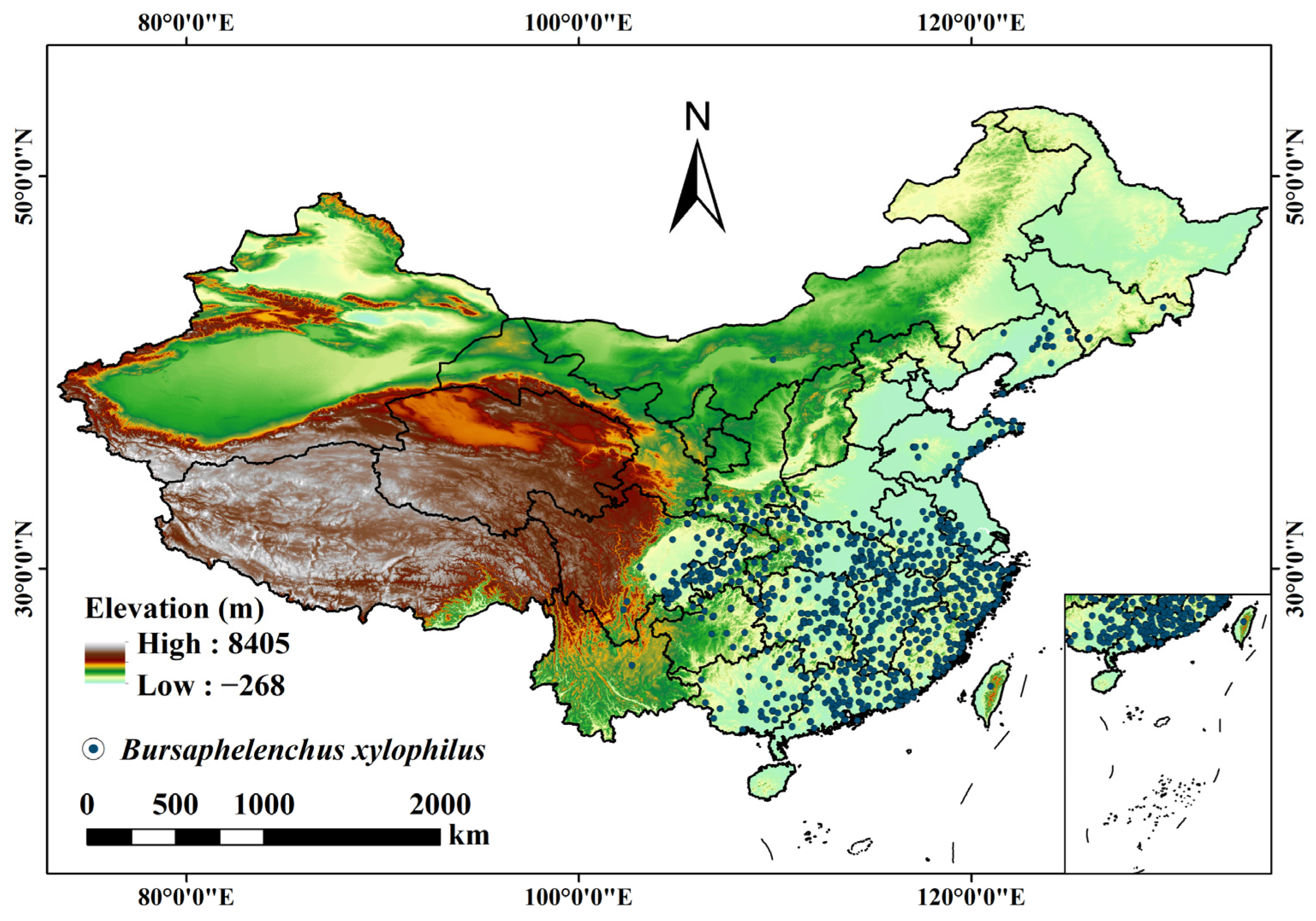
2.1. Data

To generate the occurrence records of B. xylophilus used in the modeling, we collected data from multiple sources, specifically the following: (1) information regarding endemic regions affected by B. xylophilus was obtained from the National Forestry and Grassland Administration (http://www.forestry.gov.cn, accessed on 2 June 2024); (2) book materials and online references (CNKI, https://www.cnki.net, accessed on 20 May 2024; WOS, https://www.webofscience.com/wos, accessed on 19 May 2024) [25,26]; and (3) two online public databases, the Global Biodiversity Information Facility (GBIF) (https://doi.org/10.15468/dl.uvs3yu, accessed on 18 May 2024) and an iNaturalist (https://www.inaturalist.org, accessed on 20 May 2024). For available record locations without specific latitude and longitude coordinates, we instead used Google Earth software (http://ditu.google.cn, accessed on 3 June 2024) to obtain this information. Ultimately, through these sources, a total of 1385 occurrence points were collected for this study (Figure 1). These records provided the necessary database for modeling.
In order to prevent model overfitting, the “ENMTools” package was employed to guarantee the quality of the dataset utilized for model construction and to minimize potential biases in spatial clustering due to data duplication, thereby enhancing the accuracy and reliability of the model [27]. The tool automatically identifies the cell size of the environmental factor grid and eliminates redundant data within the same grid, which in this study was set to 2.5 arcmin (~21 km2 at the equator). This approach is rapid and effective, and the results of the analysis are more meaningful. Consequently, the resulting occurrence records are necessarily smaller than the actual distribution area. Ultimately, 963 occurrence data points for B. xylophilus were retained for the construction of the MaxEnt model.
In this study, in order to analyze and predict the potential distribution area of B. xylophilus, we initially selected 31 environmental variables that may affect the distribution of B. xylophilus (Table 1). These variables cover a wide range of aspects, including bioclimatic, topographic, normalized difference vegetation index, ultraviolet radiation, and human activities [28]. Climate data at a resolution of 2.5 arcmin from the 1970s to 2000s were downloaded from WorldClim version 2.1 for the current period. Future climate data for the 2050s and 2070s were simulated under four shared socioeconomic pathways (SSPs) using the BCC-CSM2-MR global circulation model. Elevation data at 2.5 arcmin resolution were downloaded from WorldClim, and slope and aspect were extracted using ArcGIS Map software (version 10.8.1). We downloaded the normalized difference vegetation index (NDVI) data from the Center for Resource and Environmental Sciences and data from the Chinese Academy of Sciences (https://www.resdc.cn/, accessed on 19 January 2024). In addition, we have downloaded ultraviolet radiation data (https://www.ufz.de/gluv/index.php?en=32367, accessed on 19 January 2024). Human activity data were downloaded from the Socioeconomic Data and Applications Center (https://sedac.ciesin.columbia.edu, accessed on 15 January 2024), including the global human influence index and global human footprint. Finally, we used the “Resample” and “Extract” tools in the ArcGIS Map software to standardize the 31 environmental variables into a consistent format for subsequent analysis and modeling [29]. These data provide a comprehensive environmental background for studying the distribution of B. xylophilus in China, helping to understand the relationship between the species and its environment and to predict the possible effects of future climate change on the distribution of the species.
The selection and treatment of environmental variables is a crucial step when constructing a species distribution model, as the interconnections between variables may lead to autocorrelation and multicollinearity problems, which can reduce the predictive accuracy of the model [30]. To address these issues, we first assessed the contribution of the 31 environmental variables in the MaxEnt model using the Jackknife method, which identifies the variables that contribute most to the model predictions. Subsequently, a Pearson correlation analysis was conducted utilizing the “ENMTools” package (version 1.1.3) within the R platform (Figure S1). Environmental variables with correlation coefficients of |r| ≤ 0.9 were selected for modeling to avoid multicollinearity issues. When the correlation coefficient |r| > 0.9 between two environmental variables was observed, the variable with the higher contribution was chosen for inclusion in the model. This implies that in the case of highly correlated variables, only those that contribute the most to the model are retained. Through the aforementioned steps, 13 bioclimatic factors were ultimately incorporated into the MaxEnt model (Figure 2). These variables were deemed to be the most crucial and mutually independent environmental factors in the model, thereby enhancing the predictive accuracy and reliability of the model.

2.2. Evaluation and Validation of MaxEnt Model

Regularized multipliers (RMs) and feature combinations (FCs) serve as crucial parameters within the MaxEnt model, and optimizing these parameters can substantially enhance the model’s accuracy [31]. The RMs and FCs parameters were optimally tuned using the “ENMeval” package in the R software (version 4.3.3). Feature combinations encompass 5 feature types, namely L (linear features), Q (quadratic features), P (product features), T (threshold features), and H (hinge features). Initially, RMs were configured from 0 to 4 at intervals of 0.5 based on the preserved distribution data and environmental variables. Additionally, 6 FCs were designated to identify the optimal parameter combinations: L, LQ, H, LQH, LQHP, and LQHPT. Subsequently, 48 models incorporating various RM and FC combinations were constructed, and the model with the lowest delta AICc value among the feature combinations was selected as the optimal model (Figure S2). Finally, under natural environmental variable conditions, RMs were set to 0.5 with the FCs designated as “LQHP” (Figure S2A). Under conditions incorporating both natural environment variables and human activities, RMs were set to 1 with the FCs specified as “LQHPT” (Figure S2B). The additional parameter settings for the optimal model were as follows: 25% of the distribution points for each species were selected as the test set, while 75% were used for training. The maximum number of iterations was set to 5000, the maximum number of background points was limited to 10,000, and the repetitions were carried out 10 times. The closer the test omission rate is to the theoretical omission rate, the more accurate the model construction [32].
In ecological and environmental science research, the area under the curve (AUC) of the receiver operating characteristic curve (ROC) is an important metric for assessing the accuracy and predictive performance of modeling results [33]. The generalization ability of the model can be assessed by comparing the AUC values of the training and test sets and ensures that the model performs well on the training data and accurately predicts new and unseen data [34]. The AUC value determines the accuracy of the model, which ranges from 0 to 1. The larger the AUC value, the higher the accuracy of the model prediction. AUC values below 0.6 indicate a failure of the model performance, rendering the predictions unreliable. Values between 0.6 and 0.7 are considered poor, between 0.7 and 0.8 are considered fair, between 0.8 and 0.9 are considered good, and those above 0.9 are considered excellent. These values help to ensure the reliability and applicability of the findings.

2.3. Changes in the Potential Distribution Areas of B. xylophilus

The impact of natural environmental factors and human activities on the geospatial distribution pattern of B. xylophilus was investigated by developing three distinct models: (1) prediction of natural environmental factors (including bioclimate + topography + ultraviolet radiation + the normalized difference vegetation index) under the current climate model; (2) prediction of natural environmental factors (including bioclimate + topography + ultraviolet radiation + the normalized difference vegetation index) + human activity (including global human footprint + global human influence index) under the current climate model; and (3) prediction of natural environmental factors (including future bioclimate + topography + ultraviolet radiation + the normalized difference vegetation index) under the future climate model. Among them, model (1) and model (2) are based on current climate model projections, while model (3) is based on future climate model projections. Models (1) and (2) were employed to assess the influence of anthropogenic factors on the suitability of habitat for B. xylophilus, while models (1) and (3) were utilized to examine the potential effect of climate change on the suitability of habitat for B. xylophilus.
The average of the optimal MaxEnt model run through 10 repetitions was utilized as the final result, which was then evaluated based on the logistic value of the probability of species presence (P). The final results were converted to raster form and visualized using ArcGIS Map software, and the proportion of area in each suitable habitat was calculated. For comparison, the same thresholds were used for categorization in both the current and future climate models [35]. The suitability results for B. xylophilus were classified into two categories based on the natural breaks (Jenks) method in the ArcGIS Map software: unsuitable habitat (P < 0.172121) and suitable habitat (P ≥ 0.172121).

2.4. Change in Potential Distribution Center Shift under Future Climate Scenarios

We applied the “Centroid Changes (Lines)” tool in SDMToolbox v2.6 to identify potential geographic distribution centers in areas of high probability of species presence in each time period. The locations of potential distribution centers were compared across time and under different carbon emission scenarios. This helps to understand how the distribution of species changes in response to different climate change scenarios [36]. In addition, connecting the calculated potential distribution center points for different time periods represents the route of spatial change in the main suitable growing areas for B. xylophilus under future climate conditions.

2.5. Dynamics of Potential Distribution Areas of B. xylophilus under Future Climate Scenarios

We applied the “Distribution Changes between Species Distribution Models (SDMs)” function in SDMToolbox v2.6 to create binary maps with a threshold value of 0.172121, and the binary maps of each category in different future climate change scenarios were compared with the current climate scenarios to assess the future changes in the distribution of B. xylophilus [37]. Four results were obtained: “Expansion” (species range increases), “No occupancy” (species has no distribution under the new scenario), “Unchanged” (species range remains unchanged), and “Contraction” (species range decreases). In addition, we analyzed the extent of future climate change impacts on B. xylophilus in China using multivariate environmental similarity surfaces (MESSs) [38]. Environmental variables from contemporary potentially suitable areas were used as the reference layer to calculate the similarity between future climate conditions and the current one. The S value reflects the degree of similarity between the climate conditions at a point and the climate conditions in the reference layer during a given period. Negative values indicate that at least one of the environmental variables at the point has a value outside the range of the corresponding value in the reference layer, which is referred to as a climate anomaly, while a maximum value of 100 indicates that the climate at the point is completely normal. This operation is realized by running the “density.tools.Novel” tool in the “maxent.jar” file in the command window, and the ASCII file exported from the model was imported into ArcGIS Map 10.8.1 software for drawing.

2.6. Niche Dynamics Analyses

We conducted ecological niche quantification and overlap analyses using the “ecospat” software package (version 4.0.0) to explore climatic ecological niche changes between the ranges of B. xylophilus under contemporary and future climate scenarios [39]. Firstly, the presence and non-presence areas of B. xylophilus were binarised using ArcGIS Map software, with presence marked as 1 and non-presence marked as 0. Then, relevant environmental variables were extracted from each occurrence record. Subsequently, Schoener’s D index was employed to quantify the degree of overlap between ecological niches across climate scenarios, with values ranging from 0 (indicating no overlap) to 1 (representing complete overlap).

3. Results

3.1. Model Accuracy and Evaluation

The AUC values were applied to assess the accuracy of the optimized MaxEnt model in the prediction of species distributions. The results of this study showed that under contemporary climatic conditions, the average training AUC value of 10 repetitions of natural environmental variables was 0.9338, and the average testing AUC was 0.9285, while the average training AUC value of the model for the coexistence of natural environmental variables and human activities was 0.9500 and the average testing AUC value was 0.9465, which suggests that human activities may play an important role in predicting the results of the potential distributional areas of B. xylophilus potential distribution areas. In addition, the mean training AUC values and mean test AUC values for the different future carbon emission scenarios under the four climate change scenarios were greater than 0.9 (Table 2). This indicates that the optimized MaxEnt model is more accurate and precise and confirms the stability of the model’s robustness and generalization ability.

3.2. Main Environmental Variables Affecting Distribution of B. xylophilus

In this study, the effect of each variable on the geographic distribution of B. xylophilus was assessed using MaxEnt model outputs and Jackknife methods. This study found that the potential geographic distribution of B. xylophilus in the presence of only natural environmental factors was influenced by precipitation in the driest month (Bio14, 57.9%), annual precipitation (Bio12, 13.7%), elevation (Bio20, 10.6%), and the normalized difference vegetation index (Bio21, 6.2%), with a cumulative contribution of 88.4% (Figure 2). The main variables affecting the potential geographic distribution of B. xylophilus under a combination of natural environmental and human activities were precipitation in the driest month (Bio14, 44%), global human footprint (Bio30, 30.6%), and annual precipitation (Bio12, 7.1%), with a cumulative contribution of 81.7%. The variables with the largest changes in contribution were Bio14 (13.9% decrease), Bio12 (6.6% decrease), Bio20 (7.2% decrease), and Bio21 (4.4% increase) (Figure 2). This indicates that precipitation, the normalized difference vegetation index, elevation, and human activities are the main factors influencing the distribution of B. xylophilus.

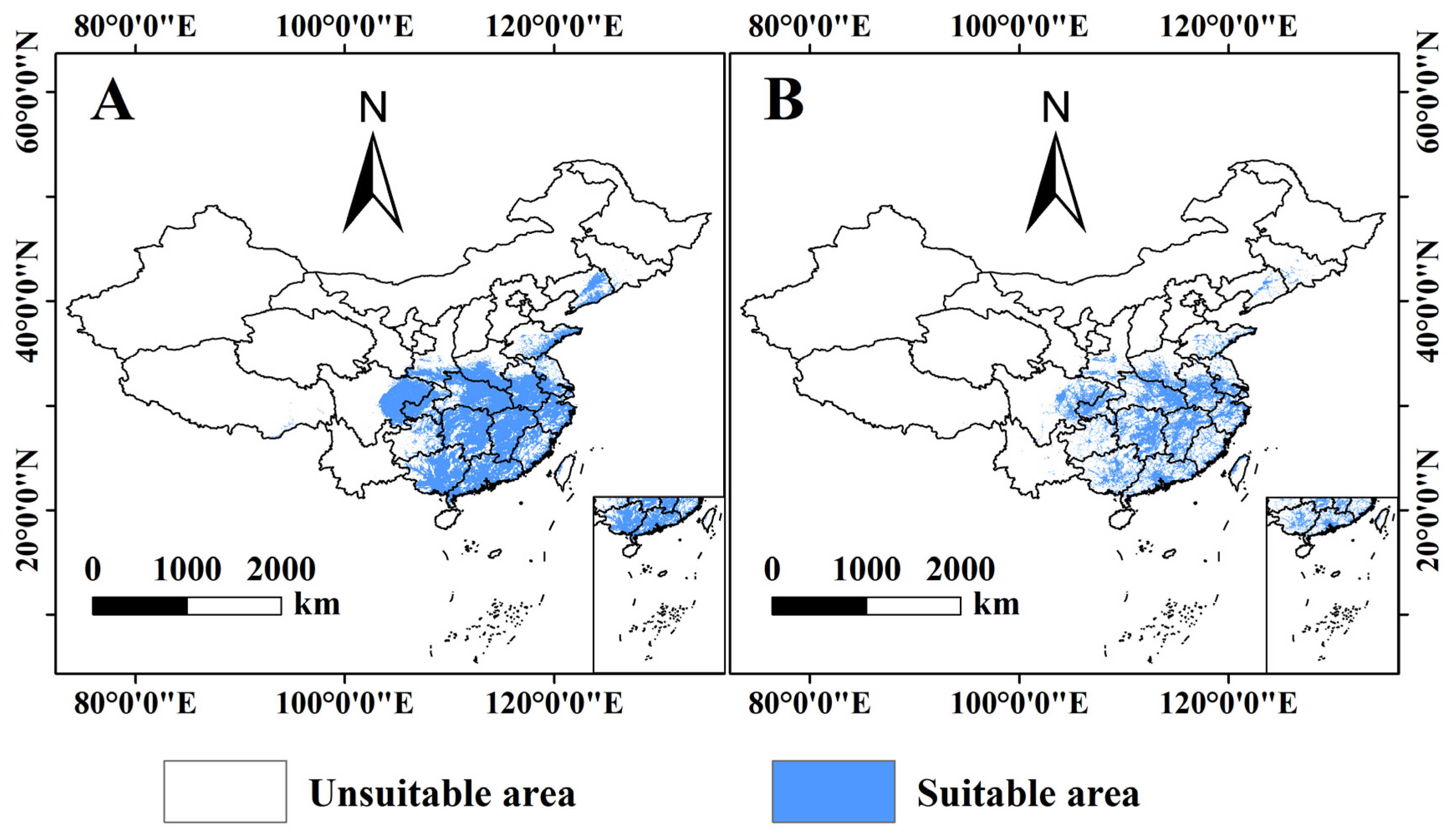
3.3. Prediction of the Potential Distribution of B. xylophilus under Climate and Human Interference in the Current

The MaxEnt model was employed to predict the spatial extent and habitat of B. xylophilus with and without anthropogenic disturbance (Figure 3), and the results showed that it was mainly distributed in central and southeastern China, which was similar to the actual occurrence area, indicating that the optimized MaxEnt model was able to simulate the potential distribution area of B. xylophilus well. Under the influence of natural environmental conditions, the occurrence areas of B. xylophilus were mainly concentrated in Liaoning, Shandong, Zhejiang, Anhui, Jiangsu, Shaanxi, Henan, Hubei, Hunan, Guangdong, Fujian, Chongqing, Sichuan, and Guangxi (Figure 3A). The suitable habitat covered an area of 138.58 × 10⁴ km2, representing 14.59% of China’s total land area (Table S1).
Taking into account human activities, the combined suitable habitat area for B. xylophilus in China was 80.13 × 10⁴ km2, making up 8.44% of China’s total land area. Conversely, unsuitable habitat covered 869.23 × 10⁴ km2, comprising 91.56% of China’s total area (Figure 3B). Compared with the area affected by natural environmental factors alone, there was a decrease of 42.18%, and the total area of suitable habitat for B. xylophilus decreased by 58.45 × 10⁴ km2, which represents 6.16% of China’s total land area (Table S1), indicating that human activities have reduced the area of suitable habitat for B. xylophilus.

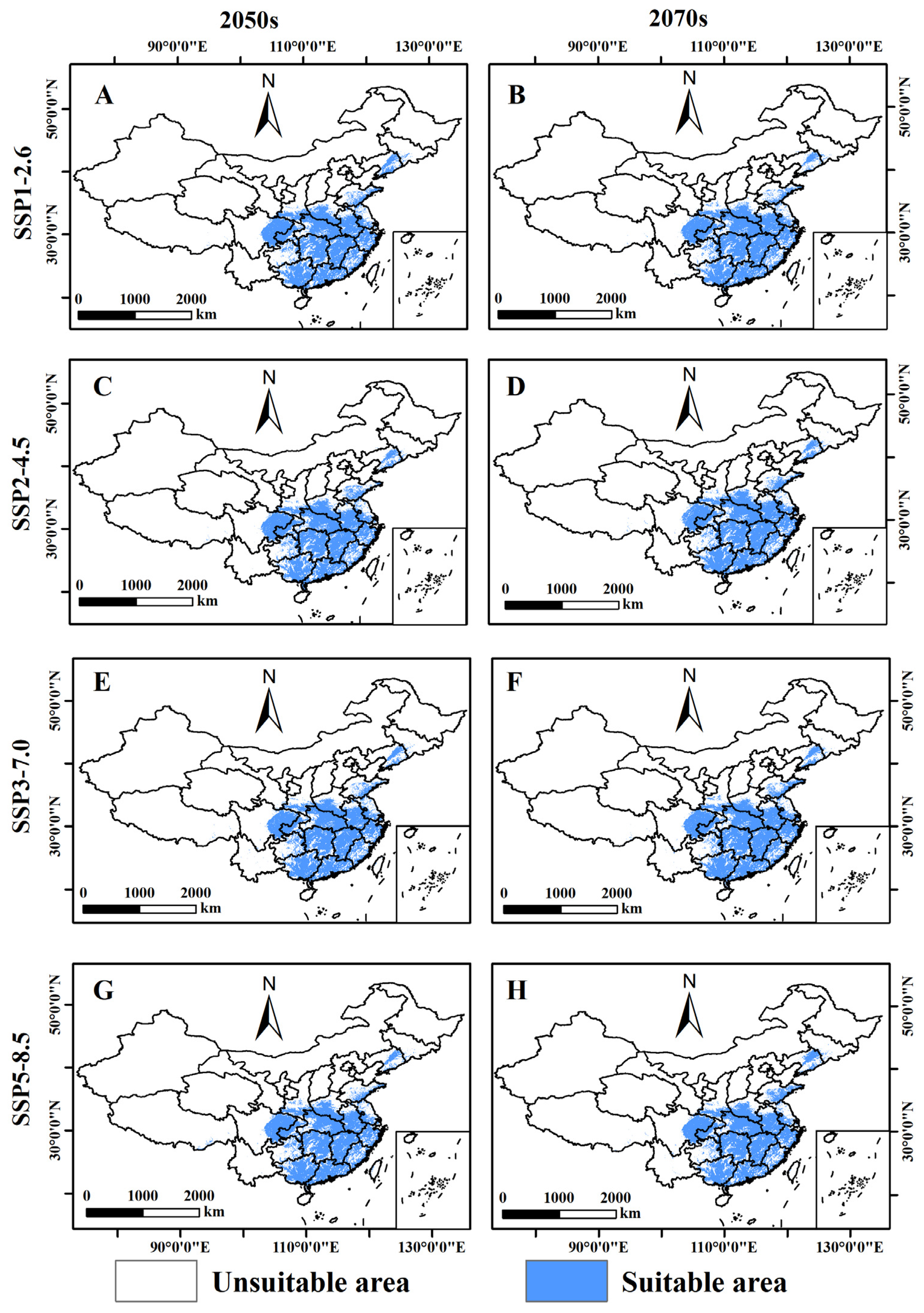
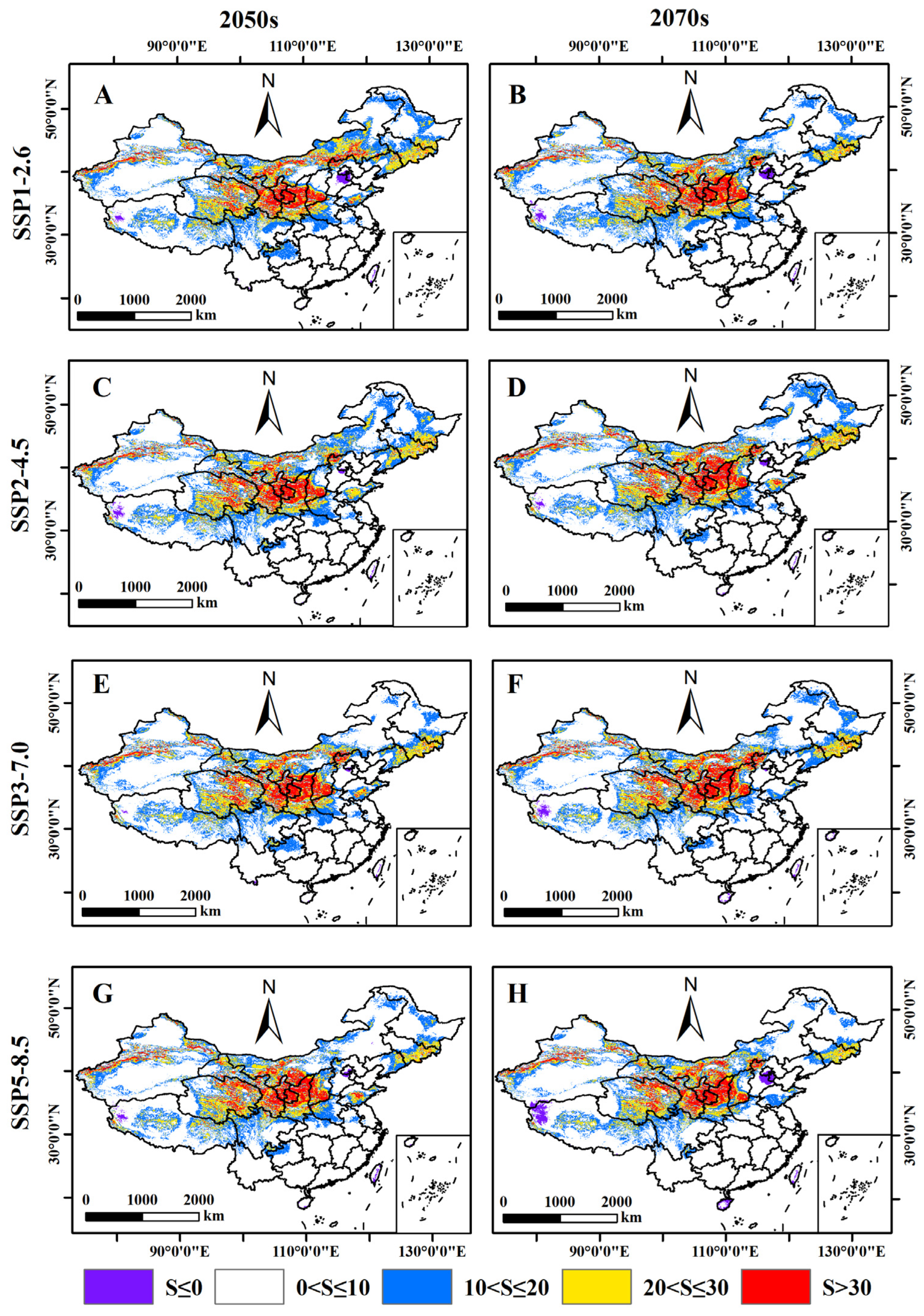
3.4. Prediction of the Potential Distribution of B. xylophilus under Different Climate Scenarios in the Future

In the context of climate change, the projected suitable ranges of B. xylophilus were based on future climate change scenarios with different common socioeconomic pathways and representative concentration pathways. The results showed that under different future climate scenarios, the range of suitable habitats for B. xylophilus was generally consistent with the current climate scenario and was mainly distributed in northeast, central and southeastern China, including Liaoning, Shandong, Zhejiang, Anhui, Jiangsu, Shaanxi, Henan, Hubei, Hunan, Guangdong, Fujian, Chongqing, Sichuan and Guangxi (Figure 4). Under the future climate scenarios, the estimated area of suitable habitat for B. xylophilus ranges from 137.87 × 10⁴ km2 to 141.55 × 10⁴ km2, accounting for 14.52% to 14.92% of China’s total area (Table S1). Among them, SSP3.0-7.0-2070s predicted the largest area of suitable habitat, followed by SSP5.0-8.5-2070s, while SSP1.0-2.6-2050s predicted the smallest area of suitable habitat. Over time, the area of suitable habitat for B. xylophilus showed a decreasing and then increasing trend in the low greenhouse gas emission scenario (SSP1.0-2.6, SSP2.0-4.5) and the medium greenhouse gas emission scenario (SSP3.0-7.0), i.e., the area of suitable habitat decreased in the 2050s and increased in the 2070s. However, only the SSP5.0-8.5 scenario shows a continuous increase (Table S1).

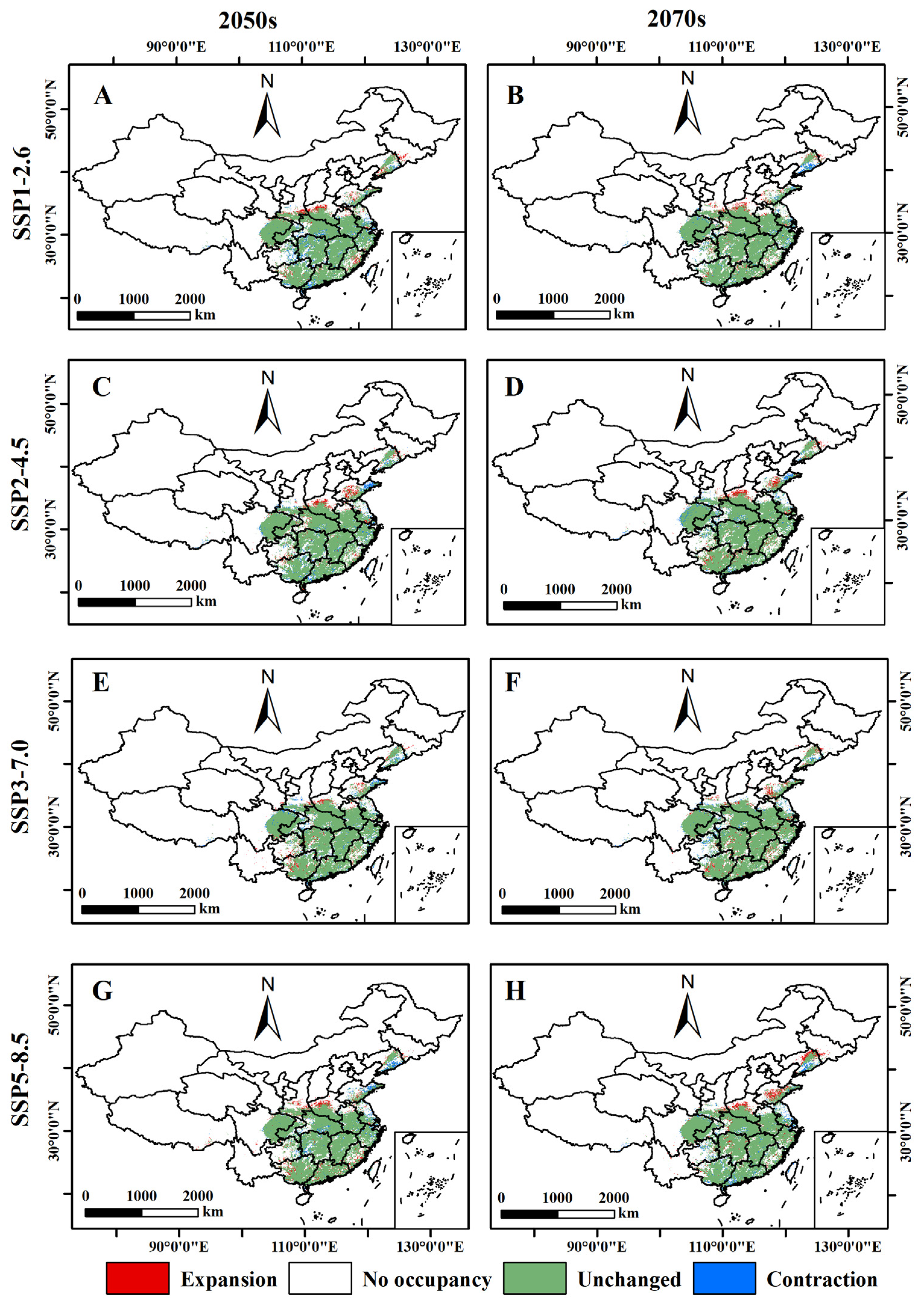
3.5. Relative Changes in the Potential Distribution Area of B. xylophilus under Future Climate Scenarios

Relative changes in the potential distribution of B. xylophilus were derived by comparing differences in current and future distribution areas (Figure 5 and Figure 6). The results showed that under future climate scenarios, the expansion area ranged from 18.16 × 10⁴ km2 to 29.82 × 10⁴ km2, and the contraction area ranged from 6.71 × 10⁴ km2 to 14.39 × 10⁴ km2 (Table S2). The expansion is primarily observed in Liaoning, Jilin, Shandong, Henan, Hubei, Guangxi, Guangdong, Guizhou, Jiangxi, Jiangsu, Anhui, Shaanxi, and Fujian. Conversely, the contraction area is predominantly found in Guangxi, Guangdong, Guizhou, Jiangxi, Fujian, Jiangsu, Shandong, Jilin, Xizang, and Taiwan Island (Figure 5). Among them, the largest expansion area was predicted for the high greenhouse gas (GHG) emission scenario SSP5.0-8.5-2070s, followed by SSP3.0-7.0-2070s, while the smallest expansion area was predicted for SSP1.0-2.6-2070s, which was development-pattern- and climate-change-dependent. Whereas the largest contraction area is in the low greenhouse gas (GHG) emission scenario (SSP1.0-2.6-2050s), the smallest is in the medium greenhouse gas (GHG) emission scenario (SSP3.0-7.0-2070s). Furthermore, under future climate scenarios, Inner Mongolia, Shanxi, Ningxia Hui Autonomous Region, Gansu, Qinghai, and Shaanxi exhibit a high degree of similarity with the climatic conditions of their origins (Figure 6), indicating that the climatic zones of the potential distribution area of B. xylophilus differ significantly from the current climate reference layer (Table S3).

3.6. Potential Distribution Center Shifts of B. xylophilus under Different Scenarios in the Future

We applied the “Centroid Changes (Lines)” tool to compare changes in the center of distribution of B. xylophilus under different carbon emission scenarios, which allowed us to assess the potential impacts of different emission reduction strategies on the movement routes and ecosystem stability of B. xylophilus. The current distribution center of B. xylophilus is located in Hubei Province at 113.18° N, 31.60° E (Figure 7 and Table 3). In the SSP1.0-2.6 pathway, the distribution center in the 2050s is located at 31.53° N, 113.49° E, and that in the 2070s is located at 32.35° N, 114.13° E, with the distribution center shifting 122.58 km to the northeast. In the SSP2.0-4.5 pathway, the distribution center was located at 31.71° N, 113.63° E in the 2050s and 31.75° N, 113.05° E in the 2070s, shifting the center of distribution by 20.86 km to the northwest. The distribution center in the SSP3.0-7.0 pathway was located at 31.63° N, 113.30° E in the 2050s and 31.55° N, 113.13° E in the 2070s and moved to the southwest by 7.20 km. In the SSP5.0-8.5 pathway, the distribution center for B. xylophilus was located at 31.87° N, 113.36° E in the 2050s and at 31.55° N, 113.40° E in the 2070s, with a southeast move of 21.02 km. As time goes on, the distribution center of B. xylophilus remained relatively stable between time points, suggesting that the MaxEnt model performs well in predicting the stability of the potential future range of the species, implying that the model’s selection and trade-offs of environmental variables were accurate (Figure 7 and Table 3).

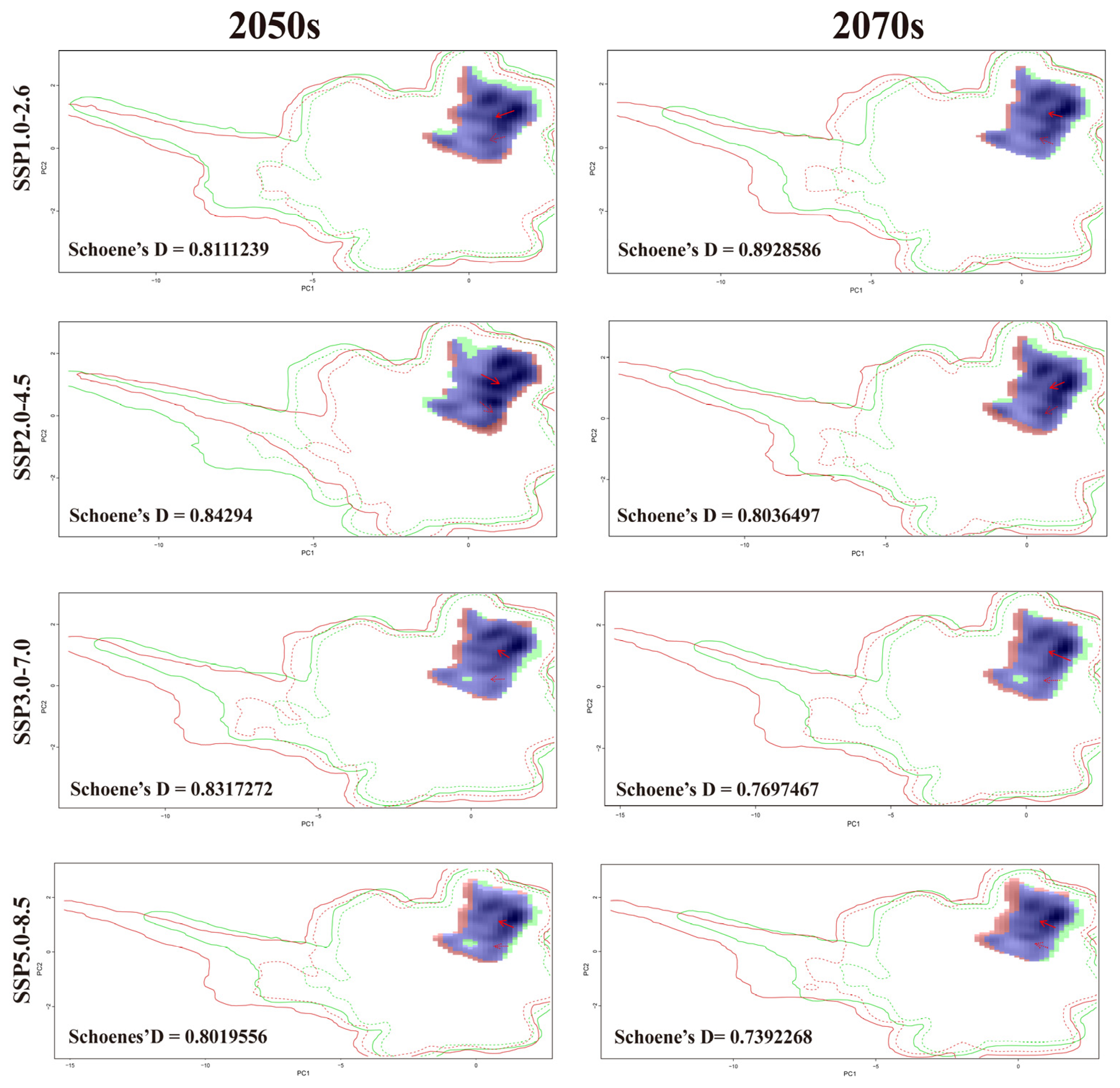
3.7. Niche Dynamics of B. xylophilus

The ecological niche similarity of B. xylophilus was analyzed under different climatic scenarios using ecological niche overlap (Figure 8). The Schoene’s D index ranged from 0.74 (current vs. SSP5.0-8.5-2070s) to 0.89 (current vs. SSP1.0-2.6-2070s). The higher overlap values indicate that the ecological niche of B. xylophilus is highly similar under different climate scenarios. This implies that despite future changes in climatic conditions, the ecological needs and adaptations of B. xylophilus remain largely consistent with current climatic variables and may not change significantly in its future range because it is able to adapt to these changes.

4. Discussion

The accuracy of ecological niche model prediction results depends on the selection of input data and adjustment of model parameters, both of which directly affect the output of the results [40,41]. In this experiment, we used more distribution point data than online books and public online databases and obtained the most recent distribution point data through the National Forestry and Grassland Administration (2024, NFGA) and the literature [25,26], which improved the accuracy and timeliness of the study. We also considered a variety of environmental factors, including climate change, terrain, ultraviolet radiation, NDVI, elevation, and human activities, which are considered to be key factors influencing the distribution and dynamics of B. xylostella. In addition, in order to prevent model overfitting, the MaxEnt model parameter was adjusted in this study, which helped to improve the accuracy and precision of prediction. The results of this study pointed out that all average AUC values exceeded 0.92, indicating the high predictive reliability of the model and the reliability of the findings, which is crucial for the development of science-based management strategies.
In this study, the potentially suitable habitats of B. xylophilus were found to be limited by Bio14, Bio12, Bio20, and Bio21 under the influence of no anthropogenic disturbance through the combined analysis of the contribution rate, the sequence importance value, and the Jackknife method, which indicates that the combined effect of humid and thermal conditions plays an important role in the potential distribution of B. xylophilus [42,43]. With climate change, there will be a gradual decrease in precipitation in the future and a decrease in water content in the soil, thus exacerbating drought stress. Changes in temperature and precipitation patterns due to climate change may have significant impacts on the species. Global warming may cause species to expand their ranges to higher latitudes or higher altitudes, while changes in precipitation patterns may affect species’ food chains and habitats [44]. Thus, instability in precipitation and temperature may threaten the distribution of B. xylophilus, leading to changes in their range and thus spreading to form new distribution patterns [45]. With the involvement of human activities, the global human footprint (Bio30) and the global human influence index (Bio31) are important human factors influencing the distribution of B. xylophilus. Expression of agricultural work, road construction, and urbanization can all lead to fragmentation of natural habitats, which in turn reduces areas suitable for B. xylophilus survival.
The actual distribution of B. xylophilus and the potential distribution area predicted by the model are clustered in northern and central China. These areas have suitable geo-climatic conditions for B. xylophilus growth, providing a favorable environment for the survival, reproduction, and spread of B. xylophilus [46]. In addition, the transmission of B. xylophilus is mainly dependent on its insect vectors, Monochamus alternatus and Monochamus saltuarius. The larvae of these insects bore holes within the trunks of trees to form channels where B. xylophilus is usually found in the woody parts of pine trees. As the larvae of the family Cerambycidae develop within the pine tree, they may carry B. xylophilus, and when they develop into adults, they burrow out of the pine tree. Cerambycidae insects may transmit B. xylophilus to healthy pines as they search for new pines in which to lay their eggs [47,48]. Therefore, the range and number of these insect vectors play a key role in the spread of pine nematode dispersal. The climatic conditions in central and northern provide favorable conditions for the growth of pine trees, as well as suitable environments for the reproduction and activities of Cerambycidae [49]. These factors work together to make southern, central, and northeastern China high-risk areas for the spread and propagation of the PWD.
Climate change has altered the phenology and geographical distribution of the B. xylophilus, resulting in expansion and contraction of its range [50]. The results show that the expansion areas occur mainly in southern, central, and northeastern China, especially in Liaoning, Jilin, Shandong, Henan, Fujian, and Guangdong. These areas may become more suitable for the survival and reproduction of B. xylophilus due to changes in temperature and precipitation patterns caused by climate change. On the contrary, the contraction areas of B. xylophilus mainly occurred in Guizhou, Jiangsu, and Liaoning, which may be due to environmental conditions that are no longer suitable for B. xylophilus survival due to climate change [51]. Under the low–medium carbon greenhouse gas (GHG) emission scenarios (SSP1.0-2.6 and SSP2.0-4.5), the contracted area of B. xylophilus was larger than the expanded area, suggesting that suitable habitats for B. xylophilus will be continuously lost with climate change. However, under the medium-to-high carbon greenhouse gas (GHG) emission scenarios (SSP3.0-7.0 and SSP5.0-8.5), the contracted area of B. xylophilus was smaller than the expanded area, which may indicate that B. xylophilus is less dependent on its current habitat and is able to adapt to a wider range of environmental conditions [52]. Similarly, it has been suggested that slight changes in the potential distribution of species as a result of climate change may be a consequence of the occurrence of their ecological amplitude and ecological niche width [53]. In this study, the ecological niche overlap analysis revealed that the ecological niche overlap of B. xylophilus was greater than 0.74 under different climatic scenarios, which indicates that B. xylophilus has a high ecological niche width and adaptability to maintain its ecological niche under different climatic conditions. In addition, the suitability areas of B. xylophilus did not change significantly under future climate change, which may imply that B. xylophilus has a strong adaptive capacity and can maintain its distribution range normally under the background of climate change.
Changes in temperature and precipitation patterns due to climate change can affect the geographic distribution of B. xylophilus, leading to a shift in its range center. This shift may occur towards higher or lower latitudes, depending on the different shared socioeconomic pathways (SSP) scenarios, which model the extent and rate of climate change [54]. Under the SSP1.0-2.6 and SSP2.0-4.5 scenarios, the B. xylophilus moves to higher latitudes, possibly because projected climate change under the low greenhouse gas (GHG) emissions scenario results in more favorable temperature and precipitation conditions at higher latitudes. In contrast, B. xylophilus migration to lower latitudes under the SSP3.0-7.0 and SSP5.0-8.5 scenarios may be due to the degradation of suitable areas at lower latitudes as a result of projected climate change under the medium–high greenhouse gas (GHG) emissions scenarios, forcing the species to search for new suitable habitats [55]. It is worth noting that migration to lower latitudes may be relative and does not necessarily mean that climatic conditions at lower latitudes become more favorable, but may simply be due to the degradation of suitable areas at higher latitudes [56]. In addition, geographical anomalies may also cause species to migrate to lower latitudes, suggesting that changes in species’ distributions may not only be due to climate change but may also be influenced by other factors, such as human activities that help certain species to overcome natural barriers and thus expand their ranges.
From the results of this study, we found that B. xylophilus is at risk of spreading to the northeast (Liaoning and Jilin) and central regions (Henan and Shandong) in the future, and that failure to prevent and control it in time may lead to the death of a large number of pine trees, which constitutes an ecological disaster. To address this challenge, China has taken a series of comprehensive control measures [57], which include the following: 1. timely detection of outbreaks through quarantine and monitoring to prevent the spread of the disease; 2. removal of infected trees to reduce the source of transmission of the pathogen; 3. control of insect vectors that transmit the B. xylophilus; 4. utilization of trunk injection techniques to inject insecticides into the tree, which distributes the drug throughout the tree by transpiration to kill the nematode; and 5. adoption of the natural enemies of the nematode, such as predatory nematodes or other microorganisms, to control pine nematode populations. A combination of the above measures can effectively control the spread of B. xylophilus and protect forest resources [58]. Nevertheless, due to the complexity and rapid spread of B. xylophilus, control requires sustained efforts and interdisciplinary cooperation to meet the challenges posed by B. xylophilus and thus protect China’s forest resources and ecological balance [59,60].

5. Conclusions

In this study, an optimized MaxEnt model was used to assess the potential distribution area and dynamics of B. xylophilus in China based on references and the latest distribution data published by the National Forestry and Grassland Administration, and a variety of environmental factors, including climate change, terrain, vegetation, ultraviolet radiation, and human interference. The prediction results showed that temperature, precipitation, NDVI, elevation, and human activities were the key factors affecting the distribution of B. xylophilus. Under current climatic conditions, suitable habitat areas are mainly distributed in Liaoning, Shandong, Zhejiang, Anhui, Jiangsu, Shaanxi, Henan, Hubei, Hunan, Guangdong, Fujian, Chongqing, Sichuan and Guangxi. Between 2050 and 2070, the potential range area of B. xylophilus is at risk of spreading to the northeast, suggesting that focused monitoring in the northeast is needed to prevent B. xylophilus from damaging pines in the region. Furthermore, the high ecological niche similarity indicates that B. xylophilus will be able to locate similar habitats under future climatic conditions, which may facilitate its spread and ability to adapt to new environments. The results of this study will provide valuable references for the development of sustainable management strategies for agriculture and forestry in China under the challenge of climate change, which will help to reduce economic losses and promote the healthy and stable development of ecosystems.

Supplementary Materials

The following supporting information can be downloaded at https://www.mdpi.com/article/10.3390/f15071253/s1, Figure S1: Correlation among the 31 bioclimatic variables; Figure S2: Tuning parameters for Bursaphelenchus xylophilus in predicting potential distribution regions using the MaxEnt model. Table S1: Area of B. xylophilus under current (with and without human activity disturbance) and future climate scenarios; Table S2: Relative change in potential range size of B. xylophilus under different future climate scenarios; Table S3: Multivariate environmental similarity surfaces (MESS) affecting the distribution of B. xylophilus under future climate conditions.

Author Contributions

Conceptualization, L.Z.; methodology, L.Z.; software, L.Z.; validation, L.Z. and P.W.; formal analysis, L.Z.; investigation, P.W. and G.X.; resources, W.W.; data curation, P.W. and G.X.; writing—original draft preparation, L.Z.; writing—review and editing, L.Z.; visualization, L.Z. and P.W.; supervision, W.W.; project administration, W.W.; funding acquisition, P.W. and W.W. All authors have read and agreed to the published version of the manuscript.

Funding

This work was funded by the Natural Science Foundation of Hubei Province (No. 2024AFB254) and the National Natural Science Foundation of China (No. 31672327).

Data Availability Statement

The data in this study are available from the corresponding author.

Acknowledgments

We appreciate the constructive comments of the anonymous reviewers and processing editors and their help in revising the manuscript.

Conflicts of Interest

The authors declare no conflicts of interest.

References

  1. Sun, S.X.; Zhang, Y.; Huang, D.Z.; Wang, H.; Cao, Q.; Fan, P.X.; Yang, N.; Zheng, P.M.; Wang, R.Q. The effect of climate change on the richness distribution pattern of oaks (Quercus L.) in China. Sci. Total Environ. 2020, 744, e140786. [Google Scholar] [CrossRef] [PubMed]
  2. Wei, X.J.; Xu, D.P.; Zhuo, Z.H. Predicting the impact of climate change on the geographical distribution of Leafhopper, Cicadella viridis in China through the MaxEnt model. Insects 2023, 14, 586. [Google Scholar] [CrossRef] [PubMed]
  3. Dawson, T.P.; Jackson, S.T.; House, J.I.; Prentice, I.C.; Mace, G.M. Beyond predictions: Biodiversity conservation in a changing climate. Science 2011, 332, 53–58. [Google Scholar] [CrossRef] [PubMed]
  4. Urban, M.C. Accelerating extinction risk from climate change. Science 2015, 348, 571–573. [Google Scholar] [CrossRef] [PubMed]
  5. Pound, K.L.; Larson, C.A.; Passy, S.I.; Webb, T. Current distributions and future climate–driven changes in diatoms, insects and fish in U.S. streams. Global Ecol. Biogeogr. 2021, 30, 63–78. [Google Scholar] [CrossRef]
  6. Liu, T.; Liu, H.Y.; Wang, Y.J.; Yang, Y.X. Climate change impacts on the potential distribution pattern of Osphya (Coleoptera: Melandryidae), an old but small beetle group distributed in the Northern Hemisphere. Insects 2023, 14, 476. [Google Scholar] [CrossRef] [PubMed]
  7. Hardy, P.B.; Kinder, P.M.; Sparks, T.H.; Dennis, R.L.H. Elevation and habitats: The potential of sites at different altitudes to provide refuges for phytophagous insects during climatic fluctuations. J. Insect. Conserv. 2010, 14, 297–303. [Google Scholar] [CrossRef]
  8. Wu, Z.; Li, M.; Wang, B.; Tian, Y.; Quan, Y.; Liu, J. Analysis of factors related to forest fires in different forest ecosystems in China. Forests 2022, 13, 1021. [Google Scholar] [CrossRef]
  9. Sharma, A.; Jose, S.; Bohn, K.K.; Andreu, M.G. Effects of reproduction methods and overstory species composition on understory light availability in longleaf pine-slash pine ecosystems. For. Ecol. Manag. 2012, 284, 23–33. [Google Scholar] [CrossRef]
  10. Tuomola, J.; Gruffudd, H.; Ruosteenoja, K.; Hannunen, S. Could pine wood nematode (Bursaphelenchus xylophilus) cause pine wilt disease or even establish inside healthy trees in finland Now-Or ever? Forests 2021, 12, 1679. [Google Scholar] [CrossRef]
  11. Shi, L.; Wang, L.; Shi, X.; Luo, L.; Ye, J. Negative effects of free-living nematodes on the populations of Bursaphelenchus xylophilus in dead pine trees. Biol. Control 2022, 168, 104858. [Google Scholar] [CrossRef]
  12. Takai, K.; Soejima, T.; Suzuki, T.; Kawazu, K. Development of a water-soluble preparation of emamectin benzoate and its preventative effect against the wilting of pot-grown pine trees inoculated with the pine wood nematode, Bursaphelenchus xylophilus. Pest. Manag. Sci. 2001, 57, 463–466. [Google Scholar] [CrossRef] [PubMed]
  13. Hu, L.; Wu, X.; Ding, X.; Ye, J. Comparative transcriptomic analysis of candidate effectors to explore the infection and survival strategy of Bursaphelenchus xylophilus during different interaction stages with pine trees. BMC Plant Biol. 2021, 21, 224. [Google Scholar] [CrossRef] [PubMed]
  14. Zhang, X.L.; Qin, X.D.; Alvarez, F.; Chen, Z.N.; Wu, Z.J. Potential impact of land–use change on habitat quality in the distribution range of crocodile lizards in China. Ecol. Evol. 2022, 12, 9390. [Google Scholar] [CrossRef]
  15. Wang, D.; Cui, B.C.; Duan, S.S.; Chen, J.J.; Fan, H.; Lu, B.B.; Zheng, J.H. Moving north in China: The habitat of Pedicularis kansuensis in the context of climate change. Sci. Total Environ. 2019, 697, 133979. [Google Scholar] [CrossRef] [PubMed]
  16. Zhang, H.; Song, J.Y.; Zhao, H.X.; Li, M.; Han, W.H. Predicting the distribution of the invasive species Leptocybe invasa: Combining MaxEnt and geodetector models. Insects 2021, 12, 92. [Google Scholar] [CrossRef] [PubMed]
  17. Iannella, M.; Console, G.; Cerasoli, F.; De Simone, W.; D’Alessandro, P.; Biondi, M. A step towards SDMs: A “couple-and-weigh” framework based on accessible data for biodiversity conservation and landscape planning. Divers. Distrib. 2021, 27, 2412–2427. [Google Scholar] [CrossRef]
  18. Hadi Ahmad, M.; Abubakar, A.; Yusoff Ishak, M.; Shehu Danhassan, S.; Zhang, J.H.; Aiatalo, J.M. Modeling the influence of daily temperature and precipitation extreme indices on vegetation dynamics in Katsina State using statistical downscaling model (SDM). Ecol. Indic. 2023, 155, 110979. [Google Scholar] [CrossRef]
  19. Wang, Z.L.; Xu, D.P.; Liao, W.K.; Xu, Y.; Zhuo, Z.H. Predicting the current and future distributions of Frankliniella occidentalis (Pergande) based on the MaxEnt species distribution model. Insects 2023, 14, 458. [Google Scholar] [CrossRef]
  20. Harte, J.; Umemura, K.; Brush, M.; Chase, J. DynaMETE: A hybrid MaxEnt–plus–mechanism theory of dynamic macroecology. Ecol. Lett. 2021, 24, 935–949. [Google Scholar] [CrossRef]
  21. Guga, S.; Xu, J.; Riao, D.; Li, K.W.; Han, A.; Zhang, J.Q. Combining MaxEnt model and landscape pattern theory for analyzing interdecadal variation of sugarcane climate suitability in Guangxi, China. Ecol. Indic. 2021, 131, 108152. [Google Scholar] [CrossRef]
  22. Soliman, M.M.; Al-Khalaf, A.A.; El-Hawagry, M.S.A. Effects of climatic change on potential distribution of Spogostylum ocyale (Diptera: Bombyliidae) in the middle east using Maxent modelling. Insects 2023, 14, 120. [Google Scholar] [CrossRef] [PubMed]
  23. Lee, C.M.; Lee, D.S.; Kwon, T.S.; Athar, M.; Park, Y.S. Predicting the global distribution of Solenopsis geminata (Hymenoptera: Formicidae) under climate change using the MaxEnt model. Insects 2021, 12, 229. [Google Scholar] [CrossRef] [PubMed]
  24. Zheng, Y.X.; Chao, Y.; Matsushita, N.; Lian, C.L.; Geng, Q.F. Analysis of the distribution pattern of the ectomycorrhizal fungus Cenococcum geophilum under climate change using the optimized MaxEnt model. Ecol. Evol. 2023, 13, 10565. [Google Scholar] [CrossRef] [PubMed]
  25. Ouyang, X.; Chen, A.; Li, Y.; Han, X.; Lin, H. Predicting the potential distribution of pine wilt disease in china under climate change. Insects 2022, 13, 1147. [Google Scholar] [CrossRef] [PubMed]
  26. Xiao, Y.; Guo, Q.; Xie, N.; Yuan, G.; Liao, M.; Gui, Q.; Ding, G. Predicting the global potential distribution of Bursaphelenchus xylophilus using an ecological niche model: Expansion trend and the main driving factors. BMC Ecol Evol. 2024, 24, 48. [Google Scholar] [CrossRef] [PubMed]
  27. Warren, D.L.; Matzke, N.J.; Cardillo, M.; Baumgartner, J.B.; Beaumont, L.J.; Turelli, M.; Glor, R.E.; Huron, N.A.; Simoes, M.; Iglesias, T.L.; et al. ENMTools 1.0: An R package for comparative ecological biogeography. Ecography 2021, 44, 504–511. [Google Scholar] [CrossRef]
  28. Wu, T.W.; Lu, Y.X.; Fang, Y.J.; Xin, X.G.; Li, L.; Li, W.P.; Jie, W.H.; Zhang, J.; Liu, Y.M.; Zhang, L.; et al. The Beijing climate center climate system model (BCC-CSM): The main progress from CMIP5 to CMIP6. Geosci. Model Dev. 2019, 12, 1573–1600. [Google Scholar] [CrossRef]
  29. Li, D.X.; Li, Z.X.; Liu, Z.W.; Yang, Y.J.; Khoso, A.G.; Wang, L.; Liu, D.G. Climate change simulations revealed potentially drastic shifts in insect community structure and crop yields in China’s farmland. J. Pest Sci. 2022, 96, 1–15. [Google Scholar] [CrossRef]
  30. Phillips, S.J.; Anderson, R.P.; Schapire, R.E. Maximum entropy modeling of species geographic distributions. Ecol. Model. 2006, 190, 231–259. [Google Scholar] [CrossRef]
  31. Kaky, E.; Nolan, V.; Alatawi, A.; Gilbert, F. A comparison between ensemble and MaxEnt species distribution modelling approaches for conservation: A case study with Egyptian medicinal plants. Ecol. Inf. 2020, 60, 101150. [Google Scholar] [CrossRef]
  32. Maruthadurai, R.; Das, B.; Ramesh, R. Predicting the invasion risk of rugose spiraling Whitefly, Aleurodicus rugioperculatus, in India based on CMIP6 projections by MaxEnt. Pest Manag. Sci. 2023, 79, 295–305. [Google Scholar] [CrossRef] [PubMed]
  33. Yoon, S.; Lee, W.H. Assessing potential European areas of Pierce’s disease mediated by insect vectors by using spatial ensemble model. Front. Plant Sci. 2023, 14, 1209694. [Google Scholar] [CrossRef]
  34. Aidoo, O.F.; Souza, P.G.C.; Silva, R.S.; Santana, P.A.; Picanço, M.C.; Kyerematen, R.; Sètamou, M.; Ekesi, S.; Borgemeister, C. Climate-induced range shifts of invasive species (Diaphorina citri Kuwayama). Pest Manag. Sci. 2022, 78, 2534–2549. [Google Scholar] [CrossRef]
  35. Yang, S.L.; Wang, H.M.; Tong, J.P.; Bai, Y.; Alatalo, J.M.; Liu, G.; Fang, Z.; Zhang, F. Impacts of environment and human activity on grid-scale land cropping suitability and optimization of planting structure, measured based on the MaxEnt model. Sci. Total Environ. 2022, 836, 155356. [Google Scholar] [CrossRef] [PubMed]
  36. Gao, R.H.; Liu, L.; Zhao, L.J.; Cui, S.P. Potentially suitable geographical area for Monochamus alternatus under current and future climatic scenarios based on optimized MaxEnt model. Insects 2023, 14, 182. [Google Scholar] [CrossRef]
  37. Huang, M.Y.; Ge, X.Z.; Shi, H.L.; Tong, Y.G.; Shi, J. Prediction of current and future potential distributions of the Eucalyptus pest Leptocybe invasa (Hymenoptera: Eulophidae) in China using the CLIMEX model. Pest Manag. Sci. 2019, 75, 2958–2968. [Google Scholar] [CrossRef] [PubMed]
  38. Wang, B.X.; Hof, A.R.; Matson, K.D.; Langevelde, F.; Ma, C.S. Climate change, host plant availability, and irrigation shape future region–specific distributions of the Sitobion grain aphid complex. Pest Manag. Sci. 2023, 79, 2311–2324. [Google Scholar] [CrossRef]
  39. Liu, T.; Liu, H.; Li, Y.; Yang, Y. Staying on the current niche: Consensus model reveals the habitat loss of a critically endangered dragonfly Libellula angelina under climate changes. J Insect Conserv. 2024, 28, 483–499. [Google Scholar] [CrossRef]
  40. Ge, X.Z.; He, S.Y.; Zhu, C.Y.; Wang, T.; Xu, Z.C.; Zong, S.X. Projecting the current and future potential global distribution of Hyphantria cunea (Lepidoptera: Arctiidae) using CLIMEX. Pest Manag. Sci. 2019, 75, 160–169. [Google Scholar] [CrossRef]
  41. Gao, H.; Qian, Q.Q.; Liu, L.J.; Xu, D.P. Predicting the distribution of Sclerodermus sichuanensis (Hymenoptera: Bethylidae) under climate change in China. Insects 2023, 14, 475. [Google Scholar] [CrossRef] [PubMed]
  42. Zhao, M.Z.; Duan, Q.; Shen, X.Y.; Zhang, S.Y. Climate change influences the population density and suitable area of Hippotiscus dorsalis (Hemiptera: Pentatomidae) in China. Insects 2023, 14, 135. [Google Scholar] [CrossRef] [PubMed]
  43. Santana, P.A.; Kumar, L.; Da Silva, R.S.; Picanço, M.C. Global geographic distribution of Tuta absoluta as affected by climate change. J. Pest Sci. 2019, 92, 1373–1385. [Google Scholar] [CrossRef]
  44. Kumar, A.V.; Zimova, M.; Martin, T.E.; Mills, L.S. Contrasting seasonal effects of climate change influence density in a cold–adapted species. Global Change Biol. 2022, 28, 6228–6238. [Google Scholar] [CrossRef] [PubMed]
  45. Santana, P.A.; Kumar, L.; Da Silva, R.S.; Pereira, J.L.; Picanço, M.C. Assessing the impact of climate change on the worldwide distribution of Dalbulus maidis (DeLong) using MaxEnt. Pest Manag. Sci. 2019, 10, 2706–2715. [Google Scholar] [CrossRef] [PubMed]
  46. Mazziotta, A.; Lundström, J.; Forsell, N.; Moor, H.; Eggers, J.; Subramanian, N.; Aquilué, N.; Morán–Ordóñez, A.; Brotons, L.; Snäll, T. More future synergies and less trade–offs between forest ecosystem services with natural climate solutions instead of bioeconomy solutions. Global Change Biol. 2022, 28, 6333–6348. [Google Scholar] [CrossRef] [PubMed]
  47. Lee, B.; Yang, J.; Beckett, S.; Ren, Y. Preliminary trials of the ethanedinitrile fumigation of logs for eradication of Bursaphelenchus xylophilus and its vector insect Monochamus alternatus: C 2 N 2 fumigation of logs to eradicate B. xylophilus and its vector insect M. alternatus. Pest. Manag. Sci. 2017, 73, 1446–1452. [Google Scholar] [CrossRef]
  48. Wang, J.; Zhang, S.; Zheng, Y. Feeding preferences and responses of Monochamus saltuarius to volatile components of host pine trees. Insects 2022, 13, 888. [Google Scholar] [CrossRef] [PubMed]
  49. Meng, F.; Liu, Z.; Li, Y.; Zhang, X. Genes encoding potential molecular mimicry proteins as the specific targets for detecting Bursaphelenchus xylophilus in PCR and loop-mediated isothermal amplification assays. Front. Plant Sci. 2022, 13, 890949. [Google Scholar] [CrossRef]
  50. Wedegärtner, R.E.M.; Lembrechts, J.J.; Van der Wal, R.; Barros, A.; Chauvin, A.; Janssens, I.; Graae, B.J. Hiking trails shift plant species’ realized climatic niches and locally increase species richness. Divers. Distrib. 2022, 28, 1416–1429. [Google Scholar] [CrossRef]
  51. Haran, J.; Roques, A.; Bernard, A.; Robinet, C.; Roux, G. Altitudinal barrier to the spread of an invasive species: Could the pyrenean chain slow the natural spread of the pinewood nematode? PLoS ONE. 2015, 10, e0134126. [Google Scholar] [CrossRef] [PubMed]
  52. Spaak, J.W.; Carpentier, C.; De Laender, F.; Mayfield, M. Species richness increases fitness differences, but does not affect niche differences. Ecol. Lett. 2021, 24, 2611–2623. [Google Scholar] [CrossRef] [PubMed]
  53. Yin, X.; Jarvie, S.; Guo, W.; Deng, T.; Mao, L.; Zhang, M.; Chu, C.; Qian, H.; Svenning, J.; He, F.; et al. Niche overlap and divergence times support niche conservatism in eastern Asia-eastern north America disjunct plants. Global Ecol. Biogeogr. 2021, 30, 1990–2003. [Google Scholar] [CrossRef]
  54. Ling, P.Y.; Aguilar-Amuchastegui, N.; Baldwin-Cantello, W.; Rayden, T.; Gordon, J.; Dainton, S.; Bagwill, A.L.; Pacheco, P. Mapping global forest regeneration–an untapped potential to mitigate climate change and biodiversity loss. Environ. Res. Lett. 2023, 18, 54025. [Google Scholar] [CrossRef]
  55. Zhang, Z.X.; Kass, J.M.; Mammola, S.; Koizumi, I.; Li, X.C.; Tanaka, K.; Ikeda, K.; Suzuki, T.; Yokota, M.; Usio, N. Lineage-level distribution models lead to more realistic climate change predictions for a threatened crayfish. Divers. Distrib. 2021, 27, 684–695. [Google Scholar] [CrossRef]
  56. Jiang, K.; Teuling, A.J.; Chen, X.; Huang, N.; Wang, J.; Zhang, Z.; Gao, R.; Men, J.; Zhang, Z.; Wu, Y.; et al. Global land degradation hotspots based on multiple methods and indicators. Ecol. Indic. 2024, 158, 111462. [Google Scholar] [CrossRef]
  57. Zhou, X.; Chen, S.; Lu, F.; Guo, K.; Huang, L.; Su, X.; Chen, Y. Nematotoxicity of a Cyt–like protein toxin from Conidiobolus obscurus (entomophthoromycotina) on the pine wood nematode Bursaphelenchus xylophilus. Pest. Manag. Sci. 2021, 77, 686–692. [Google Scholar] [CrossRef]
  58. Shi, F.; Ge, S.; Hou, Z.; Xu, Y.; Tao, J.; Wu, H.; Zong, S. Species–specific primers for rapid detection of Monochamus saltuarius, an effective vector of Bursaphelenchus xylophilus in China. J. Appl. Entomol. 2022, 146, 636–647. [Google Scholar] [CrossRef]
  59. Park, C.G.; Son, J.; Lee, B.; Cho, J.H.; Ren, Y. Comparison of ethanedinitrile (C2N2) and metam sodium for control of Bursaphelenchus xylophilus (Nematoda: Aphelenchidae) and Monochamus alternatus (Coleoptera: Cerambycidae) in naturally infested logs at low temperatures. J. Econ. Entomol. 2014, 107, 2055–2060. [Google Scholar] [CrossRef]
  60. Gruffudd, H.R.; Schröder, T.; Jenkins, T.A.R.; Evans, H.F. Modelling pine wilt disease (PWD) for current and future climate scenarios as part of a pest risk analysis for pine wood nematode Bursaphelenchus xylophilus (Steiner and Buhrer) Nickle in Germany. J. Plant Dis. Prot. 2019, 126, 129–144. [Google Scholar] [CrossRef]
Figure 1. Occurrence records of B. xylophilus within China.
Forests 15 01253 g001
Figure 2. Contribution of 13 environmental variables after screening.
Forests 15 01253 g002
Figure 3. Distribution of suitable habitat for B. xylophilus without (A) and with (B) human activity under current climate models in China.
Forests 15 01253 g003
Figure 4. Suitable areas for B. xylophilus in China under different future climate scenarios. (A) SSP1.0-2.6-2050s; (B) SSP1.0-2.6-2070s; (C) SSP2.0-4.5-2050s; (D) SSP2.0-4.5-2070s; (E) SSP3.0-7.0-2050s; (F) SSP3.0-7.0-2070s; (G) SSP5.0-8.5-2050s; (H) SSP5.0-8.5-2070s.
Forests 15 01253 g004
Figure 5. Relative changes in B. xylophilus within China under different future climate scenarios. (A) SSP1.0-2.6-2050s; (B) SSP1.0-2.6-2070s; (C) SSP2.0-4.5-2050s; (D) SSP2.0-4.5-2070s; (E) SSP3.0-7.0-2050s; (F) SSP3.0-7.0-2070s; (G) SSP5.0-8.5-2050s; (H) SSP5.0-8.5-2070s.
Forests 15 01253 g005
Figure 6. MESS analysis for B. xylophilus under future climate scenarios in China. (A) SSP1.0-2.6-2050s; (B) SSP1.0-2.6-2070s; (C) SSP2.0-4.5-2050s; (D) SSP2.0-4.5-2070s; (E) SSP3.0-7.0-2050s; (F) SSP3.0-7.0-2070s; (G) SSP5.0-8.5-2050s; (H) SSP5.0-8.5-2070s.
Forests 15 01253 g006
Figure 7. (A) Moving trajectories of potential distribution center routes for B. xylophilus in China; (B) The B. xylophilus movement routes under different shared socio-economic path models; (C) SSP1.0-2.6; (D) SSP2.0-4.5; (E) SSP3.0-7.0; (F) SSP5.0-8.5.
Forests 15 01253 g007
Figure 8. Future analysis of B. xylophilus ecological niche dynamics under different climate scenarios. The blue areas show the stable habitats of B. xylophilus, the green areas show the habitats it will lose, and the pink areas show the habitats that are shifting. The red arrow shows the direction of niche migration for B. xylophilus in future climates. Solid and dashed lines connect the current and future distribution centers, with the dashed lines outlining the potential range of distribution changes.
Forests 15 01253 g008
Table 1. Screening of 31 environmental variables.
AbbreviationEnvironmental VariablesOperation (|r| > 0.9)
Bio1Annual mean temperature (°C)Retain
Bio2Mean diurnal range (°C)Retain
Bio3IsothermalityRetain
Bio4Temperature seasonalityRetain
Bio5Maximum temp of warmest month (°C)Eliminate
Bio6Minimum temp of coldest month (°C)Eliminate
Bio7Temperature annual range (°C)Eliminate
Bio8Mean temp of wettest quarter (°C)Eliminate
Bio9Mean temp of driest quarter (°C)Eliminate
Bio10Mean temp of warmest quarter (°C)Eliminate
Bio11Mean temp of coldest quarter (°C)Eliminate
Bio12Annual precipitation (mm)Retain
Bio13Precipitation of wettest month (mm)Eliminate
Bio14Precipitation of driest month (mm)Retain
Bio15Precipitation seasonality (mm)Retain
Bio16Precipitation of wettest quarter (mm)Eliminate
Bio17Precipitation of driest quarter (mm)Eliminate
Bio18Precipitation of warmest quarter (mm)Eliminate
Bio19Precipitation of coldest quarter (mm)Eliminate
Bio20Elevation (m)Retain
Bio21NDVIRetain
Bio22SlopeRetain
Bio23AspectRetain
Bio24Annual_mean_UV-BEliminate
Bio25UV-B_seasonalityEliminate
Bio26Mean_UV-B_of_highest_monthEliminate
Bio27Mean_UV-B_of_lowest_monthEliminate
Bio28Sum_of_UV-B_radiation_of_highest_quarterEliminate
Bio29Sum_of_UV-B_radiation_of_lowest_quarterEliminate
Bio30Global human footprintRetain
Bio31Global human influence indexRetain
Table 2. Model accuracy evaluation.
Shared Socioeconomic PathwaysTrain AUC (Avg)Test AUC (Avg)
Current-Environmental variables0.93380.9285
Current-Environmental variables + Human activity0.95000.9465
Future-SSP1.0-2.6 2040–20600.93450.9277
Future-SSP1.0-2.6 2060–20800.93380.9284
Future-SSP2.0-4.5 2040–20600.93490.9287
Future-SSP2.0-4.5 2060–20800.93420.9291
Future-SSP3.0-7.0 2040–20600.93570.9302
Future-SSP3.0-7.0 2060–20800.93240.9266
Future-SSP5.0-8.5 2040–20600.93510.9301
Future-SSP5.0-8.5 2060–20800.93510.9286
Table 3. Trends in longitude, latitude, and migration distance of B. xylophilus in different periods.
Shared Socioeconomic PathwaysLongitude (°E)Latitude (°N)Center Migration Distance (km)
Current113.1831.60-
Future-SSP1.0-2.6 2040–2060113.4931.5330.52
Future-SSP1.0-2.6 2060–2080114.1332.35122.58
Future-SSP2.0-4.5 2040–2060113.6331.7143.98
Future-SSP2.0-4.5 2060–2080113.0531.7520.86
Future-SSP3.0-7.0 2040–2060113.3031.6311.93
Future-SSP3.0-7.0 2060–2080113.1331.557.20
Future-SSP5.0-8.5 2040–2060113.3631.8734.76
Future-SSP5.0-8.5 2060–2080113.4031.5521.02
Disclaimer/Publisher’s Note: The statements, opinions and data contained in all publications are solely those of the individual author(s) and contributor(s) and not of MDPI and/or the editor(s). MDPI and/or the editor(s) disclaim responsibility for any injury to people or property resulting from any ideas, methods, instructions or products referred to in the content.

