


Estimation of Leaf Area Index for Dendrocalamus giganteus Based on Multi-Source Remote Sensing Data

 , ,
, ,  , ,
, ,
Abstract
1. Introduction
2. Materials and Methods
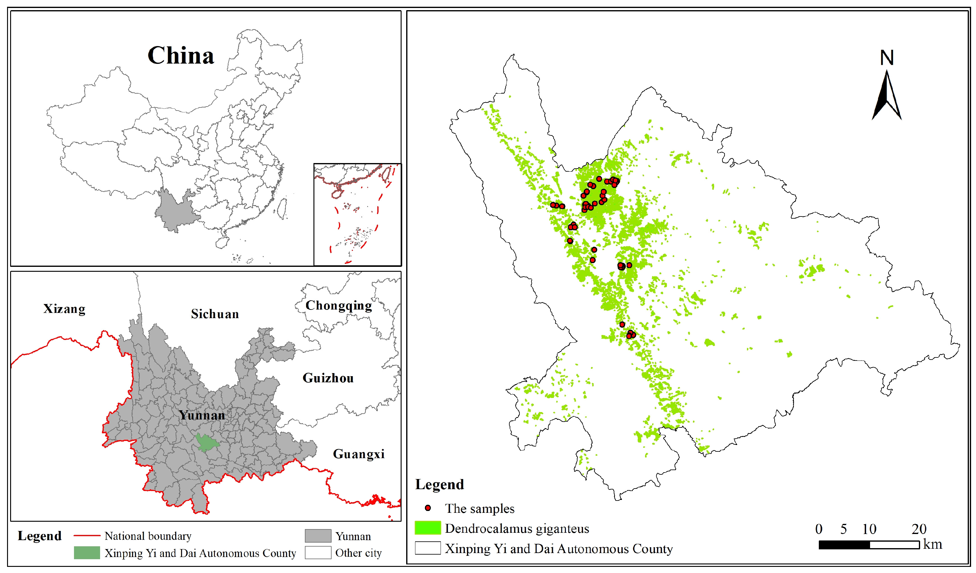
2.1. Study Area
2.2. Datasets and Preprocessing
2.2.1. Ground Survey Data Collection and Processing
2.2.2. ICESat-2/ATLAS Data
2.2.3. Sentinel-1/-2 Data
3. Research Methods and Data Processing
3.1. Research Methodology
3.1.1. Sequential Gaussian Conditional Simulation
- Feature variable normalization
- Variance function
- Principle of Sequential Gaussian Conditional Simulation
3.1.2. LAI Estimation Model
- Random Forest
- Gradient-Boosting Regression Trees
- K-Nearest Neighbors
3.1.3. Evaluation of Model Accuracy
3.2. Data Processing
3.2.1. Data Processing of ICESat-2/ATLAS
3.2.2. Data Processing of Sentinel-1/-2
3.2.3. Selection and Extraction of Feature Variables
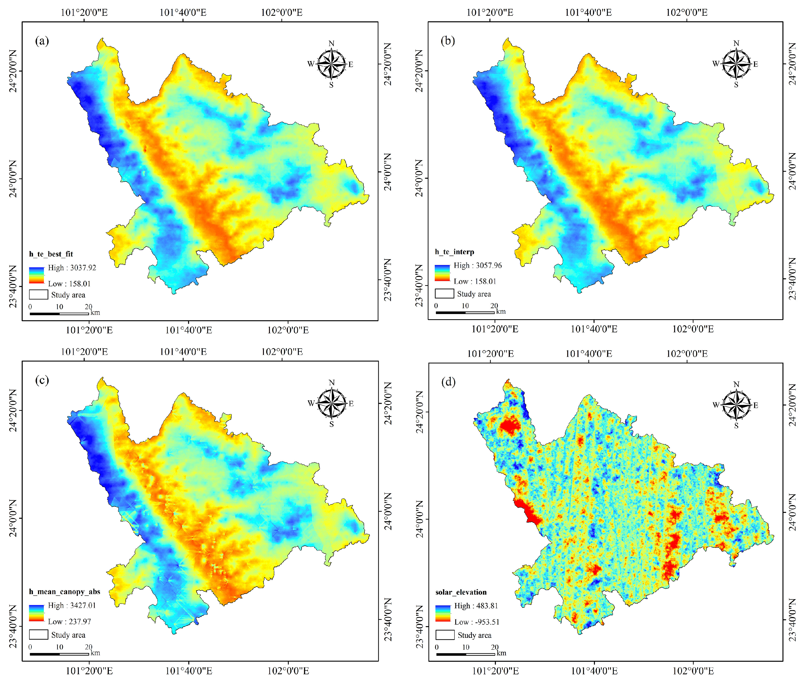
- ICESat-2/ATLAS parameters
- Extraction of region-scale remote sensing data and feature variables
4. Results and Analysis
4.1. Sequential Gaussian Condition Simulation Effect
4.1.1. Choice of Variance Function Model
4.1.2. Sequential Gaussian Condition Simulation of LAI Model Spot Feature Factors
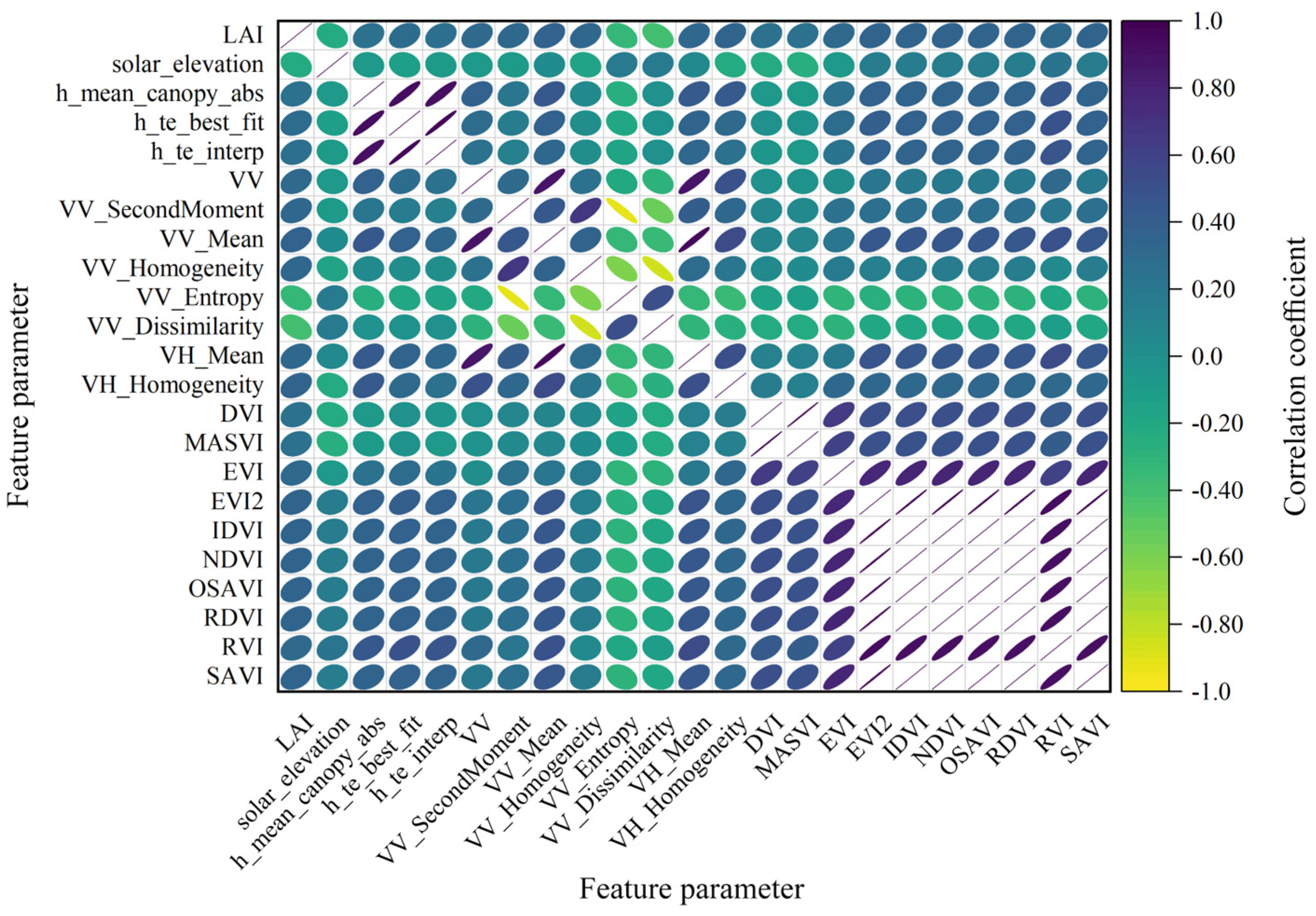
4.2. Variables Correlation Analysis
4.3. Estimation Results of Dendrocalamus giganteus LAI Model
4.4. Estimation Results of Combined Models of Different Remote Sensing Data Sources
4.4.1. Single ICESat-2/ATLAS Data
4.4.2. Combination of Different Remote Sensing Data Sources
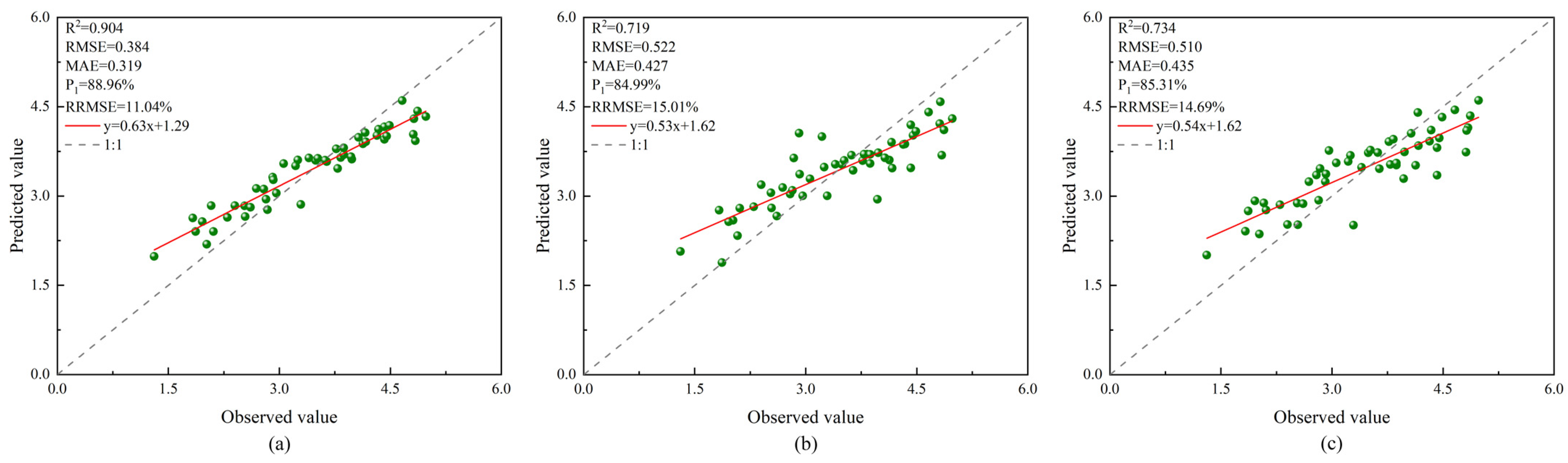
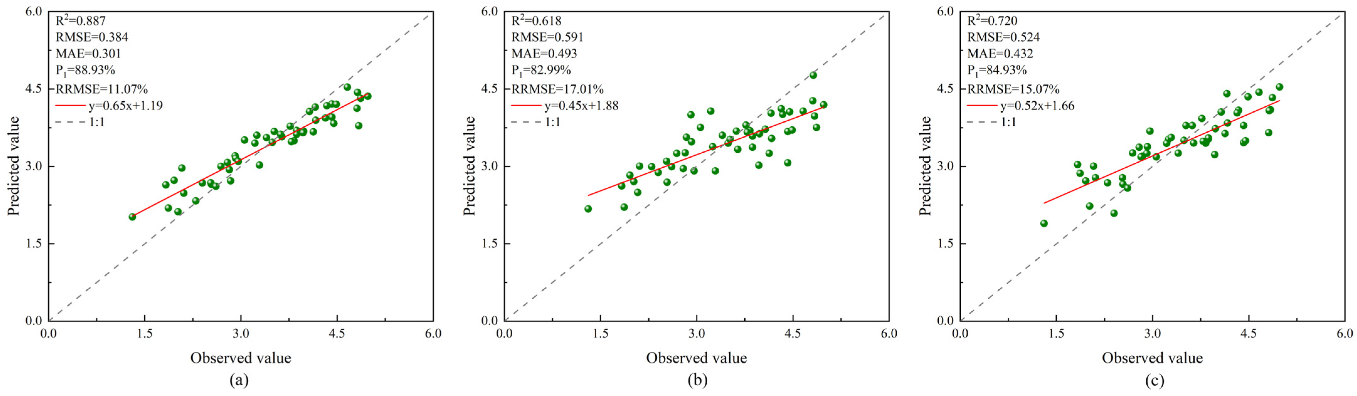
- Integration of ICESat-2/ATLAS and Sentinel-1 Data: The study opted for ICESat-2/ATLAS parameters, encompassing h_te_best_fit, h_te_interp, solar_elevation, and h_mean_canopy_abs, in conjunction with Sentinel-1 parameters VV_Mean and VV_Dissimilarity, as indicators for modeling purposes. The model’s effects are depicted in Figure 8a–c.
- Integration of ICESat-2/ATLAS and Sentinel-2 Data: The study selected parameters from ICE-Sat-2/ATLAS, encompassing h_te_best_fit, h_te_interp, solar_elevation, and h_mean_canopy_abs, in conjunction with Sentinel-2 parameters EVI2 and NDVI, to serve as modeling indicators. The performance of the model is depicted in Figure 9a–c.
4.4.3. Comparison of Model Effects
4.5. Spatial Distribution of LAI of Dendrocalamus giganteus in Xinping County
5. Discussion
5.1. Selection of Feature Factors
5.2. Difference in Estimation Accuracy of Different Data Sources
5.3. The Future Expandability of Geostatistical Methods
6. Conclusions
Author Contributions
Funding
Data Availability Statement
Acknowledgments
Conflicts of Interest
References
- Fang, H.; Baret, F.; Plummer, S.; Schaepman-Strub, G. An overview of global leaf area index (LAI): Methods, products, validation, and applications. Rev. Geophys. 2019, 57, 739–799. [Google Scholar] [CrossRef]
- Chen, J.M.; Black, T. Defining leaf area index for non-flat leaves. Plant Cell Environ. 1992, 15, 421–429. [Google Scholar] [CrossRef]
- Jonckheere, I.; Fleck, S.; Nackaerts, K.; Muys, B.; Coppin, P.; Weiss, M.; Baret, F. Review of methods for in situ leaf area index determination: Part I. Theories, sensors and hemispherical photography. Agric. For. Meteorol. 2004, 121, 19–35. [Google Scholar] [CrossRef]
- Wulder, M.A.; White, J.C.; Stinson, G.; Hilker, T.; Kurz, W.A.; Coops, N.C.; St-Onge, B.; Trofymow, J. Implications of differing input data sources and approaches upon forest carbon stock estimation. Environ. Monit. Assess. 2010, 166, 543–561. [Google Scholar] [CrossRef] [PubMed]
- Yan, G.; Hu, R.; Luo, J.; Weiss, M.; Jiang, H.; Mu, X.; Xie, D.; Zhang, W. Review of indirect optical measurements of leaf area index: Recent advances, challenges, and perspectives. Agric. For. Meteorol. 2019, 265, 390–411. [Google Scholar] [CrossRef]
- Fang, H. Retrieval of forest vertical leaf area index and clumping index through field measurement and remote sensing techniques: A review. Chin. Sci. Bull. 2021, 66, 3141–3153. [Google Scholar] [CrossRef]
- Lefsky, M.A.; Cohen, W.B.; Parker, G.G.; Harding, D.J. Lidar remote sensing for ecosystem studies: Lidar, an emerging remote sensing technology that directly measures the three-dimensional distribution of plant canopies, can accurately estimate vegetation structural attributes and should be of particular interest to forest, landscape, and global ecologists. BioScience 2002, 52, 19–30. [Google Scholar]
- Brunt, K.M.; Neumann, T.A.; Walsh, K.M.; Markus, T. Determination of local slope on the Greenland Ice Sheet using a multibeam photon-counting Lidar in preparation for the ICESat-2 Mission. IEEE Geosci. Remote Sens. Lett. 2013, 11, 935–939. [Google Scholar] [CrossRef]
- Zhu, X. Forest Height Retrieval of China with a Resolution of 30 m Using ICESat-2 and GEDI Data. Ph.D. Thesis, Aerospace Information Research Institute, Chinese Cademy of Sciences, Beijing, China, 2021. [Google Scholar]
- Narine, L.L.; Popescu, S.C.; Malambo, L. Using ICESat-2 to estimate and map forest aboveground biomass: A first example. Remote Sens. 2020, 12, 1824. [Google Scholar] [CrossRef]
- Yang, Z.; Shu, Q.; Qiu, S.; Xi, L. Regional-scale forest LAI estimation based on ICESat-2/ATLAS data combined with Kriging interpolation. J. Yunnan Univ. (Nat. Sci. Ed. ) 2023, 45, 1157–1170. [Google Scholar]
- Teng, J. Carbon Storage and Energy of Typical Sympodial Bamboo Ecosystems in China. Master’s Thesis, Zhejiang A and F University, Hangzhou, China, 2016. [Google Scholar]
- Ji, J.; Li, X.; Du, H.; Mao, F.; Fan, W.; Xu, Y.; Huang, Z.; Wang, J.; Kang, F. Multiscale leaf area index assimilation for Moso bamboo forest based on Sentinel-2 and MODIS data. Int. J. Appl. Earth Obs. Geoinf. 2021, 104, 102519. [Google Scholar] [CrossRef]
- Wang, C.; Huang, M.; Wnag, W.; Li, Z.; Zhang, T.; Ma, L.; Bai, Y.; Wang, Y.; Shi, J.; Long, R.; et al. Variation characteristics of plant community diversity and above-ground biomass in alpine degraded slopes along altitude gradients in the headwaters region of three-river on Tibetan plateau. Acta Ecol. Sin. 2022, 42, 3640–3655. [Google Scholar]
- Li, M.; Li, Y.; Zhao, W.; Wang, J. Characteristics and Geographical Distribution of Ancient Tree Groups in Xinping County. For. Inventory Plan. 2023, 48, 153–160. [Google Scholar]
- Zeng, Y.; Li, J.; Liu, Q.; Hu, R.; Mu, X.; Fan, W.; Xu, B.; Yin, G.; Wu, S. Extracting leaf area index by sunlit foliage component from downward-looking digital photography under clear-sky conditions. Remote Sens. 2015, 7, 13410–13435. [Google Scholar] [CrossRef]
- Markus, T.; Neumann, T.; Martino, A.; Abdalati, W.; Brunt, K.; Csatho, B.; Farrell, S.; Fricker, H.; Gardner, A.; Harding, D. The Ice, Cloud, and land Elevation Satellite-2 (ICESat-2): Science requirements, concept, and implementation. Remote Sens. Environ. 2017, 190, 260–273. [Google Scholar] [CrossRef]
- Xie, D.; Li, G.; Wang, J.; Guo, J.; Me, J.; Yang, C. An Overview of the Application Prospect of New Laser Altimetry Satellite ICESat-2 in Geoscience. Geomat. Spat. Inf. Technol. 2020, 43, 38–42+45. [Google Scholar]
- Torres, R.; Snoeij, P.; Geudtner, D.; Bibby, D.; Davidson, M.; Attema, E.; Potin, P.; Rommen, B.; Floury, N.; Brown, M. GMES Sentinel-1 mission. Remote Sens. Environ. 2012, 120, 9–24. [Google Scholar] [CrossRef]
- Drusch, M.; Del Bello, U.; Carlier, S.; Colin, O.; Fernandez, V.; Gascon, F.; Hoersch, B.; Isola, C.; Laberinti, P.; Martimort, P. Sentinel-2: ESA’s optical high-resolution mission for GMES operational services. Remote Sens. Environ. 2012, 120, 25–36. [Google Scholar] [CrossRef]
- Phiri, D.; Simwanda, M.; Salekin, S.; Nyirenda, V.R.; Murayama, Y.; Ranagalage, M. Sentinel-2 data for land cover/use mapping: A review. Remote Sens. 2020, 12, 2291. [Google Scholar] [CrossRef]
- WANG, M.; Fan, C.; GAO, B.; REN, Z.; LI, F. A spatial random forest interpolation method with semi-variogram. Chin. J. Eco-Agric. 2022, 30, 451–457. [Google Scholar]
- Hock, B.; Payn, T.; Shirley, J. Using a geographic information system and geostatistics to estimate site index of Pinus radiata for Kaingaroa Forest, New Zealand. New Zealand J. For. Sci. 1993, 23, 264–277. [Google Scholar]
- Berterretche, M.; Hudak, A.T.; Cohen, W.B.; Maiersperger, T.K.; Gower, S.T.; Dungan, J. Comparison of regression and geostatistical methods for mapping Leaf Area Index (LAI) with Landsat ETM+ data over a boreal forest. Remote Sens. Environ. 2005, 96, 49–61. [Google Scholar] [CrossRef]
- Emery, X.; Peláez, M. Assessing the accuracy of sequential Gaussian simulation and cosimulation. Comput. Geosci. 2011, 15, 673–689. [Google Scholar] [CrossRef]
- Zhao, Y.; Hua, Q.; Chen, J. Comparison of kriging interpolation with conditional sequential Gaussian simulation in principles and case analysis of their application in study on soil spatial variation. Acta Pedofil. Sin. 2011, 48, 856–862. [Google Scholar]
- Matheron, G. Les variables régionalisées et leur estimation: Une application de la théorie de fonctions aléatoires aux sciences de la nature. 1965. Available online: https://cir.nii.ac.jp/crid/1130282273252256768 (accessed on 15 January 2024).
- Zhang, S.; Shao, M.; Li, D. Prediction of soil moisture scarcity using sequential Gaussian simulation in an arid region of China. Geoderma 2017, 295, 119–128. [Google Scholar] [CrossRef]
- Qu, M.; Li, W.; Zhang, C. Spatial distribution and uncertainty assessment of potential ecological risks of heavy metals in soil using sequential Gaussian simulation. Hum. Ecol. Risk Assess. Int. J. 2014, 20, 764–778. [Google Scholar] [CrossRef]
- Huang, J.; Liu, W.; Zeng, G.; Li, F.; Huang, X.; Gu, Y.; Shi, L.; Shi, Y.; Wan, J. An exploration of spatial human health risk assessment of soil toxic metals under different land uses using sequential indicator simulation. Ecotoxicol. Environ. Saf. 2016, 129, 199–209. [Google Scholar] [CrossRef] [PubMed]
- Olea, R.A.; Pawlowsky, V. Compensating for estimation smoothing in kriging. Math. Geol. 1996, 28, 407–417. [Google Scholar] [CrossRef]
- Zhao, Y.; Sun, Z.; Chen, J. Analysis and Comparison in Arithmetic for Kriging Interpolation and Sequential Gaussian Conditional Simula-tion. J. Geo-Inf. Sci. 2010, 12, 767–776. [Google Scholar]
- Luo, S.; Xu, L.; Yu, J.; Zhou, W.; Yang, Z.; Wang, S.; Guo, C.; Gao, Y.; Xiao, J.; Shu, Q. Sampling Estimation and Optimization of Typical Forest Biomass Based on Sequential Gaussian Conditional Simulation. Forests 2023, 14, 1792. [Google Scholar] [CrossRef]
- Breiman, L. Random forests. Mach. Learn. 2001, 45, 5–32. [Google Scholar] [CrossRef]
- Zhang, W.; Tang, L.; Chen, F.; Yang, J. Prediction for TBM Penetration Rate Using Four Hyperparameter Optimization Methods and Random Forest Model. J. Basic Sci. Eng. 2021, 29, 1186–1200. [Google Scholar] [CrossRef]
- Friedman, J.H. Greedy function approximation: A gradient boosting machine. Ann. Stat. 2001, 1189–1232. [Google Scholar] [CrossRef]
- Friedman, J.H. Stochastic gradient boosting. Comput. Stat. Data Anal. 2002, 38, 367–378. [Google Scholar] [CrossRef]
- Scheuber, M. Potentials and limits of the k-nearest-neighbour method for regionalising sample-based data in forestry. Eur. J. For. Res. 2010, 129, 825–832. [Google Scholar] [CrossRef]
- Ver Hoef, J.M.; Temesgen, H. A comparison of the spatial linear model to nearest neighbor (k-NN) methods for forestry applications. PLoS ONE 2013, 8, e59129. [Google Scholar] [CrossRef] [PubMed]
- Gjertsen, A.K. Accuracy of forest mapping based on Landsat TM data and a kNN-based method. Remote Sens. Environ. 2007, 110, 420–430. [Google Scholar] [CrossRef]
- Moghimi, A.; Darestani, A.T.; Mostofi, N.; Fathi, M.; Amani, M. Improving forest above-ground biomass estimation using genetic-based feature selection from Sentinel-1 and Sentinel-2 data (case study of the Noor forest area in Iran). Kuwait J. Sci. 2024, 51, 100159. [Google Scholar] [CrossRef]
- Cai, W.; Zhao, S.; Wang, Y.; Peng, F. Estimation of winter wheat residue cover using spectral and textural information from Sentinel-2 data. Natl. Remote Sens. Bull. 2020, 24, 1108–1119. [Google Scholar] [CrossRef]
- Chen, B.; Pang, Y.; Li, Z.; North, P.; Rosette, J.; Sun, G.; Suárez, J.; Bye, I.; Lu, H. Potential of forest parameter estimation using metrics from photon counting LiDAR data in Howland Research Forest. Remote Sens. 2019, 11, 856. [Google Scholar] [CrossRef]
- Ghosh, S.M.; Behera, M.D.; Paramanik, S. Canopy height estimation using sentinel series images through machine learning models in a mangrove forest. Remote Sens. 2020, 12, 1519. [Google Scholar] [CrossRef]
- Jiang, F.; Sun, H.; Li, C.; Ma, K.; Chen, S.; Long, J.; Ren, L. Retrieving the forest aboveground biomass by combining the red edge bands of Sentinel-2 and GF-6. Acta Ecol. Sin 2021, 41, 8222–8236. [Google Scholar]
- Wu, G.; Fang, Y.; Jiang, Q.; Cui, M.; Li, N.; Ou, Y.; Diao, Z.; Zhang, B. Early identification of strawberry leaves disease utilizing hyperspectral imaging combing with spectral features, multiple vegetation indices and textural features. Comput. Electron. Agric. 2023, 204, 107553. [Google Scholar] [CrossRef]
- Rouse, J. Monitoring the Vernal Advancement and Retrogradation of Natural Vegetation. NASA/GSFCT Type II Report. 1973. Available online: https://cir.nii.ac.jp/crid/1570291224983494528 (accessed on 15 January 2024).
- Clevers, J. The application of a vegetation index in correcting the infrared reflectance for soil background. In Proceedings of the Symposium on Remote Sensing for Research and Development in Environmental Management, Enschede, The Netherlands, 21–24 April 1986; pp. 221–226. [Google Scholar]
- Huete, A.R. A soil-adjusted vegetation index (SAVI). Remote Sens. Environ. 1988, 25, 295–309. [Google Scholar] [CrossRef]
- Rondeaux, G.; Steven, M.; Baret, F. Optimization of soil-adjusted vegetation indices. Remote Sens. Environ. 1996, 55, 95–107. [Google Scholar] [CrossRef]
- Huete, A.; Didan, K.; Miura, T.; Rodriguez, E.P.; Gao, X.; Ferreira, L.G. Overview of the radiometric and biophysical performance of the MODIS vegetation indices. Remote Sens. Environ. 2002, 83, 195–213. [Google Scholar] [CrossRef]
- Jiang, Z.; Huete, A.R.; Didan, K.; Miura, T. Development of a two-band enhanced vegetation index without a blue band. Remote Sens. Environ. 2008, 112, 3833–3845. [Google Scholar] [CrossRef]
- Pearson, R.L.; Miller, L.D. Remote mapping of standing crop biomass for estimation of the productivity of the shortgrass prairie, Pawnee National Grasslands, Colorado. In Proceedings of the Eighth International Symposium on Remote Sensing of Environment, Ann Arbor, MI, USA, 2–6 October 1972. [Google Scholar]
- Qi, J.; Chehbouni, A.; Huete, A.R.; Kerr, Y.H.; Sorooshian, S. A modified soil adjusted vegetation index. Remote Sens. Environ. 1994, 48, 119–126. [Google Scholar] [CrossRef]
- Gitelson, A.A.; Merzlyak, M.N. Remote sensing of chlorophyll concentration in higher plant leaves. Adv. Space Res. 1998, 22, 689–692. [Google Scholar] [CrossRef]
- Rouse, J.W.; Haas, R.H.; Schell, J.A.; Deering, D.W. Monitoring vegetation systems in the Great Plains with ERTS. NASA Spec. Publ 1974, 351, 309. [Google Scholar]
- Rouse Jr, J.W.; Haas, R.H.; Deering, D.; Schell, J.; Harlan, J.C. Monitoring the Vernal Advancement and Retrogradation (Green Wave Effect) of Natural Vegetation. 1974. Available online: https://ntrs.nasa.gov/citations/19750020419 (accessed on 15 January 2024).
- Xu, C.; Pu, L.; Zhu, M.; XU, C.; Zhang, M.; Xu, Y. Prediction of Soil Heavy Metals Content Based on Sequential Gaussian Simulation and Evaluation of Its Uncertainties: A Case Study of Soil Hg Content in Yixing. Acta Pedol. Sin. 2018, 55, 999–1006. [Google Scholar]
- Zhang, W.; Zhao, L.; Li, Y.; Shi, J.; Yan, M.; Ji, Y. Forest Above-Ground Biomass Inversion Using Optical and SAR Images Based on a Multi-Step Feature Optimized Inversion Model. Remote Sens. 2022, 14, 1608. [Google Scholar] [CrossRef]
- Zhao, P.; Lu, D.; Wang, G.; Wu, C.; Huang, Y.; Yu, S. Examining spectral reflectance saturation in Landsat imagery and corresponding solutions to improve forest aboveground biomass estimation. Remote Sens. 2016, 8, 469. [Google Scholar] [CrossRef]
- Shu, Q.; Xi, L.; Wang, K.; Xie, F.; Pang, Y.; Song, H. Optimization of samples for remote sensing estimation of forest aboveground biomass at the regional scale. Remote Sens. 2022, 14, 4187. [Google Scholar] [CrossRef]
- Feng, X.; Tan, S.; Dong, Y.; Zhang, X.; Xu, J.; Zhong, L.; Yu, L. Mapping large-scale bamboo forest based on phenology and morphology features. Remote Sens. 2023, 15, 515. [Google Scholar] [CrossRef]
- Luo, T.; Neilson, R.P.; Tian, H.; Vörösmarty, C.J.; Zhu, H.; Liu, S. A model for seasonality and distribution of leaf area index of forests and its application to China. J. Veg. Sci. 2002, 13, 817–830. [Google Scholar] [CrossRef]
- Wu, J.; Chen, P.; Fu, S.; Chen, Q.; Pan, X. Co-inversion of island leaf area index combination morphological and spectral parameters based on UAV multi-source remote sensing data. Ecol. Inform. 2023, 77, 102190. [Google Scholar] [CrossRef]
- Mutanga, O.; Masenyama, A.; Sibanda, M.J.I.J.o.P.; Sensing, R. Spectral saturation in the remote sensing of high-density vegetation traits: A systematic review of progress, challenges, and prospects. ISPRS J. Photogramm. Remote Sens. 2023, 198, 297–309. [Google Scholar] [CrossRef]
- Davi, H.; Soudani, K.; Deckx, T.; Dufrene, E.; Le Dantec, V.; Francois, C. Estimation of forest leaf area index from SPOT imagery using NDVI distribution over forest stands. Int. J. Remote Sens. 2006, 27, 885–902. [Google Scholar] [CrossRef]
- Zhou, W.; Shu, Q.; Wang, S.; Yang, Z.; Luo, S.; Xu, L.; Xiao, J. Estimation of forest canopy closure in northwest Yunnan based on multi-source remote sensing data colla-boration. Chin. J. Appl. Ecol. 2023, 34, 1806–1816. [Google Scholar] [CrossRef]
- Yang, X.; Wang, C.; Pan, F.; Nie, S.; Xi, X.; Luo, S. Retrieving leaf area index in discontinuous forest using ICESat/GLAS full-waveform data based on gap fraction model. ISPRS J. Photogramm. Remote Sens. 2019, 148, 54–62. [Google Scholar] [CrossRef]
- Korhonen, L.; Packalen, P.; Rautiainen, M. Comparison of Sentinel-2 and Landsat 8 in the estimation of boreal forest canopy cover and leaf area index. Remote Sens. Environ. 2017, 195, 259–274. [Google Scholar] [CrossRef]
- Stankevich, S.A.; Kozlova, A.A.; Piestova, I.O.; Lubskyi, M.S. Leaf area index estimation of forest using sentinel-1 C-band SAR data. In Proceedings of the 2017 IEEE Microwaves, Radar and Remote Sensing Symposium (MRRS), Kiev, Ukraine, 29–31 August 2017; pp. 253–256. [Google Scholar]
- Rosso, P.; Nendel, C.; Gilardi, N.; Udroiu, C.; Chlebowski, F. Processing of remote sensing information to retrieve leaf area index in barley: A comparison of methods. Precis. Agric. 2022, 23, 1449–1472. [Google Scholar] [CrossRef]
- Wang, J.; Xiao, X.; Bajgain, R.; Starks, P.; Steiner, J.; Doughty, R.B.; Chang, Q. Estimating leaf area index and aboveground biomass of grazing pastures using Sentinel-1, Sentinel-2 and Landsat images. ISPRS J. Photogramm. Remote Sens. 2019, 154, 189–201. [Google Scholar] [CrossRef]


| Sample Size | Minimum Value | Maximum Value | Mean Value | Standard Deviation | Variance |
|---|---|---|---|---|---|
| 51 | 1.31 | 4.98 | 3.43 | 0.94 | 0.89 |
| Variable Factor Name | Meaning | Describe |
|---|---|---|
| solar_elevation | Solar elevation | Solar angle above or below the plane tangent to the ellipsoid surface at the laser spot. |
| h_mean_canopy_abs | Absolute mean canopy height | Mean of the individual absolute canopy heights within the segment referenced above the WGS84 Ellipsoid. |
| h_te_best_fit | Segment terrain height best fit | The best-fit terrain elevation at the mid-point location of each 100 m segment. |
| h_te_interp | Interpolated | Interpolated terrain surface height above the WGS84. |
| Texture Feature Parameter | Equation | Texture Feature Parameter | Equation |
|---|---|---|---|
| Mean (ME) | Dissimilarity (DI) | ||
| Variance (VA) | Entropy (EN) | ||
| Homogeneity (HO) | Second Moment (SM) | ||
| Contrast (CO) | Correlation (CR) |
| Vegetation Index Name | Calculation Formula |
|---|---|
| Normalized Difference Vegetation Index (NDVI) [47] | |
| Difference Vegetation Index (DVI) [48] | |
| Soil-Adjusted Vegetation Index (SAVI) [49] | |
| Optimized Soil-Adjusted Vegetation Index (OSAVI) [50] | |
| Enhanced Vegetation Index (EVI) [51] | |
| Two-band Enhanced Vegetation Index (EVI2) [52] | |
| Ratio Vegetation Index (RVI) [53] | |
| Modified Soil-Adjusted Vegetation Index (MSAVI) [54] | |
| Green Normalized Difference Vegetation Index (GNDVI) [55] | |
| Green Ratio Vegetation Index (GRVI) [56] | |
| Renormalized Difference Vegetation Index (RDVI) [56] | |
| Infrared Difference Vegetation Index (IDVI) [57] |
| Data Source | Variable Type | Variable Name | Variables Number |
|---|---|---|---|
| Sentinel-1 | Backscatter coefficient | VV, VH | 2 |
| Texture features | VV-ME, VV-VA, VV-HO, VV-CO, VV-DI, VV-EN, VV-SM, VV-CR, VH-ME, VH-VA, VH-HO, VH-CO, VH-DI, VH-EN, VH-SM, VH-CR, | 16 | |
| Sentinel-2 | Original single spectral bands | B2, B3, B4, B5, B6, B7, B8, B8A | 8 |
| Vegetation Index | NDVI, DVI, SAVI, OSAVI, EVI, EVI2, RVI, MSAVI, GNDVI, GRVI, RDVI, IDVI | 12 |
| Modeling Factors | Model | R2 | RSS | C0 | C0 + C | C0/C0 + C/% | Range/m |
|---|---|---|---|---|---|---|---|
| h_te_best_fit | Linear | 0.482 | 3.720 | 1.115120 | 2.736242 | 0.592 | 52,262.12 |
| Spherical | 0.921 | 0.567 | 0.051000 | 2.397000 | 0.979 | 27,500.00 | |
| Exponential | 0.870 | 1.000 | 0.001000 | 2.465000 | 1.000 | 33,300.00 | |
| Gaussian | 0.914 | 0.618 | 0.314000 | 2.392000 | 0.869 | 22,516.66 | |
| h_te_interp | Linear | 0.482 | 3.720 | 1.115268 | 2.736374 | 0.592 | 52,262.12 |
| Spherical | 0.921 | 0.567 | 0.052000 | 2.398000 | 0.978 | 27,600.00 | |
| Exponential | 0.870 | 1.000 | 0.001000 | 2.465000 | 1.000 | 33,300.00 | |
| Gaussian | 0.914 | 0.618 | 0.319000 | 2.392000 | 0.867 | 22,516.66 | |
| h_mean_canopy_abs | Linear | 0.492 | 2.740 | 1.074694 | 2.495106 | 0.569 | 52,262.12 |
| Spherical | 0.925 | 0.406 | 0.163000 | 2.197000 | 0.926 | 27,800.00 | |
| Exponential | 0.877 | 0.687 | 0.001000 | 2.249000 | 1.000 | 31,800.00 | |
| Gaussian | 0.917 | 0.447 | 0.394000 | 2.192000 | 0.820 | 22,689.87 | |
| solar_elevation | Linear | 0.254 | 1.214000 | 1741.631 | 2302.117 | 0.243 | 52,262.12 |
| Spherical | 0.740 | 4.24100 | 710.0000 | 2151.000 | 0.670 | 13,000.00 | |
| Exponential | 0.690 | 5.04300 | 259.0000 | 2152.000 | 0.880 | 11,700.00 | |
| Gaussian | 0.732 | 4.35900 | 947.0000 | 2151.000 | 0.560 | 11,085.13 |
| Data Source | Parameters and Correlations |
|---|---|
| ICESat-2/ATLAS | h_te_best_fit (0.298) **, h_te_interp (0.271) *, solar_elevation (−0.236) *, h_mean_canopy_abs (0.248) * |
| Sentinel-1 | VV_Mean (0.367) ***, VV_Dissimilarity (−0.384) ***, VV (0.315) **, VV_SecondMoment (0.336) **, VV_Homogeneity (0.324) **, VV_Entropy (−0.336) **, VH_Mean (0.329) **, VH_Homogeneity (0.352) ** |
| Sentinel-2 | EVI (0.319) **, EVI2 (0.343) **, NDVI (0.341) **, IDVI (0.341) **, OSAVI (0.341) **, RDVI (0.341) **, RVI (0.31) **, SAVI (0.341) **, DVI (0.252) *, MSAVI (0.243) * |
| Parameter Category | Model Parameters | RF Model Accuracy | GBRT Model Accuracy | KNN Model Accuracy |
|---|---|---|---|---|
| ICESat-2/ATLAS, Sentinel-1, Sentinel-2 | h_te_best_fit, h_te_interp, h_mean_canopy_abs, solar_elevation, VV_Mean, VV_Dissimilarity, EVI2, NDVI | R2 = 0.904 RMSE = 0.384 MAE = 0.319 P1 = 88.96% RRMSE = 11.04% | R2 = 0.719 RMSE = 0.522 MAE = 0.427 P1 = 84.99% RRMSE = 15.01% | R2 = 0.734 RMSE = 0.510 MAE = 0.435 P1 = 85.31% RRMSE = 14.69% |
| ICESat-2/ATLAS | h_te_best_fit, h_te_interp, h_mean_canopy_abs, solar_elevation | R2 = 0.862 RMSE = 0.422 MAE = 0.364 P1 = 87.84% RRMSE = 12.16% | R2 = 0.565 RMSE = 0.612 MAE = 0.513 P1 = 82.39% RRMSE = 17.61% | R2 = 0.650 RMSE = 0.577 MAE = 0.476 P1 = 83.40% RRMSE = 16.60% |
| ICESat-2/ATLAS, Sentinel-1 | h_te_best_fit, h_te_interp, solar_elevation, h_mean_canopy_abs, VV_Mean, VV_Dissimilarity | R2 = 0.887 RMSE = 0.384 MAE = 0.301 P1 = 88.93% RRMSE = 11.07% | R2 = 0.618 RMSE = 0.591 MAE = 0.493 P1 = 82.99% RRMSE = 17.01% | R2 = 0.720 RMSE = 0.524 MAE = 0.432 P1 = 84.93% RRMSE = 15.07% |
| ICESat-2/ATLAS, Sentinel-2 | h_te_best_fit, h_te_interp, h_mean_canopy_abs, solar_elevation, EVI2, NDVI | R2 = 0.896 RMSE = 0.402 MAE = 0.345 P1 = 88.42% RRMSE = 11.58% | R2 = 0.669 RMSE = 0.542 MAE = 0.434 P1 = 84.41% RRMSE = 15.59% | R2 = 0.673 RMSE = 0.556 MAE = 0.461 P1 = 84.00% RRMSE = 16.00% |
Disclaimer/Publisher’s Note: The statements, opinions and data contained in all publications are solely those of the individual author(s) and contributor(s) and not of MDPI and/or the editor(s). MDPI and/or the editor(s) disclaim responsibility for any injury to people or property resulting from any ideas, methods, instructions or products referred to in the content. |
© 2024 by the authors. Licensee MDPI, Basel, Switzerland. This article is an open access article distributed under the terms and conditions of the Creative Commons Attribution (CC BY) license (https://creativecommons.org/licenses/by/4.0/).
Share and Cite
Qin, Z.; Yang, H.; Shu, Q.; Yu, J.; Xu, L.; Wang, M.; Xia, C.; Duan, D. Estimation of Leaf Area Index for Dendrocalamus giganteus Based on Multi-Source Remote Sensing Data. Forests 2024, 15, 1257. https://doi.org/10.3390/f15071257
Qin Z, Yang H, Shu Q, Yu J, Xu L, Wang M, Xia C, Duan D. Estimation of Leaf Area Index for Dendrocalamus giganteus Based on Multi-Source Remote Sensing Data. Forests. 2024; 15(7):1257. https://doi.org/10.3390/f15071257
Chicago/Turabian StyleQin, Zhen, Huanfen Yang, Qingtai Shu, Jinge Yu, Li Xu, Mingxing Wang, Cuifen Xia, and Dandan Duan. 2024. "Estimation of Leaf Area Index for Dendrocalamus giganteus Based on Multi-Source Remote Sensing Data" Forests 15, no. 7: 1257. https://doi.org/10.3390/f15071257
APA StyleQin, Z., Yang, H., Shu, Q., Yu, J., Xu, L., Wang, M., Xia, C., & Duan, D. (2024). Estimation of Leaf Area Index for Dendrocalamus giganteus Based on Multi-Source Remote Sensing Data. Forests, 15(7), 1257. https://doi.org/10.3390/f15071257