Article

Spatial Pattern and Environmental Driving Factors of Treeline Elevations in Yulong Snow Mountain, China

School of Soil and Water Conservation, Southwest Forestry University, Kunming 650224, China
*
Author to whom correspondence should be addressed.
Forests 2024, 15(7), 1261; https://doi.org/10.3390/f15071261
Submission received: 11 June 2024 / Revised: 16 July 2024 / Accepted: 17 July 2024 / Published: 19 July 2024
(This article belongs to the Section Forest Ecology and Management)

Abstract

:
The southwestern region of China is a global biodiversity hotspot. Understanding the environmental mechanisms behind treeline formation in high-altitude areas is crucial for predicting ecosystem changes, such as the upward movement of the treeline due to climate warming and the disappearance of high-altitude rocky beach and shrub ecosystems. Globally, observations show that growing seasonal temperatures at treelines are typically 6–7 °C, but trees do not always reach the predicted elevations. Spatial heterogeneity exists in the deviation (Dtreeline) between actual treeline elevation and the thermal treeline; however, the main driving factors for Dtreeline in many areas remain unclear. This study uses Yulong Snow Mountain as an example, employing machine learning methods like Support Vector Machine (SVM) to precisely identify actual treeline elevation and Extreme Gradient Boosting Tree (XGBoost) to explore the main environmental factors driving the spatial heterogeneity of Dtreeline. Our research found that (1) more than half of the treelines deviated from the thermal treeline, with the average elevation of the thermal treeline (3924 ± 391 m) being about 56 m higher than the actual treeline (3863 ± 223 m); (2) Dtreeline has a complex relationship with environmental factors. In addition to being highly correlated with temperature, precipitation and wind speed also significantly influence the treeline in this region; and (3) the influence of individual variables such as precipitation and wind speed on the spatial variation of Dtreeline is limited, often nonlinear, and involves threshold effects. This knowledge is essential for developing comprehensive protection strategies for Yunnan’s high-altitude ecological systems in response to climate warming. Furthermore, it plays a significant role in understanding the changes in biological communities and the response of high-altitude areas to climate change.

1. Introduction

At high elevation or latitude, trees reach the altitude limit of the low-temperature boundary, forming a potential upper range limit known as the treeline [1,2,3]. This is also defined as the general cold edge of the basic ecological niche of trees and is one of the most important bioclimatic reference lines in nature [3,4]. It is believed that treelines on the global scale have a unified formation mechanism, following the same climatic envelope [5,6]. Extensive observational experiments have calculated the seasonal average temperature of treelines to be 6.4 ± 0.8 °C and the shortest seasonal length to be 94 days [5,7], referred to hereafter as the thermal treeline. In the real world, trees do not always reach the position of realizing their fundamental niches locally or regionally; the upper limit that trees can reach may be restricted to a lower altitude [2,8]. While the temperature during the growing season is not influenced by altitude, latitude (seasonal length), bedrock type, soil fertility, humidity (above minimum levels), and thermal extremes, all of these factors can affect tree growth [3,9,10]. By studying the degree of deviation (Dtreeline) between the actual treeline and the thermal treeline, we can better understand the key driving factors and processes that determine vegetation cover [11,12]. This understanding is crucial for accurately estimating the potential expansion of tree cover near the treeline in warmer climates, which has significant implications for plant community recombination and biodiversity.
It is believed that treelines rise with climate warming [13,14]. However, globally, treeline positions exhibit varying trends in response to climate warming, such as rising, remaining unchanged, or even falling [15,16,17,18,19]. One reason for the inconsistency between rising average temperatures and the expected treeline response may be the spatial non-uniformity of temperature changes. Over the past century, there have been significant differences in average temperature changes at local or regional levels across different areas [20,21,22]. Additionally, temperature may not be the dominant factor controlling treeline positions, as its direct impact can be masked by the interaction of other factors, such as precipitation [23,24], disturbances [25,26,27], light suppression [28,29], or plant-to-plant interactions [30,31]. Furthermore, significant differences in terrain and local climate among various treelines mean that overlooking local variations may lead to an overemphasis on temperature as a driving factor at broader scales [15,32].
Due to the unique geographical location and harsh conditions of mountainous regions, obtaining accurate field data is challenging [33,34,35]. Using satellite data, particularly the Normalized Difference Vegetation Index (NDVI), has long been a primary method for monitoring forest dynamics [36,37]. However, the forest boundaries extracted based on these indices have low resolution, and the reflectance from bare rocks, sparse vegetation, and scattered trees in the treeline can cause significant variability in NDVI values [37,38,39]. In recent years, machine learning methods have been successfully applied in forest dynamics monitoring [40] and alpine treeline ecological modeling and prediction [4]. For instance, Wang et al. [41]. demonstrated that convolutional neural networks could monitor vegetation changes in alpine treeline ecotones, allowing for the assessment of large-scale long-term vegetation dynamics at fine spatial resolutions. Nguyen et al. [42]. developed an interpretable deep learning model for forest mapping, finding that rule-based models can quantify intermediate key variables and predict forest maps reflecting forest definitions. Additionally, the development of LiDAR has made it easier to obtain tree structure data in treeline areas [43]. Combining LiDAR with machine learning methods allows researchers to more accurately identify treeline elevation, forest health conditions, and vegetation change trends, providing more reliable ecological management decision support, a trend that is continually strengthening [40,44].
Yulong Snow Mountain is the southernmost extent of modern glaciation in Asia and is significantly affected by global warming [45,46]. The treeline, as a transitional zone from forest to alpine or tundra habitats, is a tension zone where one vegetation type replaces another, making it a vulnerable part of the ecosystem. Numerous observations have found that some cold-tolerant plants that previously thrived in colder areas have died due to rising temperatures, and some plants have been affected by pest infestations. However, due to the lack of technical capabilities, changes in the treeline of Yulong Snow Mountain have not been monitored over previous decades, making it impossible to accurately measure treeline fluctuations. Research on the treeline of Yulong Snow Mountain at a fine scale has become an urgent issue to address. This study utilizes LiDAR tree height data to identify the actual treeline distribution with support vector machines (SVMs). By employing XGBoost (Extreme Gradient Boosting), it investigates environmental factors contributing to variations between the actual treeline and the thermal treeline. This research provides scientific evidence for developing more effective conservation strategies to address future ecological changes and challenges.

2. Materials and Methods
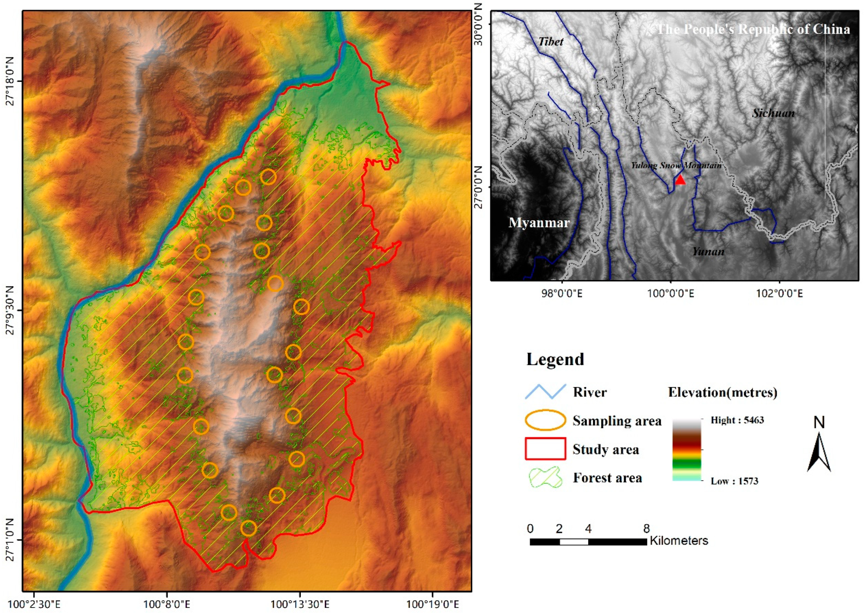
2.1. Study Area

Yulong Snow Mountain (100°4′2″–100°16′30″ N, 27°3′2″–27°18′57″ E) is the northern hemisphere’s closest mountain range to the equator with year-round snow cover. Located at the southeast end of the Hengduan Mountains (see Figure 1), its highest peak reaches an altitude of 5596 m [47]. The 13 peaks of the range are aligned vertically from south to north, and the area is rich in natural and cultural resources. In 1984, the Yulong Snow Mountain Provincial Nature Reserve was established in Yunnan, China. Situated within the southern temperate plateau monsoon climate zone, Yulong Snow Mountain experiences unique mountain monsoon characteristics and is influenced by westerly circulation, southwest monsoon, and southeast monsoon. The region has distinct dry and wet seasons: the dry season spans from November to April with minimal rainfall, while the wet season from May to October accounts for over 90% of the annual rainfall. The average annual temperature is 12.79 °C, and the area receives an average of 2530 h of sunshine annually. From the valley to the mountaintop, the average temperature decreases by about 0.86 °C for every 100 m of elevation gain.
Yulong Snow Mountain is a significant biodiversity hotspot in northwest Yunnan, serving as a crucial transitional area that connects the vegetation distributions of northwest and central Yunnan. It is the most concentrated area of high-altitude plant flora in the Hengduan Mountains of northwest Yunnan [48]. The mountain’s subalpine coniferous forest belt, at altitudes of 3100–3800 m, comprises fir, redwood, and spruce forests (both pure and mixed). Between 3800 and 4500 m, there is a high mountain shrub meadow zone, with alpine shrub meadows below 4100 m mainly consisting of various cushion or creeping azaleas. From 4100 to 4350 m, only scattered high mountain rocky beach plants are found [49]. Yulong Snow Mountain hosts 96 rare and endangered protected species from 20 families and 50 genera. The area also has 59 recorded wild economic animal species, including 57 mammal species from 8 orders, 21 families, and 42 genera [48,50]. These species are mostly found in high-altitude, sparsely populated areas and are characterized by high diversity but low population numbers. On 7 August 2019, researchers from the Lijiang Alpine Botanical Garden, Kunming Institute of Botany, Chinese Academy of Sciences, discovered a wild population of the endangered plant Cypripedium yulongensis (Cypripedium forrestii Cribb), which is endemic to China, during their field survey in Yulong Snow Mountain.

2.2. Data and Methods

Due to the complex terrain of the Yulong Snow Mountain region, with its intricate network of deep gullies, it is extremely challenging to identify the treeline solely through visual interpretation. Therefore, we aimed to use a model to assist in accurately mapping the actual treeline of Yulong Snow Mountain, ensuring that the identified treeline is both precise and continuous. Temperature is definitively the primary factor affecting the treeline. Besides temperature, we also wanted to determine whether other environmental variables significantly influence treeline elevation and whether their relationship with the treeline is linear or nonlinear.

2.2.1. Sampling and Feature Selection

To acquire the training samples required for the treeline recognition model, we manually delineated the treeline within the sampling areas using high-resolution (<5 m) satellite imagery from the Google Earth platform [2,51,52]. We established sampling areas along the boundary between the summit of Yulong Snow Mountain and the vegetation line at intervals of 3000 m. Each sampling area was circular with a radius of 500 m [4], and a total of 20 sampling areas were set up (as shown in Figure 1). To ensure a uniform quality of interpretation, we cross-validated the obtained samples using different interpreters and then had a single quality controller check all of the results. After digitizing all distinguishable treelines, the linear data were imported into ArcGIS 10.8 and converted to point data (generating a point every 20 m), resulting in a total of 3680 data points for subsequent model generation.
For the treeline recognition model, we primarily considered features related to elevation. We aimed to position the identified treeline as close to the upper boundary as possible, making the horizontal and vertical heights of the sample points relative to the summit essential. Given the complexity of the terrain, we incorporated a patented [53] technology that adds the feature of ‘surface roughness (ULS)’, which better represents the actual height of mountain ridges or the actual depth of valleys. We aimed for the model to identify treelines with minimal human interference. Thus, we included the feature of human activity footprint. We used a global record of annual terrestrial Human Footprint dataset from 2000 to 2018 [54], downloaded from https://github.com/HaoweiGis/humanFootprintMapping/, accessed on 17 January 2024. By averaging over multiple years, we obtained a map with a spatial resolution of 1 km showing the degree of human disturbance. This map integrates eight pressure variables that reflect human activity intensity, including built environments, population density, nighttime light, croplands, pasture lands, roadways, railways, and navigable waterways. Detailed information on the features can be found in Table 1 below:

2.2.2. LiDAR-Based Tree Height Data Processing and Verification

Trees forming the treeline should be life-form trees with a single, upright stem that reaches a height of at least 2–3 m [3,38,55]. Therefore, we needed to add a height restriction to the process of extracting the treeline. We used a 30 m resolution tree canopy height map [56] derived from GEDI point footprint data integrated with Landsat time-series data (Landsat ARD). This map was developed by the Global Land Analysis and Discovery laboratory at the University of Maryland and downloaded from https://glad.umd.edu/dataset/gedi/, accessed on 10 July 2023. First, we segmented the tree canopy height map into forest and non-forest areas, assigning a value of 1 to forest areas where the tree height exceeded 3 m and 0 to other areas. To eliminate the interference of inner non-forest patches and outer small forest patches, we used the majority filter tool in ArcGIS 10.8 to fill small internal holes and remove small external patches. The processed binary map was then converted into polygon vectors, from which edge lines were extracted and further converted into points (one point every 20 m along the lines). The recognition model identifies the actual treeline points from these points.

2.2.3. SVM Model and the Actual Treeline Data

SVM (support vector machine) is a binary classification model aimed at finding the most suitable “margin” to divide a dataset [57]. It is well-suited for small to medium-sized datasets, nonlinear, and high-dimensional classification problems. The current version (soft margin) was introduced by Corinna Cortes and Vapnik in 1993 [58], making SVM more flexible and robust in handling linearly inseparable data [59,60]. The data extracted in the previous step can be roughly divided into two categories (upper boundary points and lower boundary points). Therefore, we believe that the SVM algorithm is suitable for constructing the recognition model as it can find an appropriate “margin” to distinguish between treeline and non-treeline points.
We hope that the SVM model can use more test samples to ensure its accuracy. Seventy percent (n = 2578) of the data were randomly assigned to the training dataset, while thirty percent (n = 1104) were used as the test dataset. To measure the accuracy of the model, we used a confusion matrix, a table with two rows and two columns that reports the number of true positives (TP), false negatives (FN), false positives (FP), and true negatives (TN). To make a comprehensive evaluation of the SVM model, precision (P) and recall (R) are two important evaluation indicators:
P = T P T P + F P
R = T P T P + F N
P and R have a trade-off relationship, meaning that in certain situations, improving one metric might lead to a decrease in the other. We aimed to improve the accuracy of identifying actual treelines as much as possible. Therefore, we only used elevations with a probability of 85% or higher in the model’s predicted results, ensuring precision above 85%. This operation was implemented using the ‘decision_function(X)’ function in the scikit-learn library in Python 3.10.13.

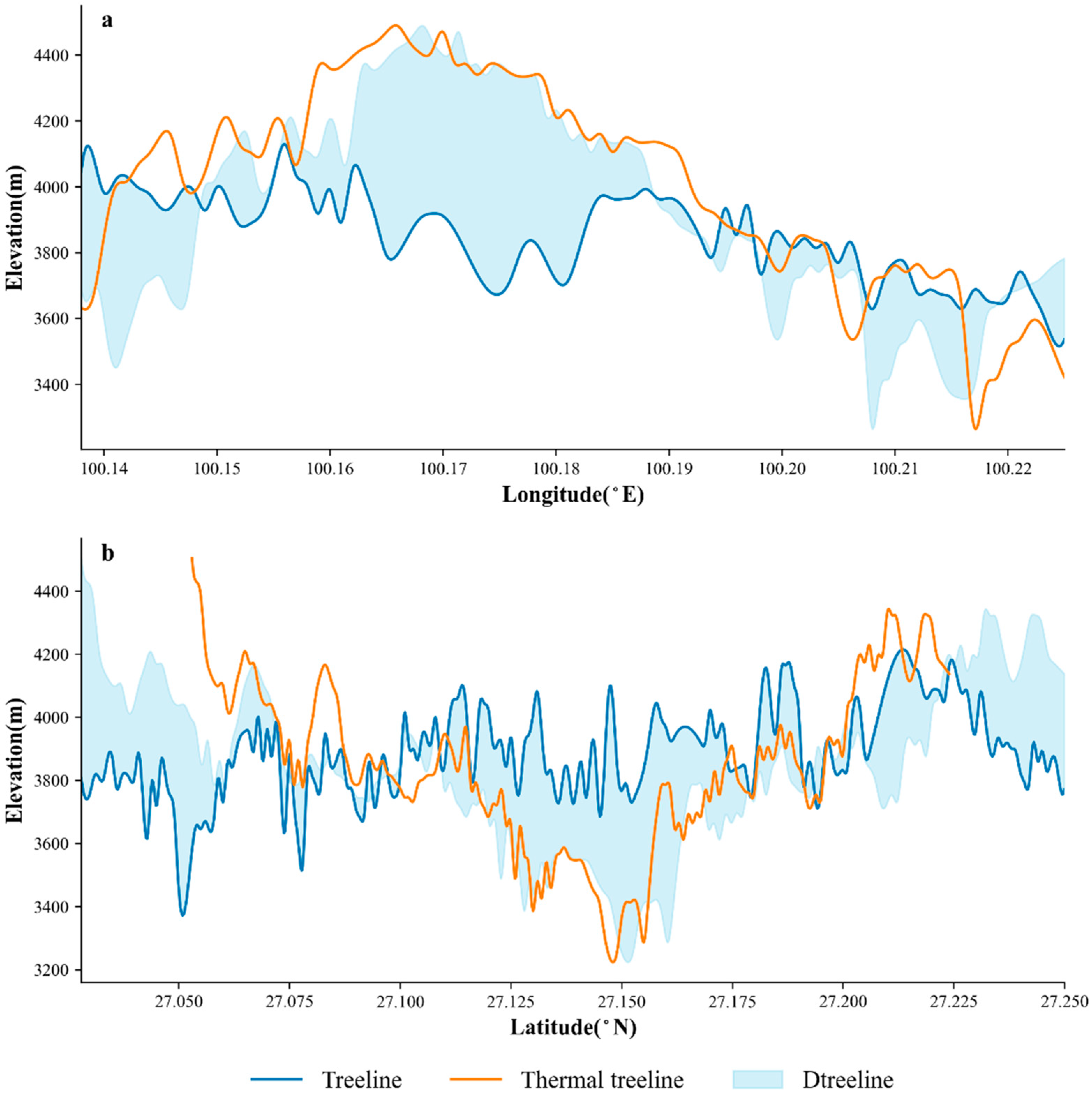
2.2.4. Thermal Treeline and Dtreeline

Referring to Paulsen and Körner’s (2014) global treeline observation experiment, we calculated the growing season temperature using 0.9 °C as the baseline [4,5,7]. Daily mean temperature was obtained from a long-term series of daily land surface temperature (TRIMS LST; 2000–2022) [61] by the National Tibetan Plateau Data Center (http://data.tp-dc.ac.cn, accessed on 10 March 2024). First, we calculated the number of days and the total temperature sum for each year from 2000 to 2019, where the daily mean temperature exceeded 0.9 °C. The total temperature sum was divided by the number of days to obtain the annual growing season average temperature. The final growing season temperature was obtained by averaging the 20-year growing season temperatures. In the calculated growing season temperature map, we marked the temperature range of 6.3–6.5 °C, which represents the thermal treeline value in this study.
KD Tree (k-Dimensional Tree) is a data structure used for efficient point queries and range searches in multi-dimensional space [62,63]. Using the KD Tree model, we queried the point on the actual treeline closest in latitude and longitude to the thermal treeline. Pairing the two elevation values and calculating the difference between them gives the Dtreeline value. The absolute value of the Dtreeline represents the deviation of the actual treeline from the theoretical treeline at 6.4 ± 0.8 °C. We used Dtreeline as the response variable in our statistical analysis. This response variable provides a standardized measure of treeline variation, eliminating confounding effects caused by the negative correlation between treeline altitude and latitude.

2.2.5. Environment Variable and XGBoost Model

The selection of environmental variables focuses on four aspects: climatic influences, soil substrate, disturbance activities, and topography, as detailed in Table 2. According to the Biometeorological Index published by the ECMWF (European Centre for Medium-Range Weather Forecasts), the climatic variables include daily mean temperature (Tmean), annual total precipitation (Pre_total), cloud cover (Cloud), wind speed (Wind), and the number of frost days (Frost). Tmean was obtained from a long-term average of the daily land surface temperature mentioned above. Pre_total was calculated from a high-resolution (1 day, 1 km) and long-term (1961–2019) [64] gridded dataset (https://www.pangaea.de/, accessed on 6 March 2024), and the number of frost days was calculated from the daily minimum temperature in this dataset. Soil data [65] were downloaded from https://www.soilgrids.org/, accessed on 14 March 2024. The wind speed data were downloaded from the China Meteorological Forcing Dataset (1979–2018) [66] released by the Qinghai Tibet Data Center, and the cloud cover data came from a set of dynamic cloud cover data developed by MODIS satellite images [67] over the past 15 years (https://www.earthenv.org/cloud, accessed on 8 March 2024). We selected the following soil variables at a depth of 0–5 m: total nitrogen density (g m−2, Soil_tnd), pH in H2O (Soil_ph2o), cation exchange capacity (cmolc kg−1, Soil_cec), coarse fragments (volumetric, Soil_cfvo), and soil texture (clay content, mass fraction, and Soil_clay). Disturbance activities mainly include human activity disturbances (Anthropogenic disturbance, Hdf). Topography variables include slope (Slope), aspect (Aspect), and curvature (Curvature), all calculated from a 30 m DEM.
There may exist highly complex linear or nonlinear relationships between Dtreeline and environmental variables [69,70]. If variables exhibit high levels of correlation (multicollinearity), this can lead to model instability and redundant information. Therefore, before creating the Dtreeline model, we conducted Spearman rank correlation (ρ) between each pair of variables [71,72]. The alpha level for statistical significance was set at 0.05. Variables with high correlation were removed, keeping only one of each pair. To better accommodate the complex relationships between Dtreeline and variables, we chose to use Extreme Gradient Boosting (XGBoost) to create the Dtreeline model [73,74]. In XGBoost, feature importance is determined by measuring each feature’s contribution to tree splits during the model training process [75]. Features that are frequently used at split nodes and significantly enhance model performance are considered important. Significant features typically split earlier in the trees and are placed near the root of the tree.
XGBoost modeling was primarily conducted using the XGBoost interface in scikit-learn based on Python, within the Jupyter IDE. Parameters were fine-tuned using ten-fold cross-validation and exhaustive grid search methods. Approximately 80% of the dataset was used for model training, and 20% was used for model testing. The training process employed mean-square loss as the loss function, with the formula:
L = i n ( y i y ^ i ) 2
where n is the number of samples, y i is the true value of the i-th sample, and y ^ i is the model’s predicted value for the i-th sample. The training process attempts to make the model’s predicted values as close as possible to the true values, thereby optimizing the model’s prediction performance on the training data. Finally, the coefficient of determination (R2) is used to evaluate the performance of the trained model. The formula is:
R 2 = 1 i n ( y i × y ¯ ) 2 i n ( y i × y ^ i ) 2
The closer the coefficient of determination (R2) is to 1, the better the model explains the variation in the target variable, indicating a good fit. Therefore, R2 is used to evaluate the fit of the trained model on the test data, allowing us to assess the model’s performance and generalization ability.

3. Results

3.1. Results of the SVM Model and Spatial Pattern of Dtreeline

Through cross-validated grid search, the SVM model’s optimal parameters were determined to be gamma = ‘scale’, C = 10, and degree = 1, identifying 5794 actual treeline points (total data 45,636), achieving a precision (P) of 0.85, a recall (R) of 0.731, and an F1 score of 0.786. The SVM confusion matrix is detailed in Table 3, and the identified treeline results are shown in Figure 2c,d.
The spatial distribution of actual treelines and thermal treelines shows significant differences but also general similarities. The growing season average temperature for actual treelines fluctuates around 6.4 ± 0.8 °C (Figure 2a,b). However, not all thermal treelines are higher than actual treelines; in some areas, the elevation of the actual treelines exceeds that of thermal treelines (Figure 2d). Overall, the average elevation of the thermal treeline on Yulong Snow Mountain (3924 ± 391 m) is about 56 m higher than the actual treeline (3863 ± 223 m). There are occurrences where the actual treeline elevation exceeds the thermal treeline along the flanks of the mountains arranged from south to north.
Along the latitude (Figure 3a), the actual treeline elevation is higher in the west and gradually decreases from west to east, with a maximum of 4128.913 m (100°9′21″ E) and a minimum of 3535.44 m (100°13′26″ E). The thermal treeline first rises and then falls, with a maximum of 4488.129 m (100°9′57″E) and a minimum of 3272.347 m (100°7′37″ E), with the maximum in the central part of the mountain and the minimum in the eastern part. Along the longitude (Figure 3b), the actual treeline elevation is evenly distributed and does not follow the mountain’s highest point (5463 m, 27°5′54″ N), with a minimum of 3458.71 m (27°3’ N) and a maximum of 4212.75 m (27°12’50″ N). The thermal treeline elevation shows significant fluctuations, first decreasing and then increasing, with a maximum of 4503.67 m (27°3’ N) and a minimum of 3223 m (27°8’52″ N). The variation in Dtreeline is determined by the difference between the two. Concentrated values appear between 110°35’60″ E and 100°11’24″ E, with a maximum of 810.71 m. The maximum Dtreeline at longitude is 1100.66 m.

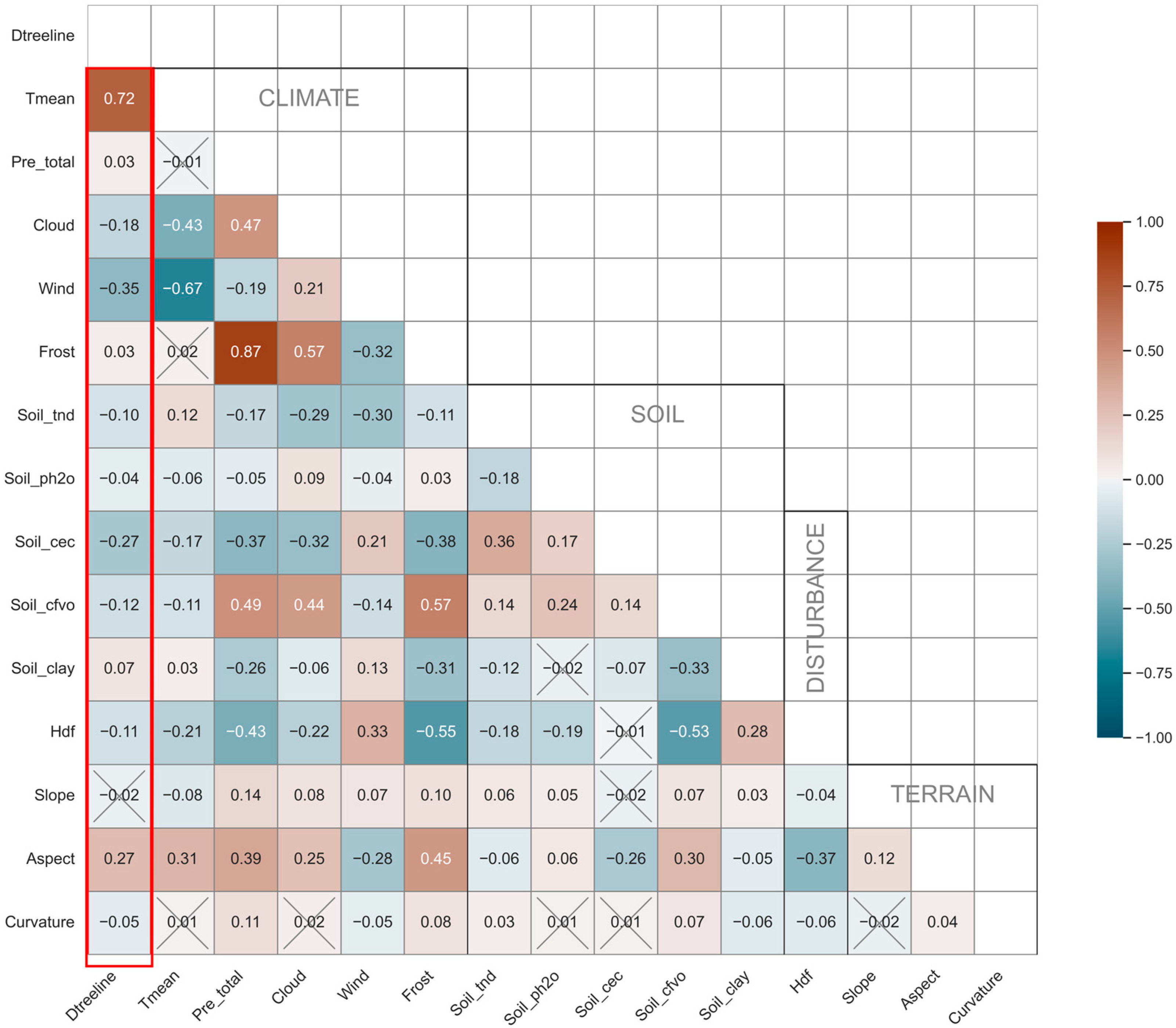
3.2. Correlation Analysis of Environmental Variables and Dtreeline

A significant correlation between Dtreeline and environmental variables can be observed (Figure 4). The highest correlation is with temperature (Tmean) at 0.72, which is statistically significant. Aside from Tmean, the correlations between Dtreeline and other environmental variables are low (absolute value up to 0.35). Dtreeline is positively correlated with Tmean, Pre_total, Frost, Soil_clay, and Aspect, meaning that higher values correspond to a larger Dtreeline. It is negatively correlated with Cloud, Wind, Soil_tnd, Soil_ph2o, Soil_cec, Soil_cfvo, Slope (not significant), and Curvature, though the Spearman correlation coefficient (ρ) values are small. There is a significant correlation between Pre_total and Frost (ρ = 0.87), and a relatively high correlation between Frost and Soil_cfvo (ρ = 0.57). To enhance the stability of the XGBoost model and reduce information redundancy, the Frost was removed in subsequent models.

3.3. The Importance Ranking of Key Environmental Variables

The optimal parameters for the XGBoost model were obtained through a grid search method with 10-fold cross-validation. The cross-validation method partitions the data, calculates the error for each partition, and derives a comprehensive error. The optimal parameters for XGBoost are ‘learning_rate’: 0.1, ‘max_depth’: 5, ‘n_estimators’: 1000. The model achieved an R2 value of 0.979, indicating high performance in fitting the 12 environmental variables and Dtreeline.
The ranking of importance from 12 different categories of environmental variables (excluding Tmean) to Dtreeline can reveal which environmental factors, besides temperature, most hinder the trees from reaching the theoretical treeline in the Yulong Snow Mountain region. Figure 5 shows the ranking of the importance of environmental variables to Dtreeline derived from the XGBoost model. Among these variables, the top three (annual total precipitation, wind speed, and anthropogenic disturbance) explain 46.17% of the spatial distribution of Dtreeline, with precipitation (20.6%) and wind speed (18.6%) having a significantly higher impact on Dtreeline than other factors. Among the climate impact factors, cloud cover (7%) ranks significantly lower than soil environmental factors. The total impact of soil factors on Dtreeline is 35.31%, with contributions ranked from highest to lowest as soil texture (clay content and mass fraction), coarse fragments (volumetric), cation exchange capacity at pH7, total nitrogen density, and soil pH in H2O. Notably, topographic environmental variables contribute the least to Dtreeline, explaining only 6.9% of its spatial variation. Among them, aspect contributes the most (5.6%), while curvature has almost no impact (0.2%). This means that topographic factors (slope, aspect, and curvature) have a minimal effect on the deviation of trees from the treeline position. Yulong Snow Mountain area, as the most popular outdoor activity spot, is affected by human activity (11.6%).
Partial Dependence Plots (PDP) demonstrate the average marginal effects of characteristics. For instance, as precipitation increases, higher Dtreeline is observed, while Wind and Hdf the opposite trend. There are threshold changes in the effects of annual precipitation and wind speed on Dtreeline, with significant randomness in the impact of Hdf on Dtreeline. We plotted 50 randomly selected Individual Conditional Expectation (ICE) plots for the top three main features (blue lines in Figure 5b,c) to show how Dtreeline changes for each sample at different values. Pre_total shows a markedly different effect (Figure 5b), with significant changes at two thresholds (810 mm/year and 970 mm/year). When precipitation is below 810 mm/year, increasing precipitation brings some actual tree lines closer to the thermal tree line. However, once precipitation exceeds 810 mm/year, its impact on the Dtreeline flattens. In some regions, the actual tree line is constrained by precipitation levels below 970 mm/year, but when precipitation surpasses 970 mm/year, the gap between the actual tree line and the thermal tree line widens quickly and then stabilizes. Increasing wind speed contributes to reducing Dtreeline values. However, when wind speed reaches 1.0 m/s, there is significant uncertainty in its impact on Dtreeline.

4. Discussion

4.1. What Constitutes the True Treeline and How Can It Be Determined?

A core issue is distinguishing the physiological causes for tree presence from random effects (disturbances and stand dynamics) in treeline research [3]. This is a challenging task [2], often leading to confusion between the fundamental niche boundary and the realized niche boundary [3,76]. Not all upper forest boundaries can be termed as treelines, and there is currently no universally accepted method for making this distinction. However, it is certain that the treeline should exclude factors such as intentional tree removal, earthquakes, landslides, and insect infestations that artificially lower the upper forest boundary. Yet, it is often difficult to accurately assess these situations. Therefore, we chose to train suitable models to aid in this determination. Our identification model yielded satisfactory results (Figure 2c,d, red dots). In this process, we introduced the feature variable of surface roughness (ULS), which refines the Digital Elevation Model (DEM) of the mountain with a tilted surface. This variable more accurately measures the actual elevation of mountain uplift or the actual depth of valley cutting at different terrace levels. In Southwest China, DEM gradually increases from southeast to northwest, forming a tilted surface. Using a uniform elevation threshold to judge the treeline is insufficient and may overlook the upper limit of trees at lower altitudes. We believe that the “ULS” can aid in treeline identification not only at the local scale but also in larger and more complex regions.

4.2. Why Does the Actual Treeline Sometimes Exceed the Thermal Treeline?

Most studies suggest that the actual treeline to be lower than the thermal treeline. In most real-world cases, this is true [8,9]. However, in this study, the treeline elevation on both the west and east sides of Yulong Snow Mountain is higher than the thermal treeline elevation. Trees may not reach the low-temperature limit due to certain obstacles, but there remains uncertainty as to why the treeline elevation exceeds the thermal treeline elevation.
This study speculates on several possible reasons for this phenomenon:
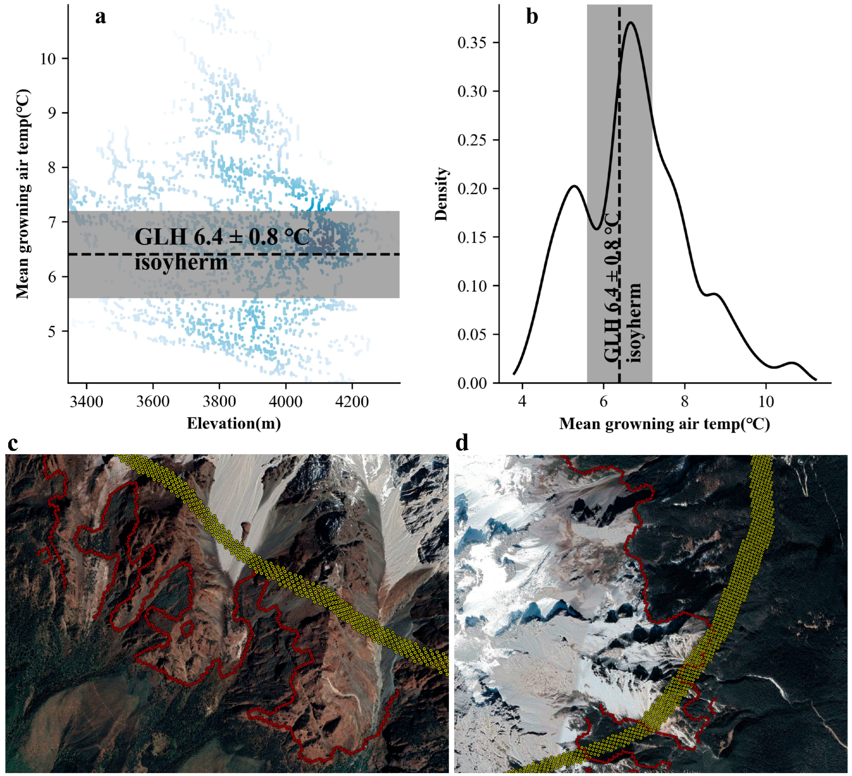
  • Water Vapor Channel: There might be a water vapor channel crossing the mountain from west to east along the left river, providing more water to trees on both sides. Google Maps reveals small canyon rivers on both sides of the actual treeline where it is higher than the thermal treeline.
  • Combined Effect of Water and Wind: The wind, formed along the canyons on both sides (narrow channel effect), has a higher speed, spreading tree seeds further and to higher elevations. The abundant water vapor in these canyons retains more solar radiation and surface reflection energy, reducing the low-temperature stress on seeds and facilitating sprouting.
  • Accuracy of Thermal Treeline Measurement: The thermal treeline, determined with a daily average temperature greater than 0.9 °C, is the best fitting result based on the Paulsen and Körner (2014) experiment but may lack absolute accuracy [3,5,7]. Therefore, the possibility that the actual treeline is higher than the thermal treeline exists.
In summary, while the spatial distribution patterns of the treeline and thermal treeline are similar, the variations in elevation on different sides of the mountain can be attributed to water availability, wind effects, and potential inaccuracies in thermal treeline measurements.

4.3. What Insights Does Ranking Key Environmental Factors Offer for Managing Alpine Environmental Issues?

Increasingly, studies are shifting from using the maximum altitude trees can reach as a response variable to using the actual and theoretical altitudes trees can attain [2,8]. Using Dtreeline as a response variable has its unique advantages: it highlights local variations that may be overlooked by emphasizing temperature too much. Moreover, as temperature conditions continue to be met, local environmental differences may become the decisive factor for whether the treeline ascends. Detailed studies of Dtreeline can better predict future trends in treeline changes. Our study found that temperature (Tmean) is the primary environmental factor affecting Dtreeline, with a strong correlation between the two (ρ = 0.87). This indicates that, currently, uneven heat distribution due to topography remains the main cause of Dtreeline. We hypothesize that in the near future, as temperatures continue to rise, only some treelines will ascend due to favorable temperature conditions.
Besides temperature, precipitation and wind speed are also important factors affecting Dtreeline. It is noteworthy that the correlation coefficients of precipitation and wind speed with Dtreeline are relatively low, at 0.03 and −0.35, respectively. However, in the ranking of variable importance, these two factors explain the spatial variability of the treeline the most. This indicates that the relationship between environmental variables and the treeline is likely nonlinear [8,77,78,79], with threshold effects. The local contribution analysis of the top three variables by XGBoost (Figure 5b,c) further supports this point. Many studies have found that the current strong trend in vegetation activity is due to worsening drought conditions, which cause the activity trend to decrease or even reverse [80]. Over the past 30 years, the correlation between vegetation activity and temperature has weakened, while the correlation with precipitation has increased. Therefore, the impact of environmental changes on treeline dynamics is complex and multidimensional. Further research into these nonlinear relationships will help better understand and predict future treeline changes.
Globally, the treeline on Yulong Snow Mountain, like other regions, is primarily limited by low temperature or insufficient moisture [9]. However, at the regional scale, the secondary influential factors differ compared to other studies. For instance, Wang et al. [2]. found that human interference is second only to moisture in importance for the Himalayan treeline, while Maher et al. [4] suggested that the elevation of the treeline in northern Alaska is more likely determined by local factors such as permafrost. In this study, wind speed also significantly affects the treeline. In the Hengduan Mountains, there are deep north–south-oriented gorges with significant canyon effects, which may amplify the impact of wind in such terrain. However, in this study, topographic factors (slope, aspect, and curvature) have minimal explanatory power for the spatial distribution of the treeline. Future research should use more representative indicators, such as the gully index and aspect index, to analyze the treeline distribution in this region.
There is a lag in the response of treelines to changes in environmental factors [3,81]. Our study primarily focuses on the distribution changes of treelines on Yulong Snow Mountain in 2019. Extracting environmental variables for a single year would introduce significant error. Therefore, we selected the annual average environmental variables over 20 years (2000 to 2019) to calculate the impact of environmental factors on the spatial distribution of treelines over a longer period. For calculating the growing season temperature, we used the number of days based on a threshold (0.9 °C) of daily surface temperature from 2000 to 2019. The growing season temperature was the average of 20 years of data, which helped mitigate the error caused by climate warming when calculating the temperatures of the growing season. However, our study has some limitations. The PDP and ICE plots for the top three variables (Figure 5b,d) show that the impact of individual variables on Dtreeline is limited and highly uncertain. The complex interaction of multiple factors may explain why treelines stabilize at certain elevations.
Our study found that, besides temperature, environmental factors such as precipitation and wind speed also significantly impact treeline distribution. This has important implications for managing changes in alpine ecological environments. First, management efforts should comprehensively consider factors such as temperature, precipitation, and wind speed, adopting a multidimensional perspective to address changes in alpine ecosystems. Second, the presence of nonlinear relationships and threshold effects suggests that management measures should be more flexible, adjusting strategies based on specific environmental conditions and changing trends. For example, in the context of climate warming, increasing attention to precipitation and wind speed can better protect alpine ecosystems. Finally, in-depth research into the nonlinear relationships between environmental factors will enhance the ability to predict changes in alpine ecological environments, providing a foundation for formulating scientifically sound management policies. Comprehensive analysis of various environmental factors and their interactions can more accurately assess the vulnerability and adaptive capacity of alpine ecosystems, leading to more effective protection measures.

5. Conclusions

This study employed the machine learning method SVM to delineate the upper limit of trees in the tree elevation distribution map based on LiDAR measurements. By computing the annual average growth season temperature using a threshold of 0.9 °C, Dtreeline was extracted, and its spatial pattern was observed. Utilizing the Spearman rank correlation, we explored the linear relationship between Dtreeline and environmental variables. Furthermore, XGBoost was employed to investigate the ranking of environmental variables, excluding temperature, in influencing the spatial interpretation of Dtreeline. Our research revealed that, in addition to temperature, precipitation and wind speed are also crucial. The impact of any single variable on spatial variation is limited and threshold dependent. In the context of ongoing global warming and the consequent reduction in low-temperature conditions, precipitation, particularly drought, may emerge as the predominant factor constraining the upward movement of trees. Fluctuations in treelines could result in the loss of endemic species in alpine cold temperate zones. Future research should prioritize the dynamics of mountain forests and alpine ecosystems, focusing on their sustainability and biodiversity. Understanding these aspects will be crucial for devising effective conservation strategies in the face of climate change.

Author Contributions

Conceptualization, C.L., R.Z., and Y.W.; data curation, L.Y.; formal analysis, C.L.; funding acquisition, Y.W.; methodology, C.L. and L.Y.; validation, T.Z. and Y.H.; visualization, Y.W.; writing—original draft, C.L.; writing—review and editing, Y.W. All authors have read and agreed to the published version of the manuscript.

Funding

This work was supported in part by the National Natural Science Foundation of China (Grant No. 42061004), in part by the Joint Special Project of Agricultural Basic Research of Yunnan Province (Grant No. 202101BD070001-093), and in part by the Youth Special Project of Xing Dian Talent Support Program of Yunnan Province (Grant No. XDYC-QNRC-2022-0230).

Data Availability Statement

Data are contained within the article.

Conflicts of Interest

The authors declare no conflicts of interest.

References

  1. Körner, C. Worldwide Positions of Alpine Treelines and Their Causes. In The Impacts of Climate Variability on Forests; Beniston, M., Innes, J.L., Eds.; Springer: Berlin/Heidelberg, Germany, 1998; pp. 221–229. [Google Scholar]
  2. Wang, X.; Xu, J.; Shen, Z.; Yang, Y.; Chen, A.; Wang, S.; Liang, E.; Piao, S. Enhanced Habitat Loss of the Himalayan Endemic Flora Driven by Warming-Forced Upslope Tree Expansion. Nat. Ecol. Evol. 2022, 6, 890–899. [Google Scholar] [CrossRef] [PubMed]
  3. Körner, C. The Cold Range Limit of Trees. Trends Ecol. Evol. 2021, 36, 979–989. [Google Scholar] [CrossRef] [PubMed]
  4. Maher, C.T.; Dial, R.J.; Pastick, N.J.; Hewitt, R.E.; Jorgenson, M.T.; Sullivan, P.F. The Climate Envelope of Alaska’s Northern Treelines: Implications for Controlling Factors and Future Treeline Advance. Ecography 2021, 44, 1710–1722. [Google Scholar] [CrossRef]
  5. Paulsen, J.; Körner, C. A Climate-Based Model to Predict Potential Treeline Position around the Globe. Alp. Bot. 2014, 124, 1–12. [Google Scholar] [CrossRef]
  6. Feng, L.; Tian, X.; El-Kassaby, Y.A.; Qiu, J.; Feng, Z.; Sun, J.; Wang, G.; Wang, T. Predicting Suitable Habitats of Melia azedarach L. In China Using Data Mining. Sci. Rep. 2022, 12, 12617. [Google Scholar] [CrossRef] [PubMed]
  7. Körner, C.; Paulsen, J. A World-Wide Study of High Altitude Treeline Temperatures. J. Biogeogr. 2004, 31, 713–732. [Google Scholar] [CrossRef]
  8. Case, B.S.; Buckley, H.L. Local-Scale Topoclimate Effects on Treeline Elevations: A Country-Wide Investigation of New Zealand’s Southern Beech Treelines. PeerJ 2015, 3, e1334. [Google Scholar] [CrossRef] [PubMed]
  9. Xie, Y.; Shen, Z.; Wang, T.; Malanson, G.P.; Peñuelas, J.; Wang, X.; Chen, X.; Liang, E.; Liu, H.; Yang, M.; et al. Uppermost Global Tree Elevations Are Primarily Limited by Low Temperature or Insufficient Moisture. Glob. Change Biol. 2024, 30, e17260. [Google Scholar] [CrossRef]
  10. Bader, M.Y.; Llambí, L.D.; Case, B.S.; Buckley, H.L.; Toivonen, J.M.; Camarero, J.J.; Cairns, D.M.; Brown, C.D.; Wiegand, T.; Resler, L.M. A Global Framework for Linking Alpine-Treeline Ecotone Patterns to Underlying Processes. Ecography 2021, 44, 265–292. [Google Scholar] [CrossRef]
  11. Greenwood, S.; Jump, A.S. Consequences of Treeline Shifts for the Diversity and Function of High Altitude Ecosystems. Arct. Antarct. Alp. Res. 2014, 46, 829–840. [Google Scholar] [CrossRef]
  12. Körner, C.; Hiltbrunner, E. Why Is the Alpine Flora Comparatively Robust against Climatic Warming? Diversity 2021, 13, 383. [Google Scholar] [CrossRef]
  13. Körner, C. Alpine Treelines: Functional Ecology of the Global High Elevation Tree Limits; Springer Science & Business Media: Berlin/Heidelberg, Germany, 2012; 229p. [Google Scholar]
  14. Huang, M.; Wang, G.; Bie, X.; Jiang, Y.; Huang, X.; Li, J.-J.; Shi, S.; Zhang, T.; Peng, P.-H. Seasonal Snow Cover Patterns Explain Alpine Treeline Elevation Better Than Temperature at Regional Scale. For. Ecosyst. 2023, 10, 100106. [Google Scholar] [CrossRef]
  15. Harsch, M.A.; Hulme, P.E.; McGlone, M.S.; Duncan, R.P. Are Treelines Advancing? A Global Meta-Analysis of Treeline Response to Climate Warming. Ecol. Lett. 2009, 12, 1040–1049. [Google Scholar] [CrossRef] [PubMed]
  16. Danby, R.K.; Hik, D.S. Responses of White Spruce (Picea glauca) to Experimental Warming at a Subarctic Alpine Treeline. Glob. Change Biol. 2007, 13, 437–451. [Google Scholar] [CrossRef]
  17. Davis, E.L.; Gedalof, Z.E. Limited Prospects for Future Alpine Treeline Advance in the Canadian Rocky Mountains. Glob. Change Biol. 2018, 24, 4489–4504. [Google Scholar] [CrossRef] [PubMed]
  18. Liang, E.; Wang, Y.; Eckstein, D.; Luo, T. Little Change in the Fir Tree-Line Position on the Southeastern Tibetan Plateau after 200 Years of Warming. New Phytol. 2011, 190, 760–769. [Google Scholar] [CrossRef]
  19. Singh, C.P.; Panigrahy, S.; Thapliyal, A.; Kimothi, M.M.; Soni, P.; Parihar, J.S. Monitoring the Alpine Treeline Shift in Parts of the Indian Himalayas Using Remote Sensing. Curr. Sci. 2012, 102, 559–562. [Google Scholar]
  20. Scott Armbruster, W.; Rae, D.A.; Edwards, M.E. Topographic Complexity and Terrestrial Biotic Response to High-Latitude Climate Change: Variance Is as Important as the Mean. In Arctic Alpine Ecosystems and People in a Changing Environment; Ørbæk, J.B., Kallenborn, R., Tombre, I., Hegseth, E.N., Falk-Petersen, S., Hoel, A.H., Eds.; Springer: Berlin/Heidelberg, Germany, 2007; pp. 105–121. [Google Scholar]
  21. Körner, C. The Use of ‘Altitude’ in Ecological Research. Trends Ecol. Evol. 2007, 22, 569–574. [Google Scholar] [CrossRef] [PubMed]
  22. Lindkvist, L.; Lindqvist, S. Spatial and Temporal Variability of Nocturnal Summer Frost in Elevated Complex Terrain. Agric. For. Meteorol. 1997, 87, 139–153. [Google Scholar] [CrossRef]
  23. Wang, T.; Zhang, Q.-B.; Ma, K. Treeline Dynamics in Relation to Climatic Variability in the Central Tianshan Mountains, Northwestern China. Glob. Ecol. Biogeogr. 2006, 15, 406–415. [Google Scholar] [CrossRef]
  24. Elliott, G.P.; Petruccelli, C.A. Tree Recruitment at the Treeline across the Continental Divide in the Northern Rocky Mountains, USA: The Role of Spring Snow and Autumn Climate. Plant Ecol. Divers. 2018, 11, 319–333. [Google Scholar] [CrossRef]
  25. Bråthen, K.A.; Fodstad, C.H.; Gallet, C. Ecosystem Disturbance Reduces the Allelopathic Effects of Empetrum hermaphroditum Humus on Tundra Plants. J. Veg. Sci. 2010, 21, 786–795. [Google Scholar] [CrossRef]
  26. Brown, D.G. Predicting Vegetation Types at Treeline Using Topography and Biophysical Disturbance Variables. J. Veg. Sci. 1994, 5, 641–656. [Google Scholar] [CrossRef]
  27. Byers, A.C. Historical and Contemporary Human Disturbance in the Upper Barun Valley, Makalu-Barun National Park and Conservation Area, East Nepal. Mt. Res. Dev. 1996, 16, 235–247. [Google Scholar] [CrossRef]
  28. Bader, M.Y.; van Geloof, I.; Rietkerk, M. High Solar Radiation Hinders Tree Regeneration above the Alpine Treeline in Northern Ecuador. Plant Ecol. 2007, 191, 33–45. [Google Scholar] [CrossRef]
  29. Germino, M.J.; Smith, W.K.; Resor, A.C. Conifer Seedling Distribution and Survival in an Alpine-Treeline Ecotone. Plant Ecol. 2002, 162, 157–168. [Google Scholar] [CrossRef]
  30. Bekker, M.F. Positive Feedback between Tree Establishment and Patterns of Subalpine Forest Advancement, Glacier National Park, Montana, U.S.A. Arct. Antarct. Alp. Res. 2005, 37, 97–107. [Google Scholar] [CrossRef]
  31. Liang, E.; Wang, Y.; Piao, S.; Lu, X.; Camarero, J.J.; Zhu, H.; Zhu, L.; Ellison, A.M.; Ciais, P.; Peñuelas, J. Species Interactions Slow Warming-Induced Upward Shifts of Treelines on the Tibetan Plateau. Proc. Natl. Acad. Sci. USA 2016, 113, 4380–4385. [Google Scholar] [CrossRef]
  32. Cieraad, E.; McGlone, M.S. Thermal Environment of New Zealand’s Gradual and Abrupt Treeline Ecotones. N. Z. J. Ecol. 2014, 38, 12. [Google Scholar]
  33. Amanda, H.; Jamie, S.; Paul, D.; Genia, H. A Review of Factors Controlling Southern Hemisphere Treelines and the Implications of Climate Change on Future Treeline Dynamics. Agric. For. Meteorol. 2023, 332, 109375. [Google Scholar]
  34. Dai, J.; Cui, H. A Review on the Studies of Alpine Timberline. Sci. Geogr. Sin. 1999, 19, 243–249. (In Chinese) [Google Scholar]
  35. Wang, Y.; Lu, X.; Zhu, H.; Liang, E. Field Survey and Research Approaches at Apine Treelines. Adv. Earth Sci. 2020, 35, 38–51. (In Chinese) [Google Scholar]
  36. Prakash Singh, C.; Mohapatra, J.; Pandya, H.A.; Gajmer, B.; Sharma, N.; Shrestha, D.G. Evaluating Changes in Treeline Position and Land Surface Phenology in Sikkim Himalaya. Geocarto Int. 2020, 35, 453–469. [Google Scholar] [CrossRef]
  37. Guo, D.; Zhang, H.-Y.; Hou, G.-L.; Zhao, J.-J.; Liu, D.-Y.; Guo, X.-Y. Topographic Controls on Alpine Treeline Patterns on Changbai Mountain, China. J. Mt. Sci. 2014, 11, 429–441. [Google Scholar] [CrossRef]
  38. Mathew, J.R.; Singh, C.P.; Solanki, H.; Mohapatra, J.; Nautiyal, M.C.; Semwal, S.C.; Singh, A.; Sharma, S.; Naidu, S.; Bisht, V.; et al. Improvement in the Delineation of Alpine Treeline in Uttarakhand Using Spaceborne Light Detection and Ranging Data. J. Appl. Remote Sens. 2023, 17, 022207. [Google Scholar] [CrossRef]
  39. Negi, P.S. Climate Change, Alpine Tree Line Dynamics and Associated Terminology: Focus on Northwestern Indian Himalaya. Trop. Ecol. 2012, 53, 371–374. [Google Scholar]
  40. Carlson, B.Z.; Corona, M.C.; Dentant, C.; Bonet, R.; Thuiller, W.; Choler, P. Observed Long-Term Greening of Alpine Vegetation—A Case Study in the French Alps. Environ. Res. Lett. 2017, 12, 114006. [Google Scholar] [CrossRef]
  41. Wang, Z.; Ginzler, C.; Eben, B.; Rehush, N.; Waser, L.T. Assessing Changes in Mountain Treeline Ecotones over 30 Years Using Cnns and Historical Aerial Images. Remote Sens. 2022, 14, 2135. [Google Scholar] [CrossRef]
  42. Nguyen, T.-A.; Kellenberger, B.; Tuia, D. Mapping Forest in the Swiss Alps Treeline Ecotone with Explainable Deep Learning. Remote Sens. Environ. 2022, 281, 113217. [Google Scholar] [CrossRef]
  43. Dubayah, R.; Blair, J.B.; Goetz, S.; Fatoyinbo, L.; Hansen, M.; Healey, S.; Hofton, M.; Hurtt, G.; Kellner, J.; Luthcke, S.; et al. The Global Ecosystem Dynamics Investigation: High-Resolution Laser Ranging of the Earth’s Forests and Topography. Sci. Remote Sens. 2020, 1, 100002. [Google Scholar] [CrossRef]
  44. Matasci, G.; Hermosilla, T.; Wulder, M.A.; White, J.C.; Coops, N.C.; Hobart, G.W.; Bolton, D.K.; Tompalski, P.; Bater, C.W. Three Decades of Forest Structural Dynamics over Canada’s Forested Ecosystems Using Landsat Time-Series and Lidar Plots. Remote Sens. Environ. 2018, 216, 697–714. [Google Scholar] [CrossRef]
  45. Wang, W.; Körner, C.; Zhang, Z.; Wu, R.; Geng, Y.; Shi, W.; Ou, X. No Slope Exposure Effect on Alpine Treeline Position in the Three Parallel Rivers Region, Sw China. Alp. Bot. 2013, 123, 87–95. [Google Scholar] [CrossRef]
  46. Wang, S.; He, Y.; Song, X. Impacts of Climate Warming on Alpine Glacier Tourism and Adaptive Measures: A Case Study of Baishui Glacier No. 1 in Yulong Snow Mountain, Southwestern China. J. Earth Sci. 2010, 21, 166–178. [Google Scholar] [CrossRef]
  47. Yuan, L.-l.; Wang, S.-j. Recreational Value of Glacier Tourism Resources: A Travel Cost Analysis for Yulong Snow Mountain. J. Mt. Sci. 2018, 15, 1446–1459. [Google Scholar] [CrossRef]
  48. Shaohua, Y.; Runguang, X.; Cui, C.; Chenggang, G.; Zhongzhi, X. Biodiversity Status and Conservation Strategies of Yulong Snow Mountain in Northwest Yunnan. Southwest China J. Agric. Sci. 2008, 863–869. (In Chinese) [Google Scholar] [CrossRef]
  49. Jianmeng, F.; Xiangping, W.; Chengdong, X.; Yuanhe, Y.; Jingyun, F. Distribution Pattern of Plant Species Diversity and Community Structure Along Altitude Gradient in Yulong Snow Mountain. J. Mt. Sci. 2006, 110–116. (In Chinese) [Google Scholar]
  50. Zhu, G.; Pu, T.; He, Y.; Shi, P.; Zhang, T.; Wei, W.; Niu, H. Characteristics of Inorganic Ions in Precipitation at Different Altitudes in the Yulong Snow Mountain, China. Environ. Earth Sci. 2013, 70, 2807–2816. [Google Scholar] [CrossRef]
  51. Danzeglocke, J. Remote Sensing of Upper Timberline Elevation in the Alps on Different Scales. In Proceedings of the 24th EARSeL Symp. New Strategies for European Remote Sensing, Dubrovnik, Croatia, 25–27 May 2004; pp. 25–27. [Google Scholar]
  52. Förster, M.; Schmidt, T.; Spindler, N.; Renner, K.; Wagner-Lücker, I.; Zebisch, M.; Neubert, M. Remote Sensing Methods to Monitor Habitats Potentially Threatened by Climate Change. In Proceedings of the Earth Resources and Environmental Remote Sensing/GIS Applications IV, Dresden, Germany, 23–26 September 2013; Michel, U., Civco, D.L., Schulz, K., Ehlers, M., Nikolakopoulos, K.G., Eds.; SPIE: Bellingham, WA, USA, 2013; p. 88930L. [Google Scholar]
  53. Zhou, R.; Ye, J.; Wang, Y. A Method and System for Constructing Rasterized Elevation Surface for Measuring Geomorphic Height Difference; Southwest Forestry University: Kunming, China, 2020. (In Chinese) [Google Scholar]
  54. Mu, H.; Li, X.; Wen, Y.; Huang, J.; Du, P.; Su, W.; Miao, S.; Geng, M. A Global Record of Annual Terrestrial Human Footprint Dataset from 2000 to 2018. Sci. Data 2022, 9, 176. [Google Scholar] [CrossRef]
  55. Kullman, L. Rapid Recent Range-Margin Rise of Tree and Shrub Species in the Swedish Scandes. J. Ecol. 2002, 90, 68–77. [Google Scholar] [CrossRef]
  56. Potapov, P.; Li, X.; Hernandez-Serna, A.; Tyukavina, A.; Hansen, M.C.; Kommareddy, A.; Pickens, A.; Turubanova, S.; Tang, H.; Silva, C.E.; et al. Mapping Global Forest Canopy Height through Integration of Gedi and Landsat Data. Remote Sens. Environ. 2021, 253, 112165. [Google Scholar] [CrossRef]
  57. Maimon, L.R.O. Machine Learning for Data Science Handbook: Data Mining and Knowledge Discovery Handbook; Springer International Publishing: Cham, Switzerland, 2023. [Google Scholar]
  58. Cortes, C.; Jackel, L.D.; Solla, S.; Vapnik, V.; Denker, J. Learning Curves: Asymptotic Values and Rate of Convergence. Adv. Neural Inf. Process. Syst. 1993, 6, 327–334. [Google Scholar]
  59. Hastie, T.; Tibshirani, R.; Friedman, J. Support Vector Machines and Flexible Discriminants. In The Elements of Statistical Learning; Springer: New York, NY, USA, 2009; pp. 417–458. [Google Scholar]
  60. Fu, Z.; Robles-Kelly, A.; Zhou, J. Mixing Linear Svms for Nonlinear Classification. IEEE Trans. Neural Netw. 2010, 21, 1963–1975. [Google Scholar] [PubMed]
  61. Zhang, X.; Zhou, J.; Liang, S.; Wang, D. A Practical Reanalysis Data and Thermal Infrared Remote Sensing Data Merging (Rtm) Method for Reconstruction of a 1-km All-Weather Land Surface Temperature. Remote Sens. Environ. 2021, 260, 112437. [Google Scholar] [CrossRef]
  62. Bentley, J.L. K-D Trees for Semidynamic Point Sets. In Proceedings of the Sixth Annual Symposium on Computational Geometry, Berkley, CA, USA, 7–9 June 1990; Association for Computing Machinery: New York, NY, USA, 1990; pp. 187–197. [Google Scholar]
  63. Ram, P.; Sinha, K. Revisiting Kd-Tree for Nearest Neighbor Search. In Proceedings of the 25th ACM SIGKDD International Conference on Knowledge Discovery & Data Mining, Anchorage, AK, USA, 4–8 August 2019; Association for Computing Machinery: New York, NY, USA, 2019; pp. 1378–1388. [Google Scholar]
  64. Qin, R.; Zhao, Z.; Xu, J.; Ye, J.-S.; Li, F.-M.; Zhang, F. Hrlt: A High-Resolution (1 Day, 1 km) and Long-Term (1961–2019) Gridded Dataset for Surface Temperature and Precipitation across China. Earth Syst. Sci. Data 2022, 14, 4793–4810. [Google Scholar] [CrossRef]
  65. Hengl, T.; Jesus, J.M.d.; Heuvelink, G.B.M.; Gonzalez, M.R.; Kilibarda, M.; Blagotić, A.; Shangguan, W.; Wright, M.N.; Geng, X.; Bauer-Marschallinger, B.; et al. Soilgrids250m: Global Gridded Soil Information Based on Machine Learning. PLoS ONE 2017, 12, e0169748. [Google Scholar] [CrossRef] [PubMed]
  66. Yang, K.; He, J.; Tang, W.; Lu, H.; Qin, J.; Chen, Y. China Meteorological Forcing Dataset (1979–2018); National Tibetan Plateau Data Center, Ed.; National Tibetan Plateau Data Center: Beijing, China, 2015. [Google Scholar]
  67. Wilson, A.M.; Jetz, W. Remotely Sensed High-Resolution Global Cloud Dynamics for Predicting Ecosystem and Biodiversity Distributions. PLoS Biol. 2016, 14, e1002415. [Google Scholar] [CrossRef]
  68. Farr, T.G.; Rosen, P.A.; Caro, E.; Crippen, R.; Duren, R.; Hensley, S.; Kobrick, M.; Paller, M.; Rodriguez, E.; Roth, L.; et al. The Shuttle Radar Topography Mission. Rev. Geophys. 2007, 45. [Google Scholar] [CrossRef]
  69. Dormann, C.F.; Elith, J.; Bacher, S.; Buchmann, C.; Carl, G.; Carré, G.; Marquéz, J.R.G.; Gruber, B.; Lafourcade, B.; Leitão, P.J.; et al. Collinearity: A Review of Methods to Deal with It and a Simulation Study Evaluating Their Performance. Ecography 2013, 36, 27–46. [Google Scholar] [CrossRef]
  70. Dormann, C.F.; McPherson, J.M.; Araújo, M.B.; Bivand, R.; Bolliger, J.; Carl, G.; Davies, R.G.; Hirzel, A.; Jetz, W.; Daniel Kissling, W.; et al. Methods to Account for Spatial Autocorrelation in the Analysis of Species Distributional Data: A Review. Ecography 2007, 30, 609–628. [Google Scholar] [CrossRef]
  71. MacFarland, T.W.; Yates, J.M. Spearman’s Rank-Difference Coefficient of Correlation. In Introduction to Nonparametric Statistics for the Biological Sciences Using R; MacFarland, T.W., Yates, J.M., Eds.; Springer International Publishing: Cham, Switzerland, 2016; pp. 249–297. [Google Scholar]
  72. Sedgwick, P. Spearman’s Rank Correlation Coefficient. BMJ 2014, 349, g7327. [Google Scholar] [CrossRef]
  73. Chen, T.; Guestrin, C. Xgboost: A Scalable Tree Boosting System. In Proceedings of the 22nd ACM SIGKDD International Conference on Knowledge Discovery and Data Mining, San Francisco, CA, USA, 13–17 August 2016; Association for Computing Machinery: New York, NY, USA, 2016; pp. 785–794. [Google Scholar]
  74. Zheng, Z.; Ma, Q.; Jin, S.; Su, Y.; Guo, Q.; Bales, R.C. Canopy and Terrain Interactions Affecting Snowpack Spatial Patterns in the Sierra Nevada of California. Water Resour. Res. 2019, 55, 8721–8739. [Google Scholar] [CrossRef]
  75. Ali, Z.A.; Abduljabbar, Z.H.; Taher, H.A.; Sallow, A.B.; Almufti, S.M. Exploring the Power of Extreme Gradient Boosting Algorithm in Machine Learning: A Review. Acad. J. Nawroz Univ. 2023, 12, 320–334. [Google Scholar]
  76. Paulsen, J.; Körner, C. Gis-Analysis of Tree-Line Elevation in the Swiss Alps Suggests No Exposure Effect. J. Veg. Sci. 2001, 12, 817–824. [Google Scholar] [CrossRef]
  77. Danby, R.K.; Hik, D.S. Variability, Contingency and Rapid Change in Recent Subarctic Alpine Tree Line Dynamics. J. Ecol. 2007, 95, 352–363. [Google Scholar] [CrossRef]
  78. Harsch, M.A.; Bader, M.Y. Treeline Form—A Potential Key to Understanding Treeline Dynamics. Glob. Ecol. Biogeogr. 2011, 20, 582–596. [Google Scholar] [CrossRef]
  79. Malanson, G.P. Complex Responses to Global Change at Alpine Treeline. Phys. Geogr. 2001, 22, 333–342. [Google Scholar] [CrossRef]
  80. Sun, M.; Sun, P. Climate-Driving Effects and Sustainbility of Vegetation Activity Change in Alpine and Subalpine Areas of Southwest China. Res. Soil Water Conserv. 2023, 30, 240–250. (In Chinese) [Google Scholar]
  81. Scheffer, M.; Carpenter, S.R.; Lenton, T.M.; Bascompte, J.; Brock, W.; Dakos, V.; van de Koppel, J.; van de Leemput, I.A.; Levin, S.A.; van Nes, E.H.; et al. Anticipating Critical Transitions. Science 2012, 338, 344–348. [Google Scholar] [CrossRef]
Figure 1. Location of Yulong Snow Mountain and the sampling area setup. We used a tree height map based on LiDAR measurements to filter out forest areas with tree heights greater than 3 m. Sampling areas were set every 3000 m along the upper edge of the forest to interpret the treelines within a 500 m range around each sampling area.
Forests 15 01261 g001
Figure 2. Figure illustrating the significant difference in elevation distribution and average growing season temperature (based on a 0.9 baseline) distribution between the actual treeline and the thermal treeline (6.4 ± 0.8 °C). (a) Scatter plot depicting the average growing season temperature of Treeline against altitude. (b) Density plot showing the distribution of average temperature during the growing season. (c,d) The display of actual and thermal treelines in Google Earth, with red dots representing actual treelines and yellow dots representing thermal treelines. In (c), the elevation of the thermal treeline is higher than the actual treeline, whereas in (d), the elevation of the thermal treeline is lower than the actual treeline.
Forests 15 01261 g002
Figure 3. Variations in the actual treeline, thermal treeline, and Dtreeline along latitude and longitude. Where there are two or more elevation values at the same longitude or latitude, a single value is obtained by averaging multiple values, then smoothing the curve through linear fitting. Dtreeline represents the difference between the actual and thermal treelines (blue area). (a). Variation with latitude. (b). Variation with longitude.
Forests 15 01261 g003
Figure 4. Correlogram depicting the relationships between Dtreeline and environmental variables. Each cell represents the Spearman correlation coefficient (ρ), with non-significant relationships indicated by a cross. The red frame highlights relationship between Dtreeline and environmental variables.
Forests 15 01261 g004
Figure 5. Result of the XGBoost for Dtreeline. (a) The relative importance of environmental variables in predicting the spatial variation of Dtreeline, error bars represent the standard deviation derived from the K-Fold cross-validation method (K = 10), indicating the variability in XGBoost model performance; (bd) ICE and PDP of the three most import variables: ICE (Individual Conditional Expectation) displayed the dependency relationships of each instance, represented by blue lines and PDP (Partial Dependence Plots) show the overall impact of a feature on the target variable, i.e., the average dependency relationship, represented by orange lines.
Forests 15 01261 g005
Table 1. Features for the treeline recognition model.
VariableDescriptionResolution
DEMElevation30 m
VDDVertical distance between the point and the highest point30 m
LDDHorizontal distance between the point and the highest point30 m
ULSThe degree of uplift or depression in the location250 m
HFPThe degree of interference from human activities1 km
Table 2. Descriptions of environmental variables used for XGBoost. There were 14 variables in total.
VariableDescriptionUnitsYearResolutionSource
TmeanDaily average temperature°C2000–20191000 m[61]
Pre_totalTotal precipitation over a specific period of timemm/year2000–20191000 m[64]
CloudMean annual cloud frequency%2000–20141000 m[67]
WindMagnitude of the two-dimensional horizontal air velocity near the surfacem/s2000–20181000 m[66]
FrostNumber of days where the daily maximum temperature is below 0 °Cdays2000–20191000 m[64]
Soil_tndTotal nitrogen densityg m−2 250 m[65]
Soil_ph2oSoil pH in H2O _ 250 m[65]
Soil_cecCation exchange capacity at pH7mmol(c)/kg 250 m[65]
Soil_cfvoCoarse fragments (volumetric)Per 10000 250 m[65]
Soil_claySoil texture (clay content and mass fraction)% 250 m[65]
HdfAnthropogenic disturbance_2010–20191000 m[54]
SlopeThe steepness of the terrain surfacedegree 30 m[68]
AspectThe orientation or direction that a slope faces_ 30 m[68]
CurvatureThe rate of change in the direction of a slope_ 30 m[68]
Table 3. Confusion matrix of the SVM model.
PositiveNegative
Positive88776
Negative158429
Disclaimer/Publisher’s Note: The statements, opinions and data contained in all publications are solely those of the individual author(s) and contributor(s) and not of MDPI and/or the editor(s). MDPI and/or the editor(s) disclaim responsibility for any injury to people or property resulting from any ideas, methods, instructions or products referred to in the content.

