Spatial and Temporal Variations of Vegetation Phenology and Its Response to Land Surface Temperature in the Yangtze River Delta Urban Agglomeration

Abstract

In the Yangtze River Delta urban agglomeration, which is the region with the highest urbanization intensity in China, the development of cities leads to changes in land surface temperature (LST), while vegetation phenology varies with LST. To investigate the spatial and temporal changes in vegetation phenology and its response to LST in the study area, this study reconstructed the time series of the enhanced vegetation index (EVI) based on the MODIS EVI product and extracted the vegetation phenology indicators in the study area from 2002 to 2020, including the start of the growing season (SOS), the end of the growing season (EOS), and the growing season length (GSL), and analyzed the temporal–spatial patterns of vegetation phenology and LST in the study area, as well as the correlation between them. The results show that (1) SOS was advanced, EOS was postponed, and GSL was extended in the study area from 2002 to 2020, and there were obvious differences in the vegetation phenology indicators under different land covers and cities; (2) LST was higher in the southeast than in the northwest of the study area from 2002 to 2020, with an increasing trend; and (3) there are differences in the response of vegetation phenology to LST across land covers and cities, and SOS responds differently to LST at different times of the year. EOS shows a significant postponement trend with the annual mean LST increase. Overall, we found differences in vegetation phenology and its response to LST under different land covers and cities, which is important for scholars to understand the response of vegetation phenology to urbanization.

1. Introduction

The rapid development of human society and economy has led to accelerated urbanization and continuous changes in the global climate [1,2]. As a result, the environment of urban areas has been greatly affected, including urban heat stress, urban pollution, and urban ecological changes [3]. One of these effects is the increase in land surface temperature (LST) [4]. With the changes in LST, corresponding changes in vegetation phenology in these areas are induced, which in turn affects the energy, carbon, and water cycles; vegetation dynamics; and public health, among others [5,6,7,8,9].

Vegetation phenology is the seasonal timing of plant growth and reproduction such as budding, leaf development, flowering, fruiting, yellowing, and so on, and is influenced by a combination of environmental factors such as the climate, hydrology, soil, and human activities [10,11,12,13]. Vegetation phenology is highly sensitive to environmental change, and it can also regulate climate by altering the exchange of energy, water, and carbon between the land surface and the atmosphere [14,15,16]. With the emergence of global warming, a large number of scholars have found that vegetation phenology changes with temperature, and the main trend is that as the temperature increases, the start of the growing season (SOS) is advanced, the end of the growing season (EOS) is delayed, and the growing season length (GSL) is extended [17,18,19,20].

The changes in the underlying surface in urban construction, especially the increase in impervious surfaces and buildings made of asphalt, cement, and other materials, lead to an increase in the temperature in these areas [21]. Scholars have conducted a lot of research on the impact of urbanization on vegetation phenology, which mainly focuses on the changes in LST and vegetation phenology in cities and the surrounding areas due to the intensity of urbanization, urban–rural differences, and so on. Some scholars found that the effect of urban climate on vegetation phenology decayed exponentially with distance from urban areas [22]; others found that the effect of urbanization on phenology is related to LST [23]. Many of these studies have shown that the changes in LST are closely related to the changes in vegetation phenology and that vegetation phenology responds differently to LST in different cities [24]—SOS and EOS tend to change as the LST rises [5,23,24,25]. At the same time, the temperature sensitivity of vegetation phenology tends to decrease with increasing LST, such as when LST increases; changes in vegetation phenology in areas with higher LST tend to be less pronounced than changes in areas with lower LST [26]. In addition, due to inter-city heterogeneity, there are some differences in the vegetation phenology of different cities [27]. However, there may be similar differences in the response of vegetation phenology to environmental factors under different land covers [28]. Previous studies have estimated that vegetation phenology in China can be affected by cities over an area of up to 20 km [29] and that these areas may encompass a wide range of different land covers. Meanwhile, previous studies on urban vegetation phenology have focused on the urban–rural gradient, whereas urban agglomerations, as areas with a large concentration of population and economy, are bound to have an impact on vegetation phenology due to the strong human activities within them and the expansion of the city limits, which cannot be ignored. Therefore, it is necessary to conduct an analysis from the perspective of different land covers and cities within the urban agglomerations. By studying LST and vegetation phenology under different land covers and cities, we can reveal the changing pattern and response relationship between vegetation phenology and LST in different land covers and cities and help residents better cope with urbanization and environmental changes.

In summary, vegetation phenology often responds to changes in LST, and changes in LST and vegetation phenology, as well as the response of vegetation phenology to LST, may vary under different land covers and different cities. We aimed to analyze the changes in LST, vegetation phenology, and the response of vegetation phenology to LST for different land covers and different cities in the Yangtze River Delta urban agglomeration from 2002 to 2020. We extracted vegetation phenology indicators (SOS, EOS, and GSL) for the Yangtze River Delta urban agglomeration from enhanced vegetation index (EVI) data. We combined phenological indicators with LST data to explore (1) the spatial and temporal changes in vegetation phenology and LST of different land covers and different cities in the Yangtze River Delta urban agglomeration during 2002–2020 and (2) the response of vegetation phenology to LST under different land covers and different cities.

2. Materials and Methods

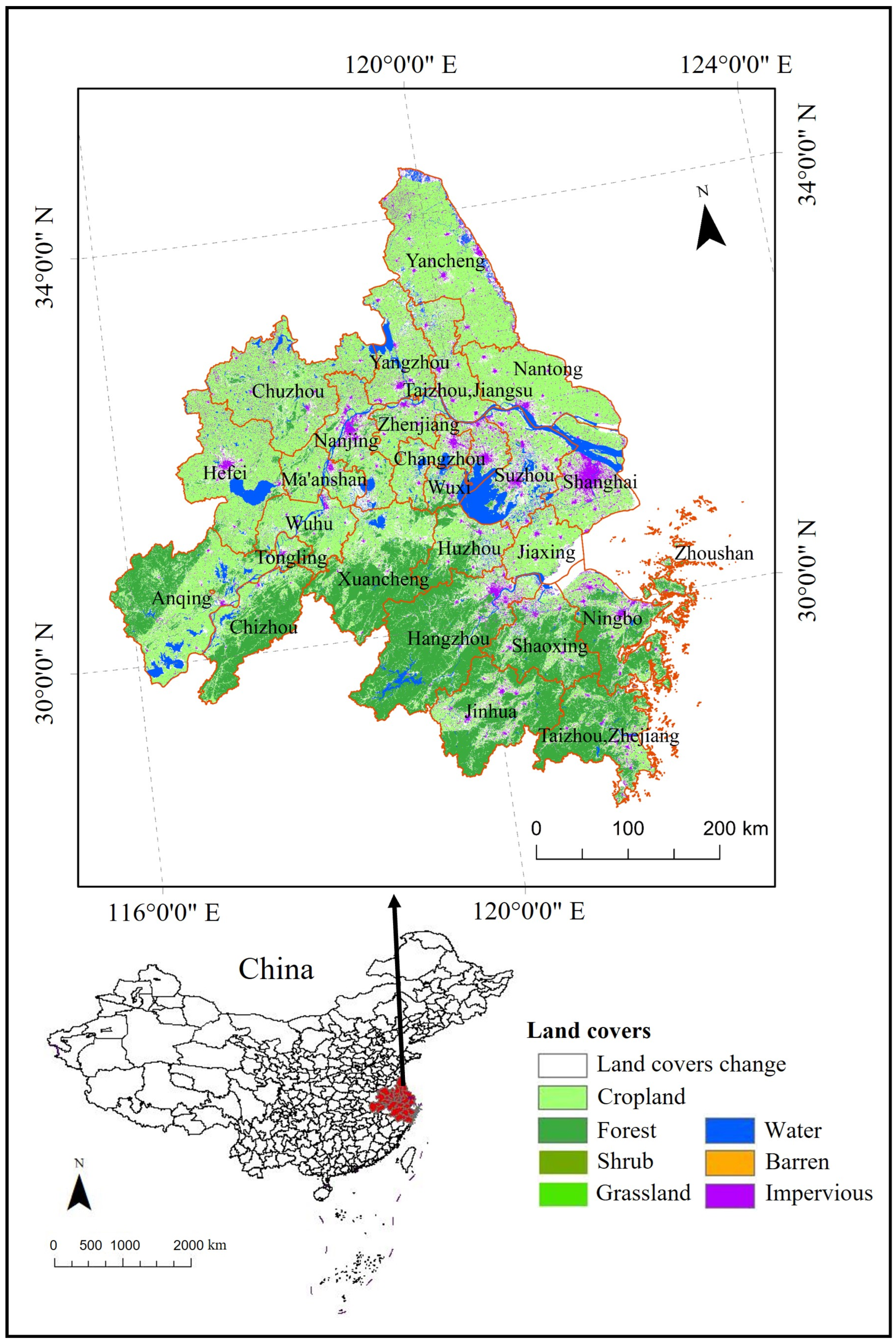
2.1. Study Area

The Yangtze River Delta Urban Agglomeration (29°20′–32°34′ N, 115°46′–123°25′ E), located in the lower reaches of the Yangtze River Basin, on the west coast of the Pacific Ocean, has a well-developed regional economy. The area includes 26 cities—Shanghai; Nanjing, Wuxi, Changzhou, Suzhou, Nantong, Yancheng, Yangzhou, Zhenjiang, and Taizhou in Jiangsu Province; Hangzhou, Ningbo, Jiaxing, Huzhou, Shaoxing, Jinhua, Zhoushan, and Taizhou in Zhejiang Province; and Hefei, Wuhu, Ma’anshan, Tongling, Anqing, Chuzhou, Chizhou, and Xuancheng in Anhui Province. The climate is predominantly subtropical monsoon, warm, and humid all year round; the average annual temperature is 15–17 °C, and the average annual precipitation is about 1000–1800 mm. The main crops are rice, winter wheat, and maize. Forest vegetation types are mainly mixed evergreen deciduous broad-leaf forests, green broad-leaved forests, and temperate deciduous broad-leaved forests. The land cover in the northern part of the study area is dominated by cropland and the southern part is dominated by forests, while large areas of impervious surfaces still exist in cities such as Shanghai, Nanjing, Suzhou, etc. The land cover in the entire study area is mainly composed of three types: cropland (46.38%), forests (26.70%), and impervious surfaces (6.31%), and the other types (water is not taken into account) are very few and can be ignored (Figure 1).

2.2. Data

2.2.1. EVI Data

Enhanced vegetation index data were obtained from MOD13Q1 vegetation index data provided by the National Aeronautics and Space Administration (NASA), which contains both normalized difference vegetation index (NDVI) and EVI data, and we extracted phenology indicators from the EVI data. Compared to NDVI data, EVI data not only removes the influence of the vegetation canopy background but also reduces the influence of atmospheric and soil noise and mitigates the oversaturation problem of NDVI [30]; it is more sensitive to changes in dense vegetation [31]. The data have a temporal resolution of 16d and a spatial resolution of 250 m. We used the data from 2001 to 2021, in which the Yangtze River Delta urban agglomeration covered four image strips, thus containing a total of 1932 images for 21 years (the extraction of vegetation phenology indicators requires the extraction of vegetation phenology parameters for the intermediate year using at least three consecutive years of vegetation index data; for example, extracting vegetation phenology indicators for 2002 requires the use of vegetation index data for 2001–2003.

2.2.2. LST Data

We considered the following two factors: (1) LST is closely related to both urbanization and vegetation phenology [8,32,33]; (2) urban ecosystems are affected by both global warming and urbanization compared to natural ecosystems, and in previous studies of vegetation phenology, atmospheric temperature was more often used to reflect changes in background climate due to global warming, whereas LST was more often used to reflect changes in temperature due to urbanization because of the significant impact of changes in the subsurface caused by urbanization [34]. Therefore, we used LST data instead of atmospheric temperature data. The LST data used comprised a daily 1 km all-weather land surface temperature dataset for China’s landmass and its surrounding areas (TRIMS LST; 2000–2022) [35,36,37,38]. The dataset was prepared following an enhanced satellite thermal infrared remote sensing–reanalysis data integration method. The data are an all-weather high-quality LST dataset with good precision and quality, having a high agreement with the daily 1 km Terra/Aqua MODIS LST product, which is now widely used in academia every day. The difference between clear-sky and non-clear-sky conditions is not significant. The mean bias deviation (MBD) of the dataset is 0.09 K and 0.03 K, and the standard deviation of bias (STD) is 1.45 K and 1.17 K for daytime and nighttime when using MODIS LST as a reference. The spatial resolution is 1 km and seamless, and the temporal resolution is 4 times a day throughout 2000–2021—of which we use the data from 2001 to 2020—and the data of each year are divided into four periods: the winter (including December of the previous year and January and February of the current year), March, April, and the annual mean because previous studies have shown that the SOS response is more pronounced in winter and spring temperatures [39,40]; additionally, considering that SOS in the study area occurs mainly before May, the response of SOS to May temperatures is negligible, whereas EOS occurs later and may be affected by year-round temperatures [27]. Using LST data from different time periods, we analyze the response of SOS to winter, March, and April LSTs and the response of EOS to the annual average LST.

2.2.3. Precipitation Data

We used precipitation data—a new daily gridded precipitation dataset for the Chinese mainland based on gauge observations [41,42,43]. The dataset is based on daily precipitation observations at the station and is prepared by applying monthly precipitation constraints and topographic corrections based on the idea of precipitation background field and precipitation ratio field construction. The dataset precision and quality are good and in good agreement with currently used precipitation datasets (CGDPA, CN05.1, and CMA V2.0). The spatial variability of precipitation can be better characterized. The median correlation coefficient between the daily valued time series of the dataset and the daily valued precipitation observations at the high-density sites was 0.78, the median root-mean-square error (RMSE) was 8.8 mm/d, and the median Kling–Gupta efficiency (KGE) value was 0.69. The spatial resolutions are 0.1°, 0.25°, and 0.5°, and the temporal resolution is 1 time per day, of which we used the 2001–2020 data with a spatial resolution of 0.1°. Similar to the LST data, we also divided the precipitation data for each year into four time periods—winter, March, April, and the annual mean.

2.2.4. Land Cover Data

We used land cover data—the 30 m annual land cover datasets and dynamics in China from 1985 to 2022 [44]. The data are based on satellite image data, China land use/cover datasets, third-party validation data, and existing year-by-year land use/cover data, and are obtained through a series of processes, such as the generation of training and test samples, the construction of yearly input features, the checking of classifications and spatial and temporal consistency, the assessment of accuracy, and the comparison of products. The overall precision is 76.45% < overall accuracy (OA) < 82.51%, with an average OA of 79.30 ± 1.99%. The data are better than MCD12Q1 and ESACCI_LC in terms of overall precision for all years. The data span the period of 1985–2021 with a spatial resolution of 30 m and a temporal resolution of 1 year. We used data from 2002 to 2020 in it.

2.3. Methodology

We explored the response of vegetation phenology to LST using the proposed framework in Figure 2. Firstly, we collected and preprocessed datasets from different years, including EVI data, land cover data, and LST data; secondly, we extracted the vegetation phenology indicators SOS, EOS, and GSL from the EVI data; thirdly, we used these datasets to analyze the spatial and temporal patterns of vegetation phenology and LST and the correlation between vegetation phenology and LST in different cities and different land covers.

2.3.1. Reconstruction of Vegetation Index Time Series

Although the MOD13Q1 data have been subjected to noise rejection, data acquired through remote sensing are inevitably affected by the sensors themselves, as well as by atmospheric aerosols and clouds, resulting in a reduction in the precision of the data. Therefore, we need to reconstruct the vegetation index time series as well as smoothing. Commonly used methods for vegetation index time series reconstruction include the adaptive Savitzky–Golay filtering (S-G) [45], the fits to asymmetric Gaussians (A-G) [46], the double Logistic function [47], and so on.

It was found that the A-G fitting algorithms not only generate more consistently reconstructed NDVI time series to the original NDVI temporal curve, but also perform extremely similarly to keep the fidelity of high-quality NDVI samples, and their fitting NDVI series are better [48]. Therefore, we used the A-G method to reconstruct the vegetation index time series. Firstly, we extracted the values of all remotely sensed images for a given year at the same location. Then, we fitted the values at that location using the A-G method to obtain a continuous time series curve for one year at that location.

The method fits the vegetation data with a local model function based on the interval between the maximum and minimum values in the time series. The local model function is as follows:

$$f\left(\mathrm{t}\right)=f\left(\mathrm{t};\mathrm{c},\mathrm{m}\right)=\mathrm{a}+\mathrm{b}g\left(\mathrm{t};\mathrm{m}\right)$$

(1)

where the base level and the amplitude are determined by the linear parameters c = (a, b) and the shape of the basis function g(t, m) is determined by the nonlinear parameters m = (m₁, m₂, …, m_n). The basis function of the asymmetric Gaussian function is:

$$g\left(\mathrm{t};{\mathrm{m}}_1,{\mathrm{m}}_2,\dots ,{\mathrm{m}}_5\right)=\left\{\begin{array}{c}\exp \left[-{\left({\displaystyle \frac{\mathrm{t}-{\mathrm{m}}_1}{{\mathrm{m}}_2}}\right)}^{{\mathrm{m}}_3}\right]\mathrm{t}>{\mathrm{m}}_1\\ \exp \left[-{\left({\displaystyle \frac{\mathrm{t}-{\mathrm{m}}_1}{{\mathrm{m}}_4}}\right)}^{{\mathrm{m}}_5}\right]\mathrm{t}<{\mathrm{m}}_1\end{array}\right.$$

(2)

where m₁ is used to determine the position of the maximum or minimum for the independent time variable t; m₂ and m₃ determine the width and flatness (kurtosis) of the right function half; and m₄ and m₅ determine the width and flatness of the left half. The time series in the whole time interval [t_L, t_R] is modelled using the global function F(t), F(t) is

$$F\left(\mathrm{t}\right)=\left\{\begin{array}{c}\alpha \left(\mathrm{t}\right)f_{\mathrm{L}}\left(\mathrm{t}\right)+\left[1-\alpha \left(\mathrm{t}\right)\right]f_{\mathrm{C}}\left(\mathrm{t}\right){\mathrm{t}}_{\mathrm{L}}<\mathrm{t}<{\mathrm{t}}_{\mathrm{C}}\\ \beta \left(\mathrm{t}\right)f_{\mathrm{C}}\left(\mathrm{t}\right)+\left[1-\beta \left(\mathrm{t}\right)\right]f_{\mathrm{R}}\left(\mathrm{t}\right){\mathrm{t}}_{\mathrm{C}}<\mathrm{t}<{\mathrm{t}}_{\mathrm{R}}\end{array}\right.$$

(3)

where α(t) and β(t) are cut-off functions that in small intervals around (t_L + t_C)/2 and (t_C + t_R)/2, respectively, smoothly drop from 1 to 0. f_L(t), f_C(t), and f_R(t) are local model functions fitted to the left minimum, the central maximum, and the right minimum, respectively, and are located in the interval [t_L, t_R]. By merging local functions into global functions, it is possible to ensure that the fitting function follows the time series while increasing flexibility [46].

2.3.2. Extraction of Vegetation Phenology Indicators

It was found that vegetation phenology indicators derived from MODIS vegetation index data were in good agreement with field observations in terms of absolute errors and time trends [49,50]. The vegetation phenology indicators we used were SOS, EOS, and GSL. Common methods used in previous studies to extract these indicators include thresholding, curve fitting, maximum rate of change, and so on.

Among them, the dynamic threshold method within the threshold method has better adaptability, and considering that the EVI in the city is lower compared with that in the countryside, the use of the fixed threshold method will lead to errors in the obtained phenological indicators, and previous studies have shown that the vegetation phenology extracted using the dynamic threshold method is consistent with the time recorded at the observatory [51]. Therefore, we adopted the dynamic threshold method to extract vegetation phenology parameters; that is, the time when the fitted curves on the left and right sides reached a certain proportion of the seasonal amplitude was taken as SOS and EOS, respectively, and the difference between EOS and SOS was taken as GSL. When scholars initially proposed the dynamic threshold method, they suggested that the SOS and EOS thresholds be set at about 20% of the annual amplitude of the NDVI [46]; in other studies, scholars adopted 20% as the thresholds for SOS and EOS based on previous experience when studying the vegetation phenology of 32 major Chinese cities [23]. When studying the climatic changes in a typical vegetation sample area of the northern Tibetan Plateau, the SOS threshold was set at 10% and the EOS threshold at 20% based on previous experience and a large number of experiments [52]. In the study of vegetation climate change in Zhejiang Province, based on the characteristics of high vegetation cover and incomplete symmetry of vegetation growth curves in Zhejiang Province, the SOS threshold was set at 30% and the EOS threshold at 15% on the basis of a large number of experiments [51]. In conclusion, it is more flexible in using the dynamic threshold method to extract vegetation phenology parameters. Considering that Zhejiang Province is located in the southern part of the study area, with large forested areas and high vegetation coverage, this paper adopts the thresholds set by scholars in extracting the vegetation phenology in Zhejiang Province, with 30% as the SOS threshold and 15% as the EOS threshold for extracting the phenology indicators. Since the vegetation phenology indicators extracted from remotely sensed data may go beyond the range of vegetation physiological periods and lead to errors, to eliminate the uncertainty caused by these errors, the SOS and EOS were limited to 50–180 days and 240–330 days, respectively.

2.3.3. Methods of Statistical Analyses

• Partial correlation analysis

Since temperature and precipitation are two important influences on vegetation phenology, and the effect of precipitation cannot be ignored in the analysis of vegetation phenology, we analyzed the correlation between vegetation phenology and LST after excluding the precipitation factor by partial correlation analysis, with the following formula:

$$c_{yx\times z}={\displaystyle \frac{c_{yx}-c_{yz}{c}_{xz}}{\sqrt{\left(1-c_{yz}^2\right)\left(1-c_{xz}^2\right)}}}$$

(4)

where $c_{yx\times z}$ is the partial correlation coefficient between y and x after the control variable z, $c_{yx}$ is the correlation coefficient between y and x, y is the vegetation phenology indicators, x is LST, and z is precipitation.

2.

Geographical weighted regression analysis (GWR)

3.

Considering the spatial heterogeneity in the response of vegetation phenology to LST, we used GWR to analyze the spatial differences in the response of vegetation phenology to LST, with the following formula:

$$y_i={\beta }_0\left({\mu }_i,{\nu }_i\right)+\sum _{k=1}^p{\beta }_k\left({\mu }_i,{\nu }_i\right)x_{ik}+{\epsilon }_i\left(i=1,2,3,\cdots ,n\right)$$

(5)

where $y_i$ represents the vegetation phenology indicators of raster i, ${\beta }_0$ is the intercept, $\left({\mu }_i,{\nu }_i\right)$ is the coordinate of raster i, k is the number of independent variables, ${\beta }_k$ is the regression coefficient of the kth independent variable, $x_{ik}$ is the kth independent variable of raster i, and ${\epsilon }_i$ is the random error.

3. Results

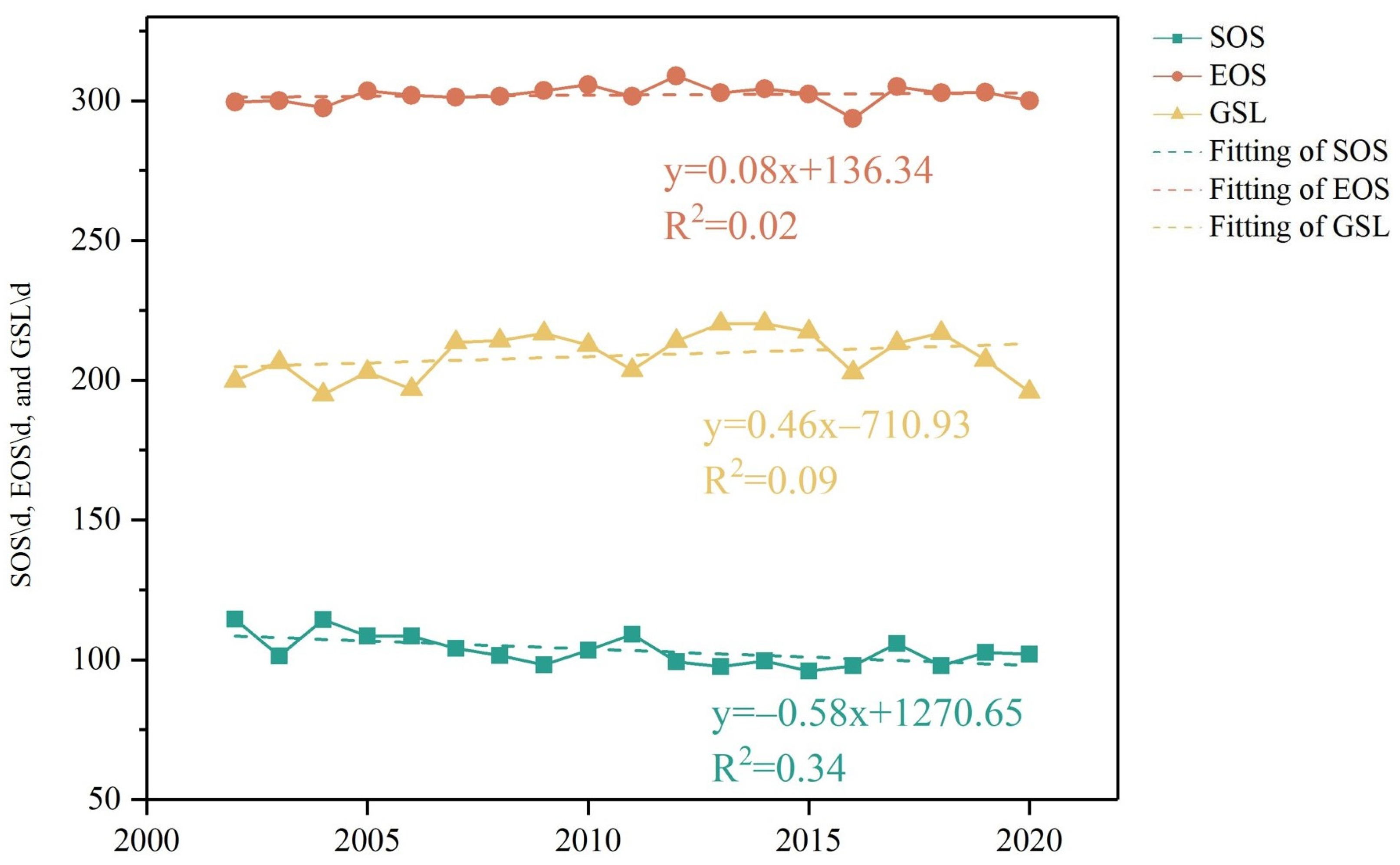
3.1. Spatial and Temporal Patterns of Vegetation Phenology

We extracted the main vegetation phenology indicators of the Yangtze River Delta urban agglomeration from 2002 to 2020, that is, SOS, EOS, and GSL, by fitting the EVI time series curves using the A-G method with a threshold of 30% for SOS and 15% for EOS. The results showed that the mean value of SOS in the study area from 2002 to 2020 was 7.64 days, the mean value of EOS was 294.47 days, and the GSL mean value was 206.77 days.

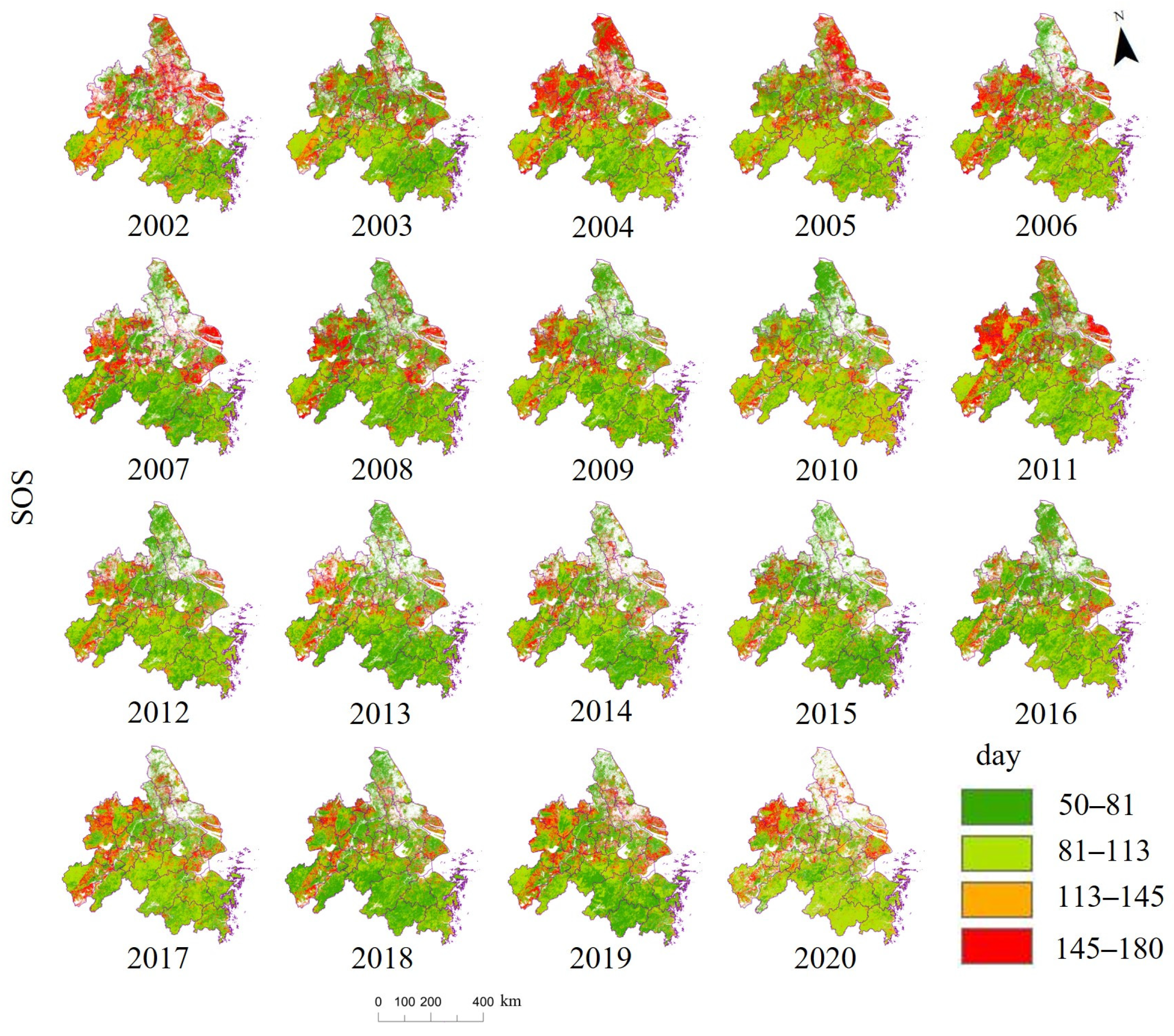
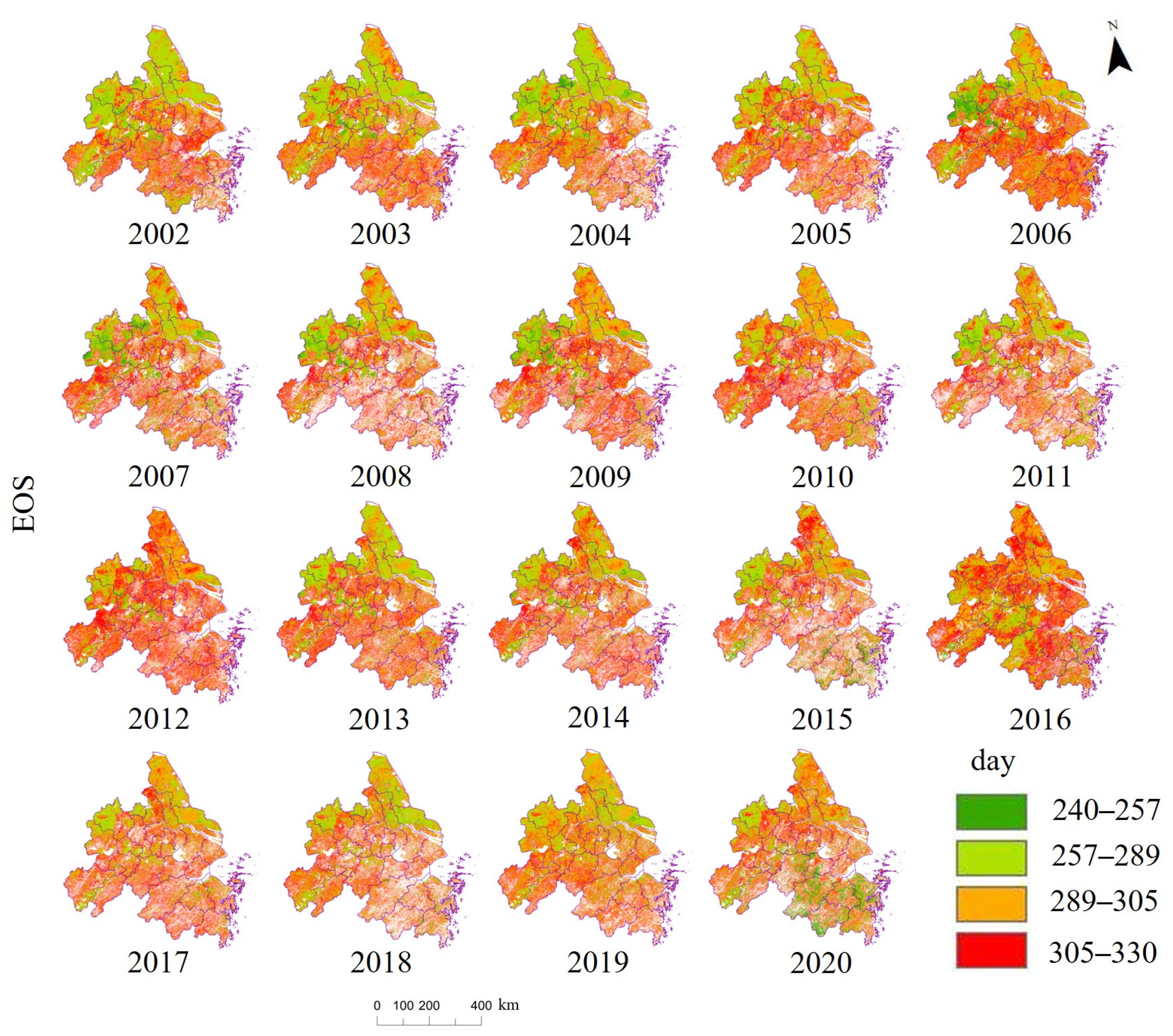
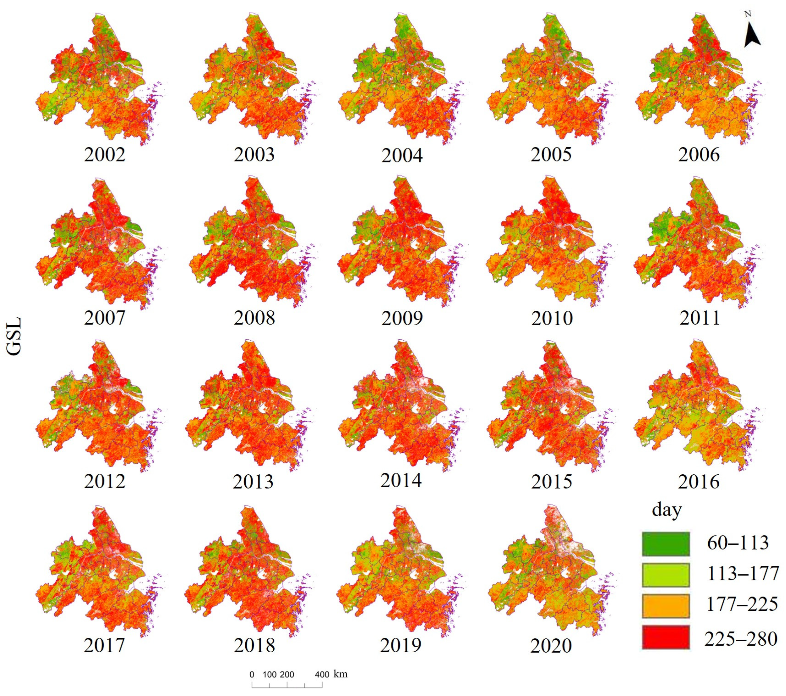
3.1.1. Spatial and Temporal Characteristics of Vegetation Phenology in the Study Area

Figure 3, Figure 4 and Figure 5 show the summary statistics for vegetation phenology in the Yangtze River Delta urban agglomeration from 2002 to 2020. SOS is earliest in the area of concentrated impervious surfaces and forests in the southeast, followed by cropland in the north of Xuancheng and Huzhou and forests in the southwest of the study area, and latest in the east and west along the river basins and cropland distributed around impervious surfaces; SOS is significantly earlier than the surrounding areas in areas where impervious surfaces are concentrated (Figure 3). EOS is earliest in the northwestern and western river basins of the study area, followed by the northern cropland, and latest in the south-central and especially in the southern forest areas, which are similar to SOS, and the phenomenon of EOS is seen to occur later in the areas of impervious surface concentrations than in the surrounding areas (Figure 4). The GSL is the shortest in the northwest and in the east and west along the river basin it is shorter and longer in areas of concentrated impervious surfaces and in southern forested areas; similarly, the GSL shows longer characteristics in the concentrated areas of impervious surfaces than in the surrounding areas (Figure 5). Vegetation phenology in the concentrated area of impervious surfaces showed obvious differences compared to the surrounding areas; meanwhile, SOS was significantly delayed in the cropland surrounding the concentrated area of impervious surfaces compared to the cropland in other areas, and they became the two extremes of the earliest and the latest SOS. The reason for this phenomenon may be due to the fact that areas of concentrated impervious surfaces tend to have higher LSTs compared to other areas, and the increased LSTs lead to significant changes in vegetation phenology.

Figure 6 shows the trends in vegetation phenology from 2002 to 2020—SOS in the study area showed an overall advance trend of −0.58 days per year; EOS showed an overall delayed trend, which was smaller than SOS, with a change of only 0.08 days per year; and GSL showed an overall lengthening trend, with a change of 0.46 days per year. The three indicators of vegetation phenology showed a certain degree of fluctuation, with SOS showing local maximums in 2011 and 2017, while EOS and GSL showed local minimums in 2011 and 2016.

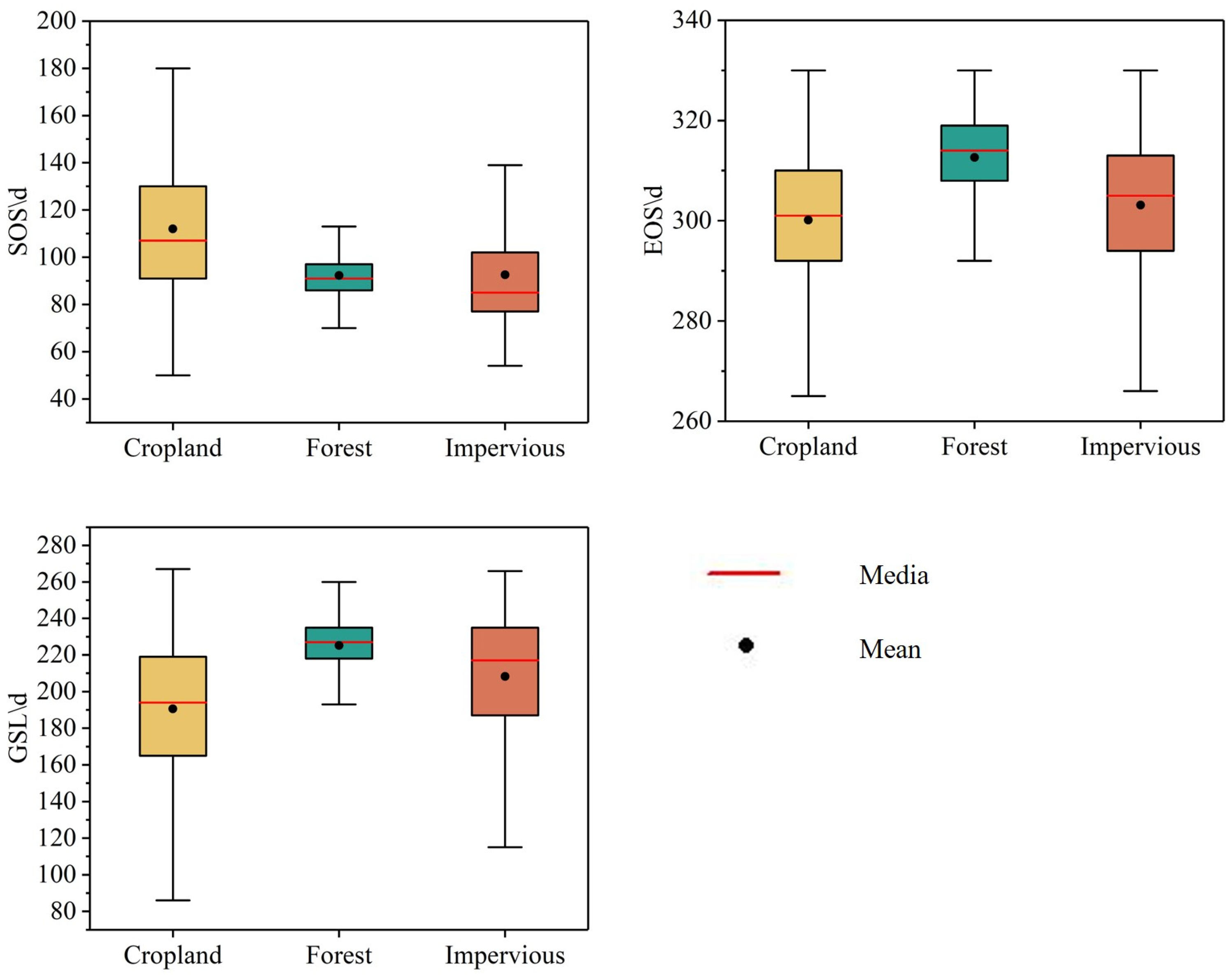
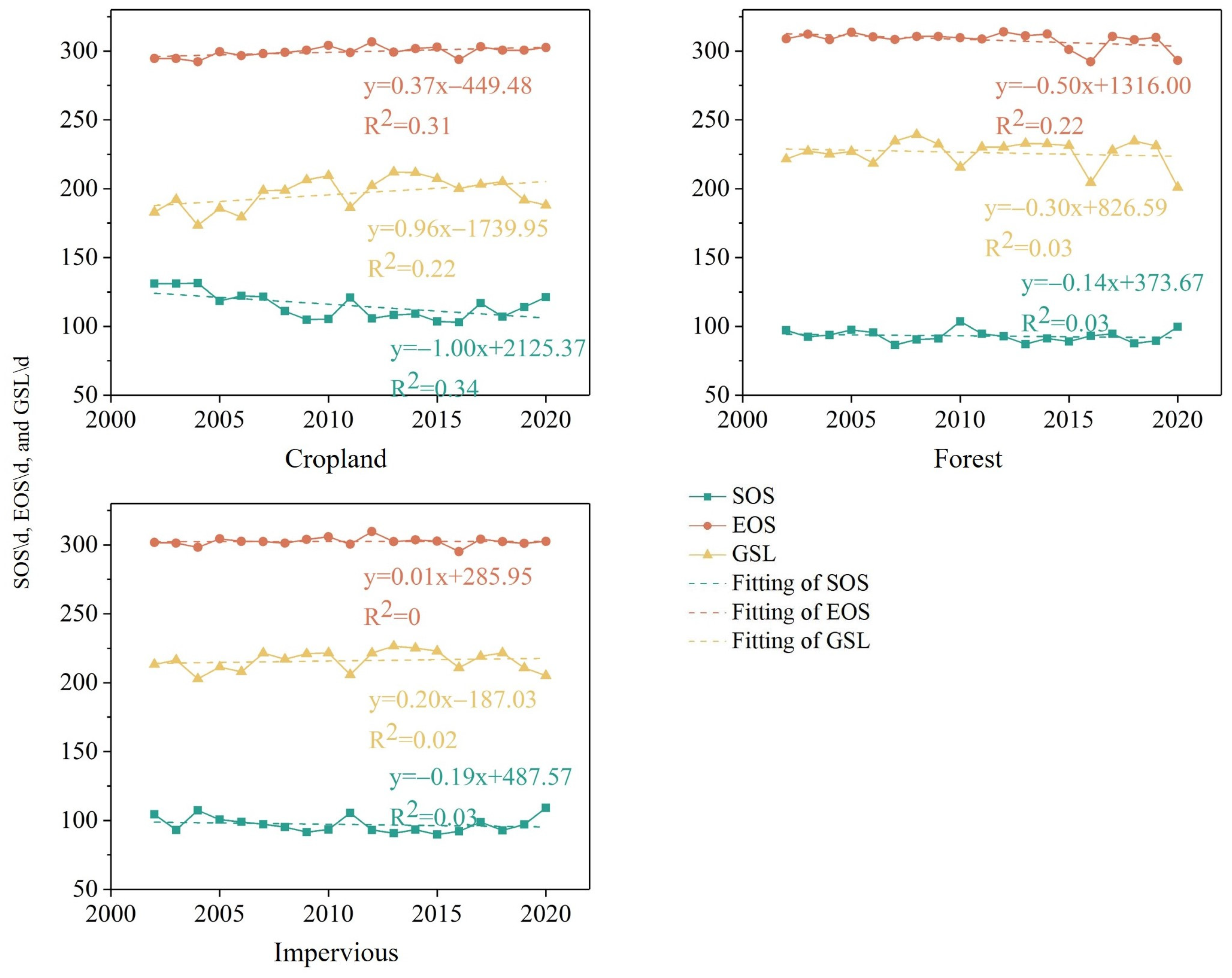
3.1.2. Differences in Vegetation Phenology between Land Covers

The results of the analysis of spatial and temporal patterns of vegetation phenology in the study area showed that there were some differences in vegetation phenology under different surface covers; we, therefore, analyzed the vegetation phenology under different land covers in the study area.

The results obtained from the preliminary analysis of vegetation phenology between different land covers are shown in Figure 7. There are significant differences in vegetation phenology under different land covers (the results of the analysis of variance (ANOVA) showed that p < 0.05 at the 0.05 level of significance, which indicates that there is a significant difference between the different land covers); in terms of the length of vegetation phenology indicators as well as earliness and lateness, the SOS in the study area is earlier in forests and impervious surfaces, at 92.27 and 92.56 days, respectively, and later in cropland, at 112.00 days; EOS was the latest in forests at 312.62 days and the earliest in cropland at 300.12 days; GSLs were longest in forests at 225.13 days, while GSL was the shortest in cropland at 190.61 days. In terms of the fluctuation of vegetation phenology indicators, forests vegetation phenology indicators had the least fluctuation with standard deviations in SOS, EOS, and GSL of 8.74, 8.27, and 13.90 days, respectively, and the greatest fluctuation was observed in cropland with standard deviations in SOS, EOS, and GSL of 25.17, 12.59, and 34.38 days, respectively. This may be due to differences in LST under different land covers and differences in vegetation types.

Figure 8 shows the changes in vegetation phenology under different land covers in the study area from 2002 to 2020. In terms of time, SOS under different land covers showed an overall trend of advancement, with the most pronounced trend in cropland at −1.00 days per year; EOS showed a significantly delayed trend in cropland, at 0.37 days per year, and forest EOS showed a significant advancement trend at −0.50 days per year, while EOS did not change significantly on impervious surfaces; GSL showed a lengthening trend on both cropland and impervious surfaces, which was most pronounced in agricultural areas at 0.96 days per year, and a shortening trend in forest GSL.

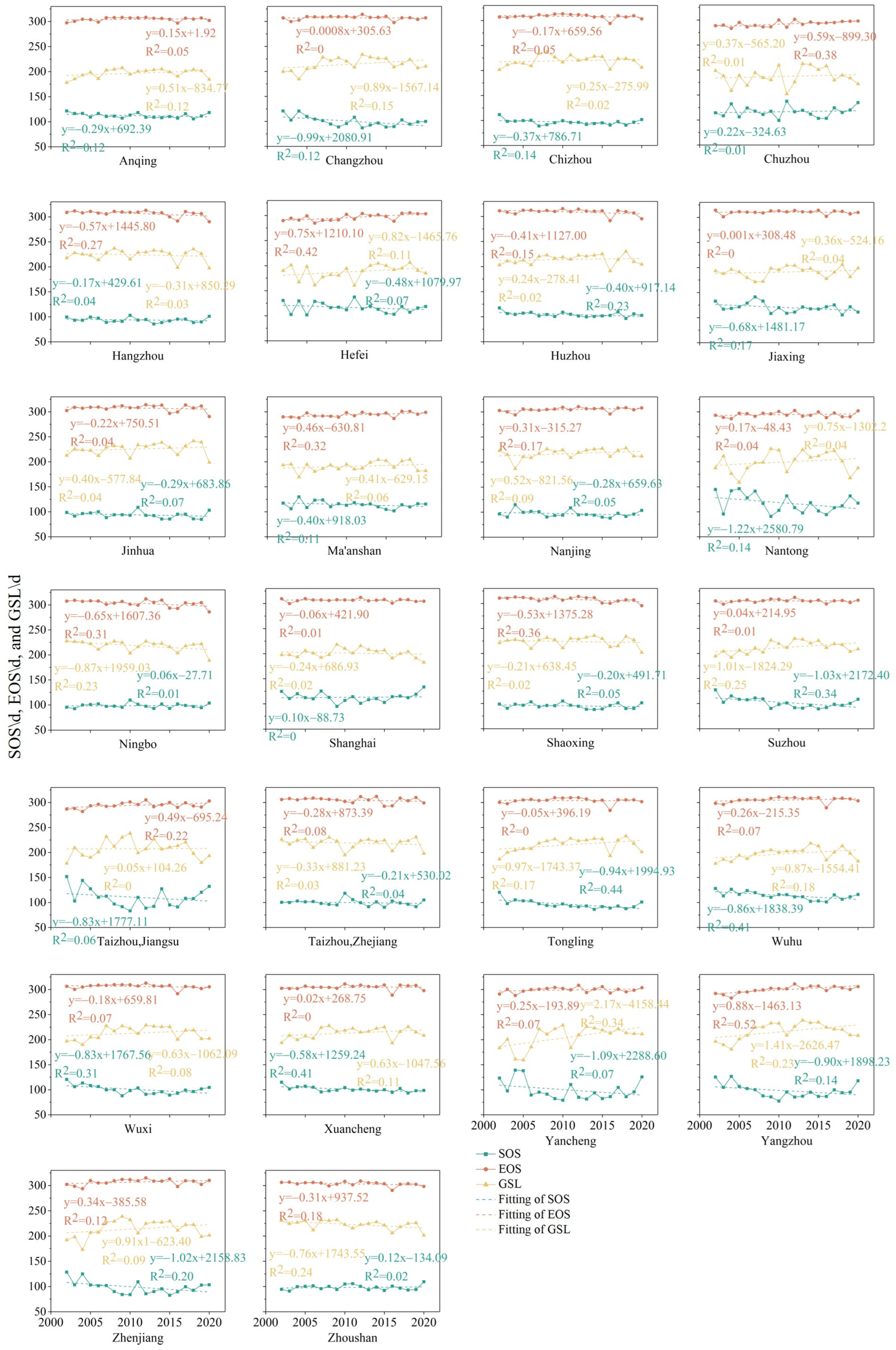
3.1.3. Differences in Vegetation Phenology by City

Figure 9 shows the vegetation phenology indicators of the cities in the study area from 2002 to 2020; it was found that in terms of spatial distribution, the SOS was earlier in several cities located in the southern part of the study area, and later in several cities located along the river in the west and east of Tai Lake. Several cities in the eastern and western parts of the river basin have earlier EOSs and cities in the south have later EOSs; several cities located in the west have shorter GSLs and several cities in the southeast and north have longer GSLs. This may be due to LST and land cover differences. In general, several cities located in the west with shorter GSLs also show a trend in later SOSs and earlier EOSs.

In terms of temporal changes, the SOS of 22 cities showed an advanced trend, and only 4 cities showed a postponed trend, and their postponed trend was insignificant (less than 0.30 days per year); this may be due to elevated LST in winter and spring. The EOS of 15 cities showed a postponed trend, and the EOS of 11 cities showed an advanced trend, of which the cities with a postponed trend in EOS were mainly located in the northern part of the study area, and the cities with the advanced trend are mainly located in the southern part of the study area; this may be related to the predominant land covers of the city, as the northern cities have more cropland while the southern cities have more forests. Finally, 20 cities showed a lengthened trend in GSL and only 6 cities showed a shortened trend in GSL, which are mainly located in the southeastern part of the study area; this may indicate that the environment in the southeastern part of the study area has gradually begun to negatively affect the growth of native vegetation.

3.2. Spatial and Temporal Patterns of LST

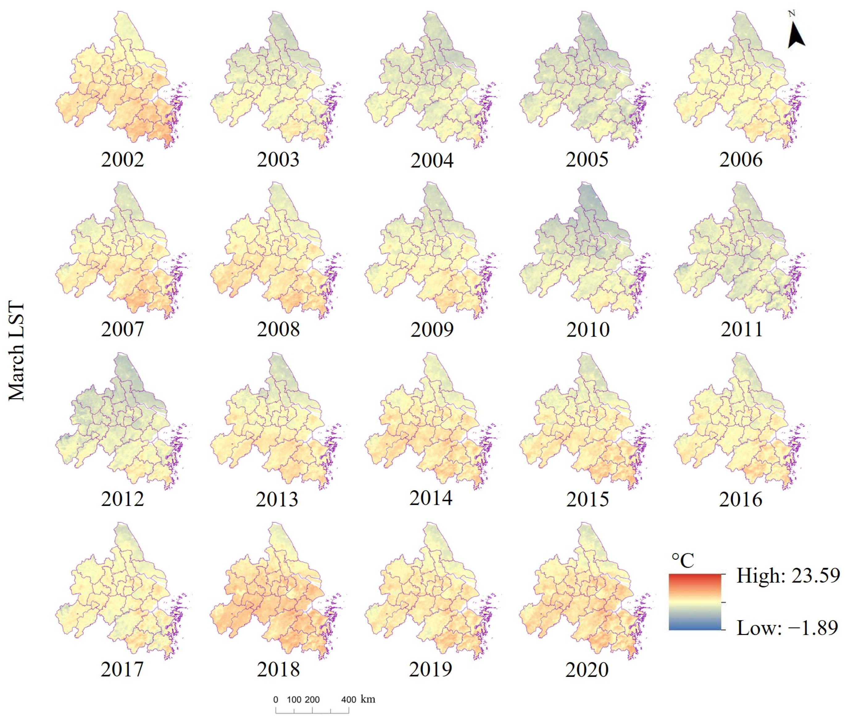
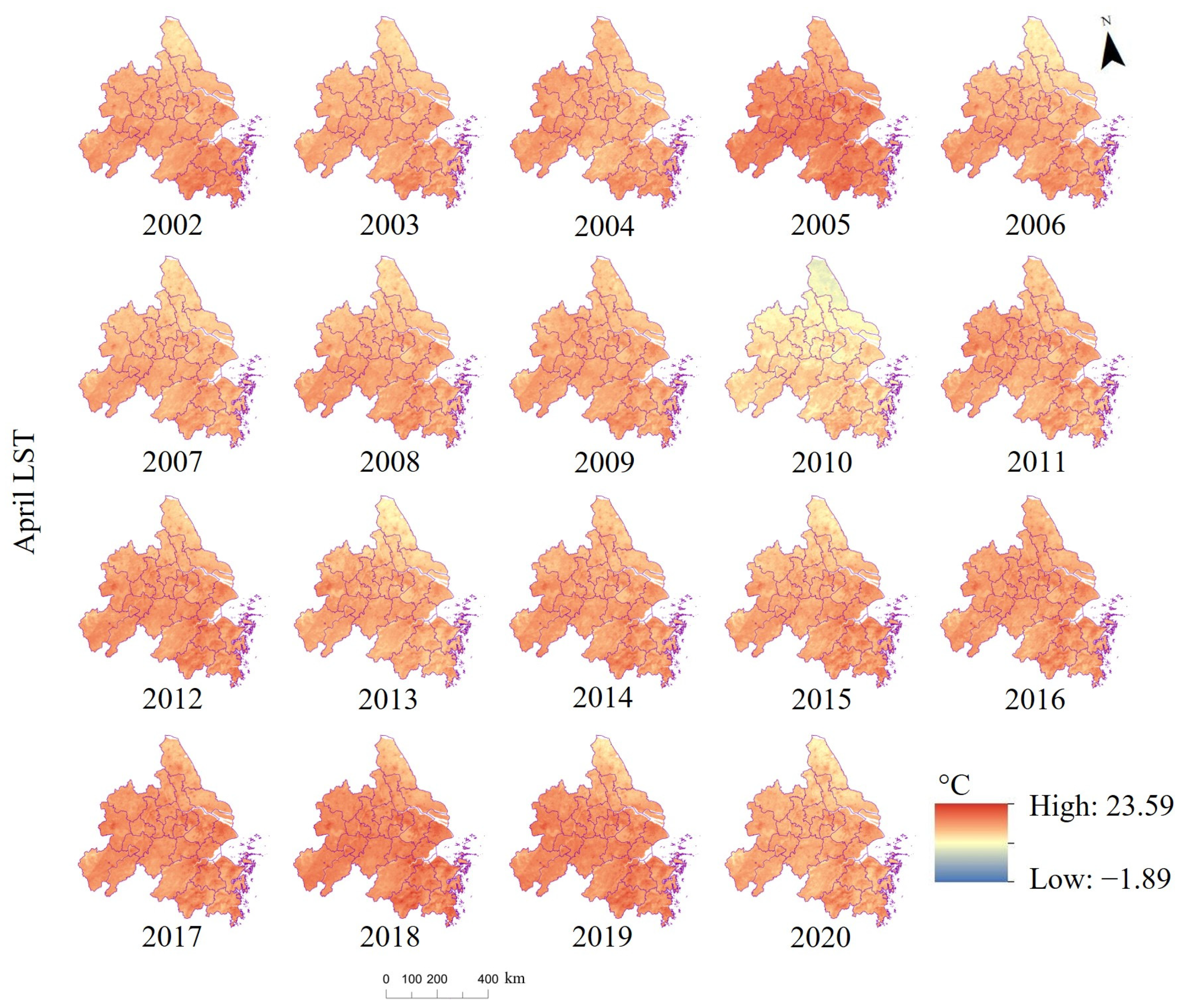
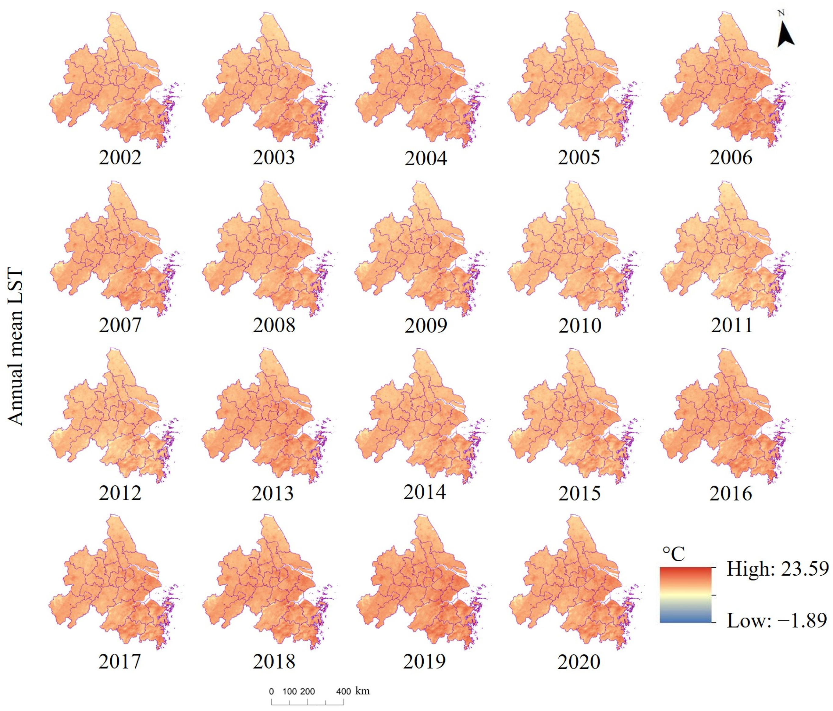
3.2.1. Spatial and Temporal Characteristics of LST in the Study Area

As shown in Figure 10, Figure 11, Figure 12 and Figure 13, the overall LST in the study area shows a gradual decrease from southeast to northwest, with the lowest LST in the north and the highest LST in the southeast, and this distribution may be related to the latitude as well as the monsoon climate of the study area. Meanwhile, the LST in the concentrated area of impervious surfaces exhibits significantly higher characteristics than the surrounding area due to the alteration in the subsurface.

Figure 14 shows the changes in LST in the study area from 2002 to 2020, and it was found that the winter LST, March LST, April LST, and annual mean LST in the study area generally showed an increased trend, with March LST showing the most pronounced increased trend, reaching 0.1 °C per year. However, LST showed a decreased trend before 2010, and an increased trend after 2010. This trend in LST was consistent with the changes in vegetation phenology, suggesting that the changes in vegetation phenology may be related to the changes in LST.

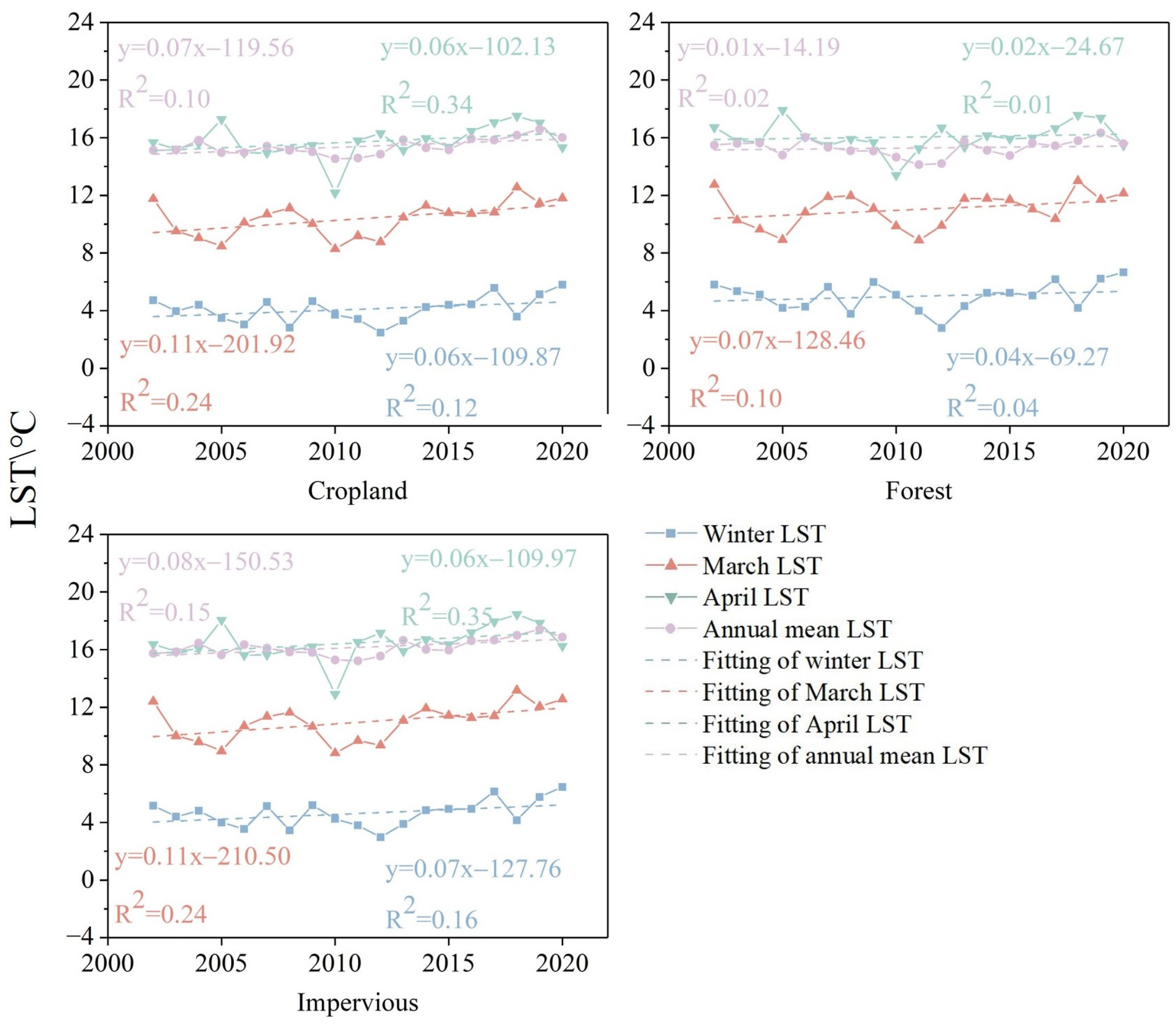
3.2.2. Differences in LST between Land Covers

Figure 15 compares differences in LST under different land covers by counting the mean annual, winter, March, and April LST from 2002 to 2020 under different land covers (the results of the ANOVA showed that p < 0.05 at the 0.05 level of significance, which indicates that there is a significant difference between the different land covers). The LST of the cropland was lowest in winter, March, and April at 4.09 °C, 10.36 °C, and 15.71 °C, respectively, with some fluctuations. Forest LST was highest in winter and March at 5.00 °C and 11.03 °C, respectively, and the annual mean LST was the lowest at 15.28 °C; it had the least fluctuating LST values, with standard deviations of 0.96 °C, 0.85 °C, 0.87 °C, and 0.92 °C for winter, March, April, and annual mean LST, respectively. Impervious surface LST was highest in April and the annual mean at 16.47 °C and 16.15 °C, respectively, which had the greatest fluctuation in LST, with the standard deviations in the annual mean, winter, March, and April LST reaching 1.46 °C, 1.37 °C, 1.52 °C, and 1.32 °C, respectively. It is possible that the special subsurface of impervious surfaces, which elevates LST more significantly than forests and agricultural fields as solar radiation is enhanced, led to the highest April and annual average LSTs on impervious surfaces.

Figure 16 shows the interannual trend in LST under different land covers, which showed an increased trend under different land covers, similar to the results for the whole study area, with the most pronounced increased trend in LST in March under the three land covers. In terms of different land covers, impervious surface LST increased at the fastest rate, with winter, March, April, and annual mean LST increasing at 0.07 °C per year, 0.11 °C per year, 0.06 °C per year, and 0.08 °C per year, respectively, while forest LST increased at the slowest rate, with winter, March, April, and annual mean LST increasing at only 0.04 °C per year, 0.07 °C per year, 0.02 °C per year, and 0.01 °C per year. It is possible that differences in the rate of increase in LST between forests and impervious surfaces were due to differences in their subsurface.

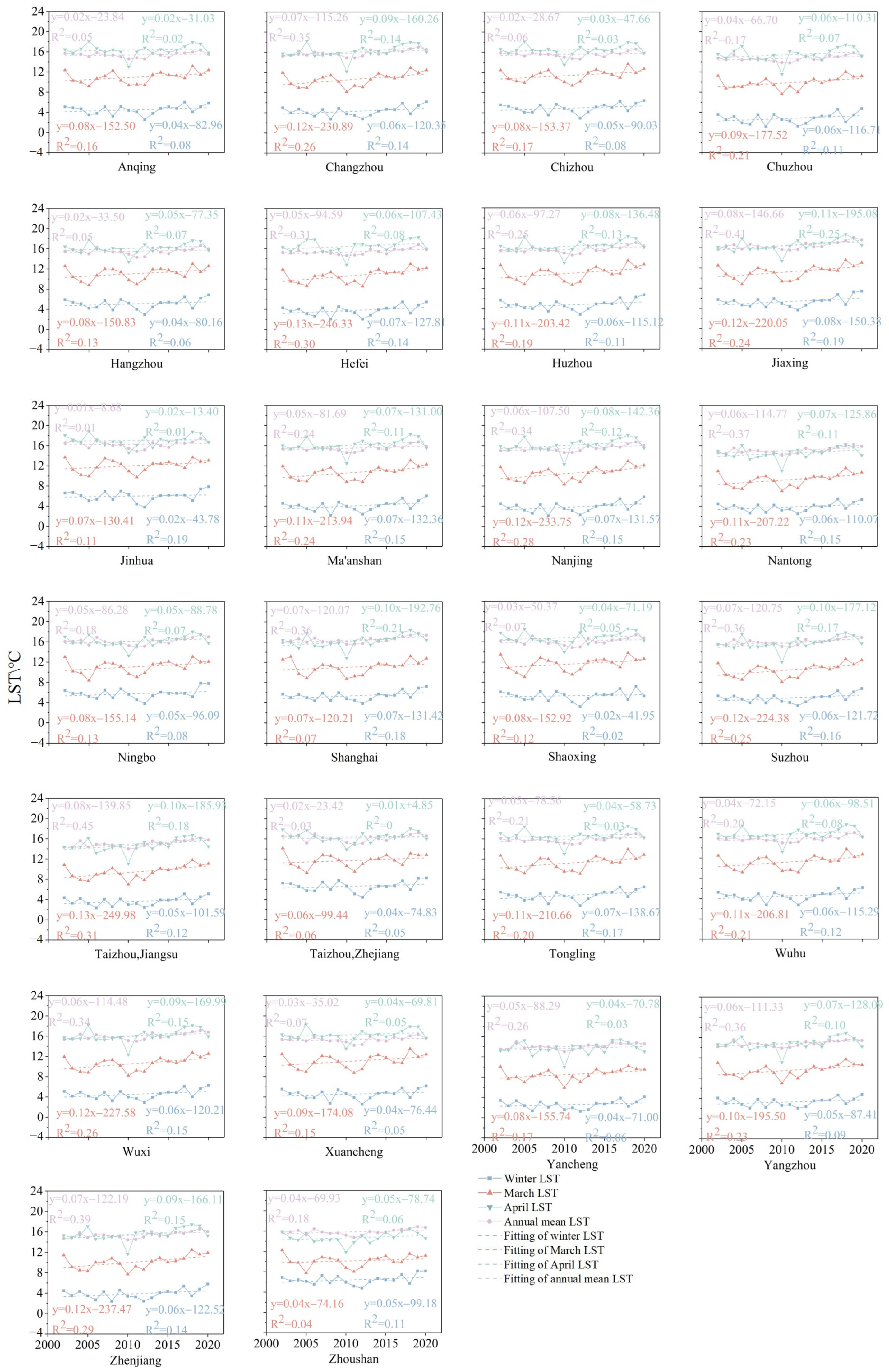
3.2.3. Differences in LST by City

Figure 17 shows the summary statistics for the LST status of each city in the study area from 2002 to 2020. In terms of spatial distribution, the cities with lower LST are mainly located in the northern part of the study area, and the cities with higher LST are mainly located in the eastern part of the study area, similar to the distribution of LST in the study area, which may be related to the latitude of the city and its exposure to the monsoon climate. What is interesting in this data is that Nantong, which is also located in the eastern part of the study area, is the northernmost city adjacent to Shanghai, but Nantong has a lower LST and Shanghai has a higher LST, which may be related to the fact that Shanghai has more impervious surfaces and strong human activities as a result of its higher urbanization intensity.

In terms of temporal changes, LST showed an increased trend in all cities from 2002 to 2020, and the cities with a more pronounced LST increased trend were mainly located in the central part of the study area, while the cities in the southern part of the study area had a slower LST increased trend; this general upward trend in LST may be due to a combination of global warming and urbanization in the study area. The variation in LST in different periods was similar to that of the whole study area, with a more pronounced trend in elevated LST in March than in winter, April, and the annual mean LST.

3.3. Response of Vegetation Phenology to LST

Based on the spatial and temporal patterns of vegetation phenology and LST in the study area, we determined that there may be a certain correlation between changes in vegetation phenology and LST. To validate our analysis, we decided to use correlation coefficients to analyze the response of vegetation phenology to LST while considering that vegetation phenology responds to LST as well as precipitation; we calculated the partial correlation coefficients between vegetation phenology and LST after excluding the precipitation factor.

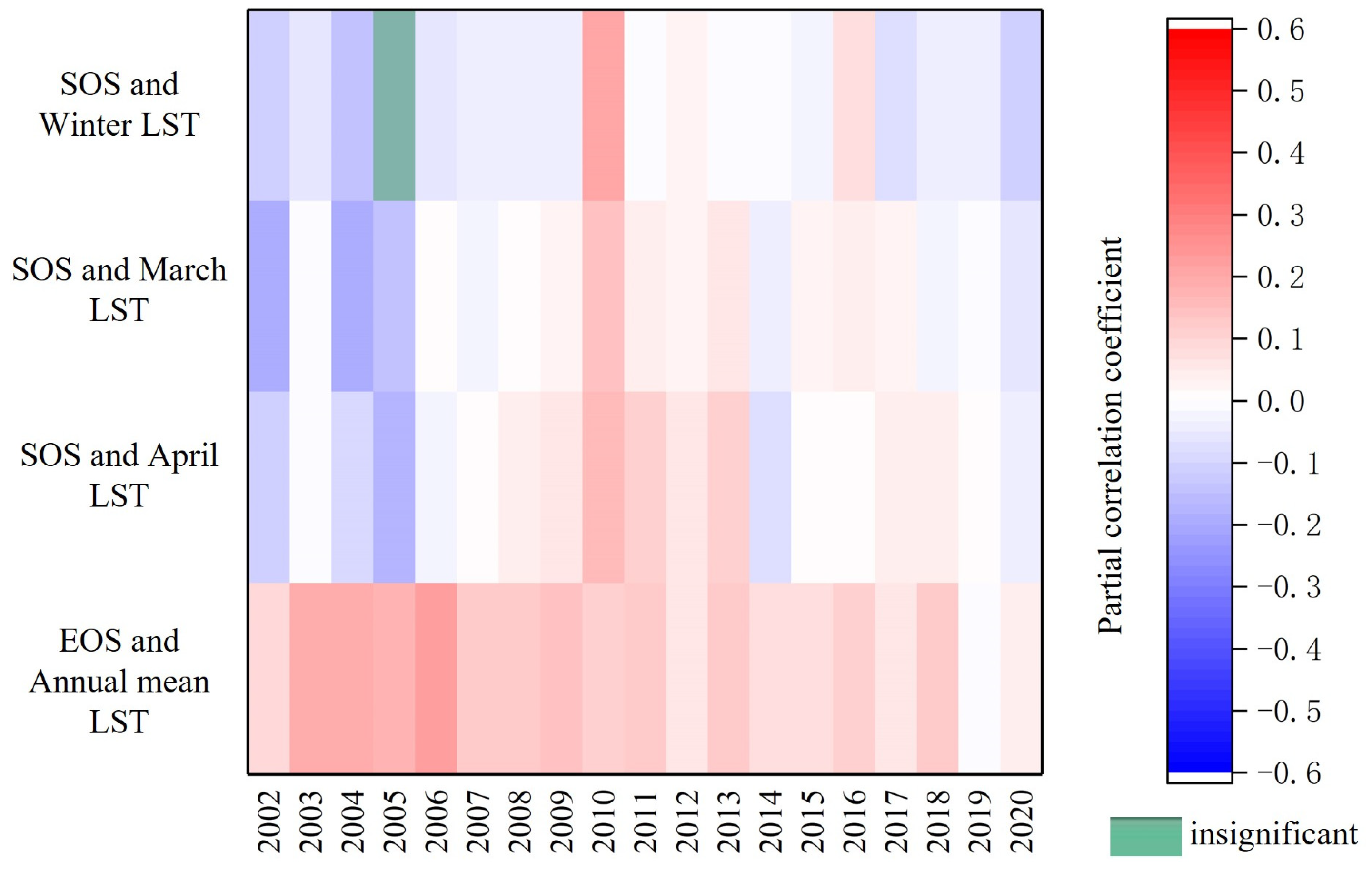
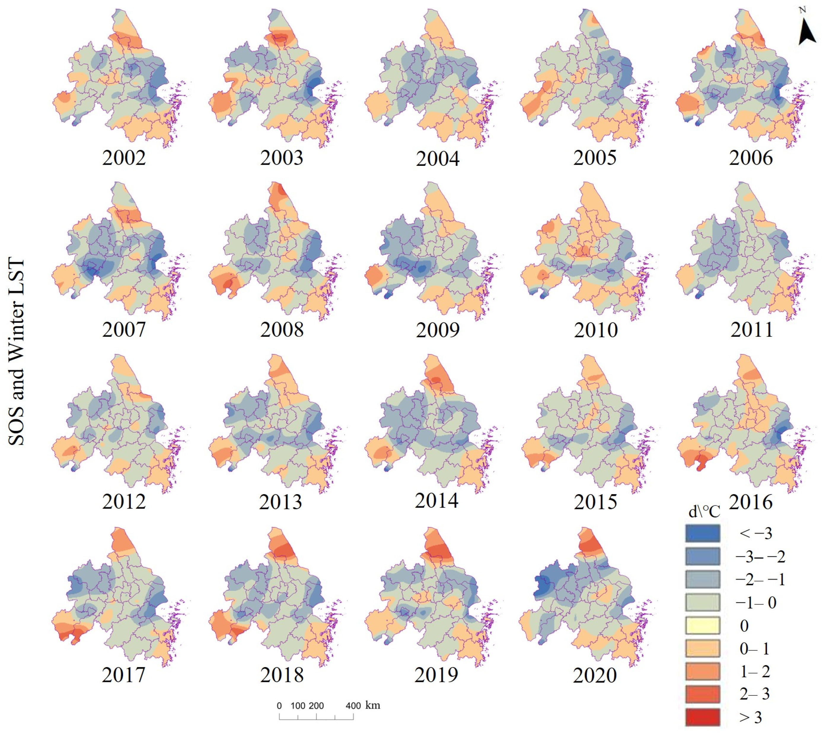
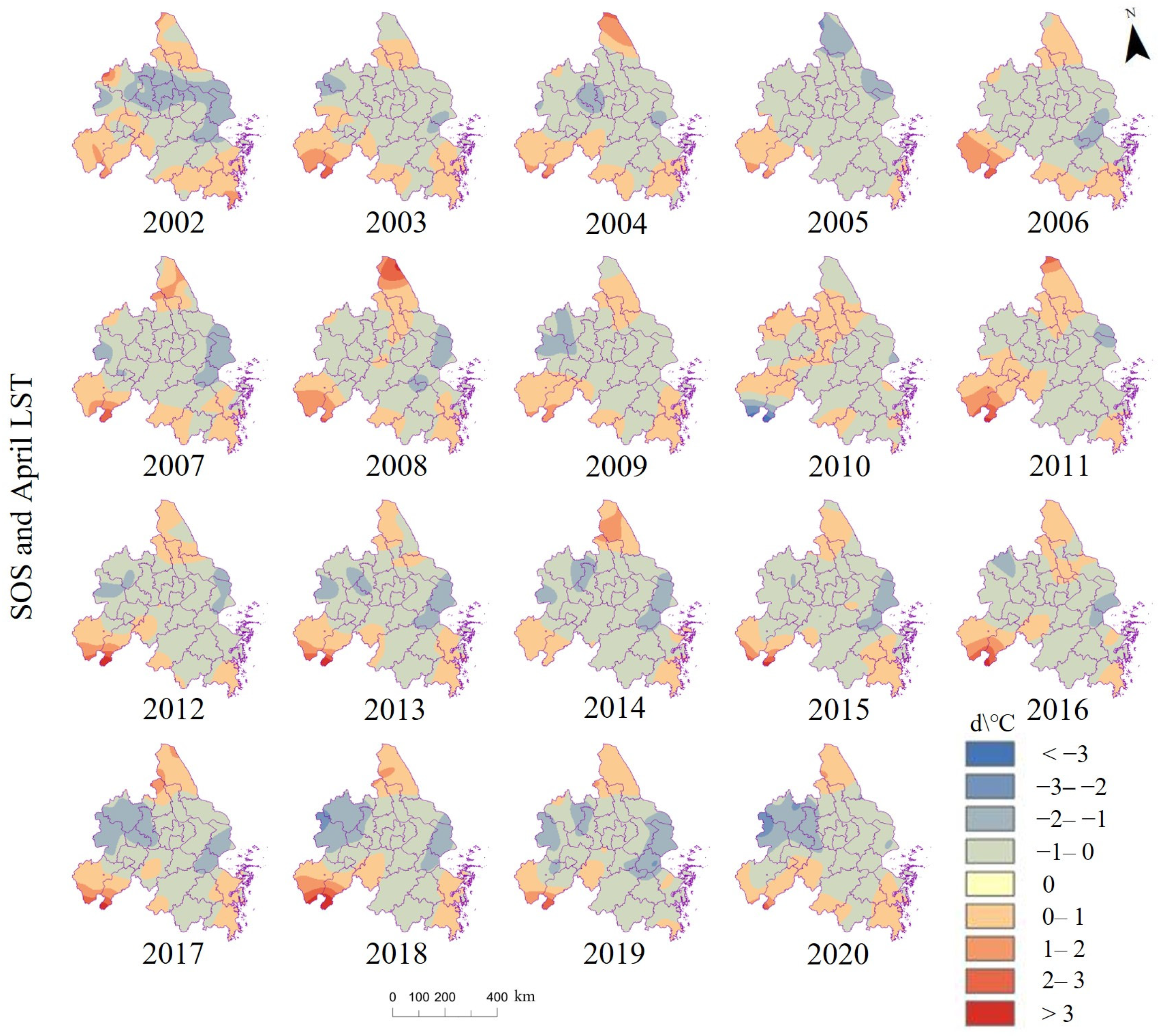
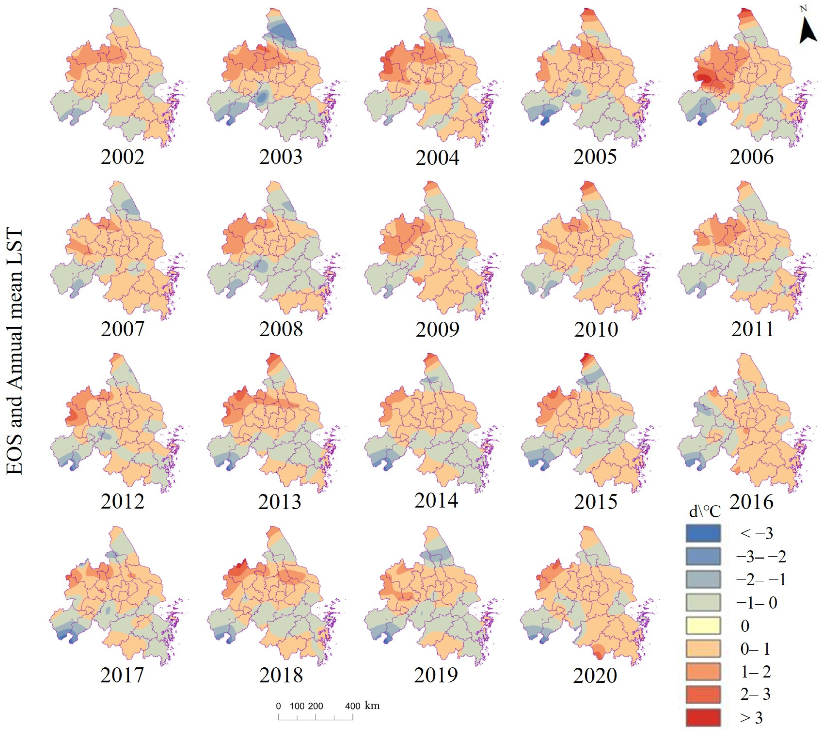
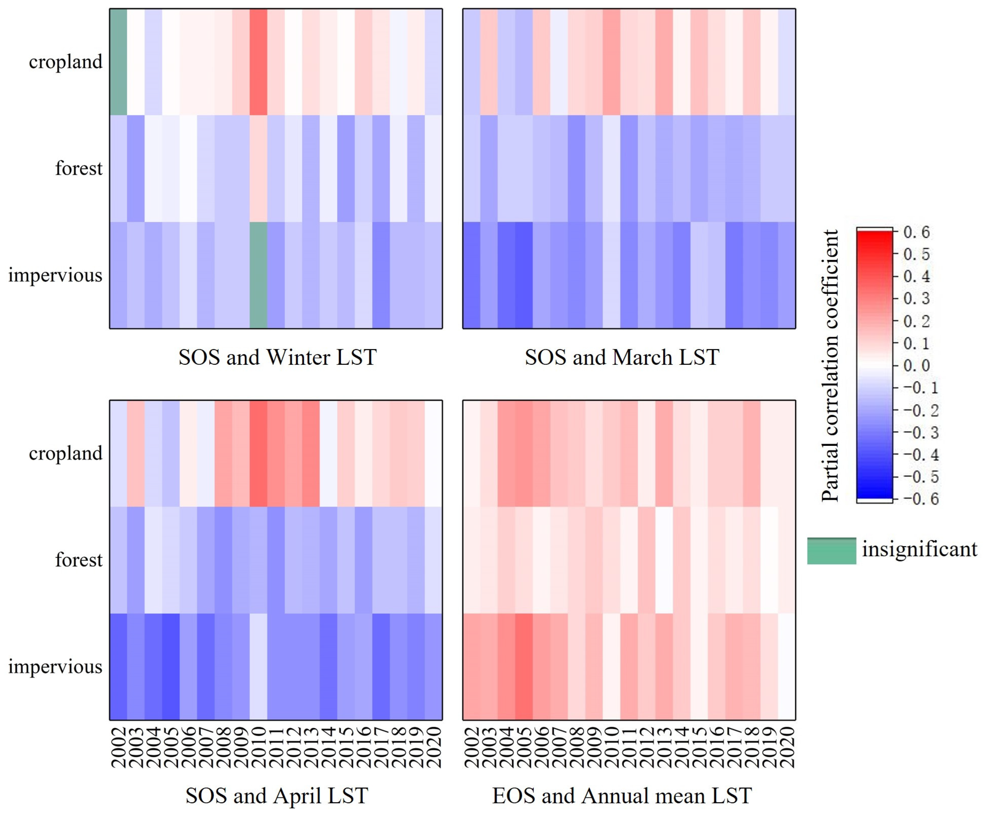
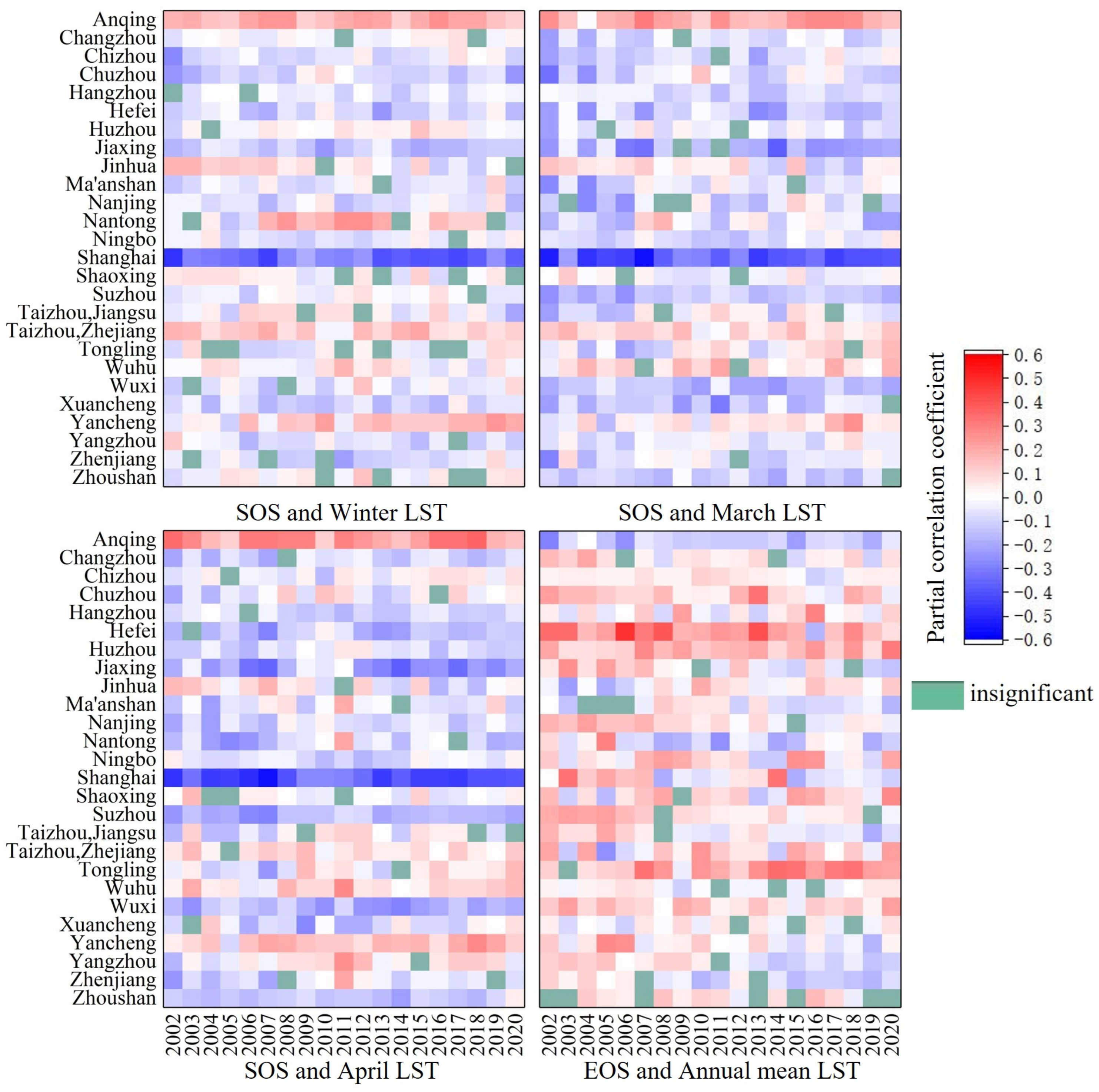
3.3.1. Partial Correlation Analysis between Vegetation Phenology and LST

Figure 18 shows the partial correlation between vegetation phenology and LST from 2002 to 2020. The partial correlation coefficients between SOS and LST in the study area showed a numerical trend of increasing and then decreasing, with the negative partial correlation gradually changing to a positive partial correlation from 2002, reaching the maximum value in 2010, and then changing to a negative partial correlation in 2020. This suggests that SOS is delayed with increasing LST around 2010, while SOS is advanced with increasing LST around 2002 and 2020. The overall partial correlation is very weak, and the absolute values of the partial coefficients between SOS and winter, March, and April LSTs are more than 0.1 in only 5, 4, and 4 years, respectively, among the 19 years. This suggests that the change in vegetation phenology with elevated LST is not very strong and that there may be a response to changes in other factors as well. From the perspective of different periods, SOS showed the most years of negatively partial correlation with winter LST and the least years of negatively partial correlation with April LST. EOS and annual LST in the study area mainly showed a significant positive partial correlation; only 2019 showed a very weak negative partial correlation, and the strength of its partial correlation was higher than that of SOS and LST, with partial correlation coefficients exceeding 0.1 in 12 years. This suggests that EOS exhibits a delayed trend with a higher average annual LST.

Figure 19, Figure 20, Figure 21 and Figure 22 show the geographically weighted regression results in the study area from 2002 to 2020. There were more areas with negative regression coefficients of SOS and LST in the study area, in which the areas with smaller regression coefficients were mainly located in the northwestern part of the study area and the eastern part of Tai Lake, and those with positive regression coefficients were mainly located in the northern, southwestern, and southeastern parts of the study area. There were more areas with positive regression coefficients of the overall EOS and the annual average LST in the study area, and the regression coefficients were the largest in the northwestern part of the study area versus those located in the southwestern and central south side of the study area.

3.3.2. Partial Correlation Analysis between Vegetation Phenology and LST for Different Land Covers

Figure 23 shows the partial correlation coefficients between vegetation phenology and LST from 2002 to 2020 for different land covers in the study area. In terms of the direction of the partial correlation coefficients, forest and impervious surface SOSs showed a significant negative partial correlation with LST, while cropland SOS mainly showed a significant positive partial correlation with LST. This suggests that forest and impervious surface SOSs exhibit an advancing trend with increasing LST, while cropland fields exhibit a delaying trend. This may be a result of differences in vegetation types under different land covers. EOS under different land covers showed a significant positive partial correlation with the average LST throughout the year. This suggests that EOS exhibits a postponement trend with increasing LST. In terms of the strength of the partial correlation, the partial correlation between vegetation phenology and LST was strongest on impervious surfaces and weakest on cropland and forest. This indicates that impervious surface vegetation phenology responds more strongly to changes in LST than forests and cropland.

Cropland SOS was most strongly and partially correlated with April LST at different times of the year; forest and impervious surfaces SOSs are strongly and partially correlated with LST in March and April. In terms of interannual trends, the partial correlation coefficients between SOS and cropland LST increased and then decreased, gradually changing from a negative partial correlation in 2002 to a positive partial correlation, reaching a maximum in 2010, and then gradually changing to a negative partial correlation in 2020. The change in the coefficient of partial correlation between SOS and forest LST fluctuates, and the strength of the negative partial correlation between SOS and impervious surfaces LST shows a tendency to decrease and then increase. The partial correlation coefficients between EOS and LST show a tendency to increase and then decrease on impervious surfaces, reaching the highest in 2005, while they fluctuate on cropland and forests. Differences in the response of vegetation phenology to LST under different land covers may result from differences in vegetation types.

3.3.3. Partial Correlation Analysis between Vegetation Phenology and LST for Different Cities

Figure 24 shows the partial correlation coefficients between vegetation phenology and LST from 2002 to 2020 for different cities in the study area, in terms of the direction of the partial correlation coefficients; SOS and LST in the cities of the study area showed a negative partial correlation in a larger number of cities. This suggests that SOS advances with increasing LST in most cities. The cities with a strong positive correlation between SOS and LST are mainly located in the northern and western riverine areas of the study area, and the land cover there is mainly cropland while the cities with a strong negative correlation between SOS and LST are mainly located in the central and eastern parts of the study area, and most of these cities have a large number of concentrated impervious surfaces. This suggests that inter-city differences in vegetation phenology in response to LST may be related to city land cover. The EOS and annual mean LST of each city mainly show positive partial correlations. This suggests that EOS exhibits a postponement trend with increasing LST.

Analyzing the strength of the LST partial correlation between SOS and different times of the year, SOS is more strongly correlated with the April LST partial correlation. In terms of temporal changes, the partial correlation coefficients between vegetation phenology and LST varied from year to year but generally showed a tendency to weaken and then strengthen. The strongest partial correlation between vegetation phenology and LST occurred mainly around 2002, 2007, and 2017, while the weaker partial correlation was mainly around 2010. This suggests that SOS responded more strongly to changes in LST in April, and the response of vegetation phenology to LST generally showed a trend of weakening and then strengthening and was significantly stronger in some years than in others.

4. Discussion

Vegetation phenology is highly sensitive to environmental changes, especially in areas of high urbanization, and environmental changes in these and surrounding areas due to intense human activities can have a significant impact on vegetation phenology [53]. Our results also found that there was a significant trend in increasing LST in the areas of concentrated impervious surfaces and that the vegetation phenology in these areas and nearby cropland changed significantly as a result of environmental changes, but the forest vegetation phenology near the areas of concentrated impervious surfaces changed relatively insignificantly. Scholars also found that the vegetation phenology of forests and shrubs was less sensitive to the surrounding environment than that of urban and cropland areas [28]. By analyzing the distribution of vegetation phenology and LST under different land covers, it was found that the vegetation phenology and LST of forests are less volatile than those of cropland and impervious surfaces, which may be related to the regulation of heat dissipation by forests themselves [54]. There is also a strong relationship between vegetation phenology and urban land cover and LST conditions in different cities; for example, cities with more forest in the southern part of the study area and more cropland in the northern part of the study area have longer GSL, while cities with more cropland in the western part of the riverine region have significantly delayed GSL due to high LST.

The results of the correlation analysis between vegetation phenology and LST showed that there were significant differences in the response of vegetation phenology to LST under different land covers, with forest and impervious surface SOS advancing with increasing LST but cropland SOS delaying with increasing LST; especially cropland near the area of concentration of impervious surfaces, SOS showed significant delay in LST increase due to urban heat island. This may be related to the following factors: (1) the urban heat island makes autumn and winter temperatures warmer and chilling accumulate insufficient, which may lead to a delay in SOS [55,56,57]; (2) differences in vegetation types, with annual herbaceous plants predominating in cropland areas and woody perennials predominating in forests and impervious surfaces, may be responsible for the different responses of vegetation phenology to temperature increases under different land covers [58]. We analyzed the partial correlation coefficients of vegetation phenology with LST and LST from 2002 to 2020 and retained the data in which the results of the linear fit of both were significant at the same time and found that neither the partial correlation coefficients of SOS with LST nor the fitted curves for LST met the conditions and that the results of the partial correlation coefficients of EOS with annual mean LST and the linear fit of annual mean LST in the three cities (Hefei, Shanghai, Yancheng) and impervious surfaces in the study area were simultaneously significant. As shown in Figure 25, the temporal variation of the correlation between vegetation phenology and LST showed that EOS exhibited a significant positive correlation with LST, but the intensity was gradually decreasing, while at the same time, the annual average LST in the study area showed a gradually increasing trend. Meanwhile, previous studies have found that the temperature sensitivity of vegetation phenology varies with temperature [59,60]. Therefore, it was judged that the elevated LST may have led to a decrease in the sensitivity of the EOS to the LST.

At the same time, there are some limitations to the content of our study. Firstly, although we have analyzed the response of vegetation phenology to LST in the Yangtze River Delta urban agglomeration, the urban agglomerations, as a region with strong and concentrated human activities, should not be neglected except for the factors of temperature and precipitation, as well as the humanistic factors such as the population density and the GDP, which are also likely to be responded to by the vegetation phenology. Secondly, previous studies have found that there can be a lag in the effect of meteorological factors on vegetation phenology [61], but we did not develop this in this study. In future studies, we hope to take into account the influence of human factors to improve the accuracy of our findings.

5. Conclusions

The main goal of the current study was to determine the spatial and temporal patterns of vegetation phenology and LST as well as the partial correlation between vegetation phenology and LST in the Yangtze River Delta urban agglomeration from 2002 to 2020 to investigate the characteristics of the spatial and temporal distributions and changes in vegetation phenology and LST under different land covers and cities over a long time series, as well as the response of vegetation phenology to LST. Accordingly, we analyzed the spatial and temporal variations of vegetation phenology and LST in the Yangtze River Delta urban agglomerations from 2002 to 2020 using vegetation phenology indicators extracted from the EVI data and the LST data and calculated the partial correlation coefficients of vegetation phenology and LST. The main conclusions were as follows:

• Characteristics of spatial and temporal variation in vegetation phenology: (1) Cities located in the area of forests in the south and concentrated impervious surfaces had an earlier SOS, later EOS, and longer GSL, while those in the east and west along the river basins had a later SOS, earlier EOS, and shorter GSL. Analyzing the different land covers showed that forests had the earliest SOS, the latest EOS, and the longest GSL, along with the least volatility in phenological indicators. The cropland had the latest SOS, the earliest EOS, the shortest GSL, and the greatest volatility in vegetation phenology indicators; phenological indicators and the volatility of impervious surfaces are intermediate between forests and cropland. The reasons for these differences may be related to differences in thermal conditions, temperatures, and dominant vegetation types under different land covers. (2) The SOS of the study area from 2002 to 2020 showed a trend of advancement; the EOS showed a trend of postponement; and the GSL showed a trend of lengthening. This trend may have been caused by the gradual increase in LST in the study area.
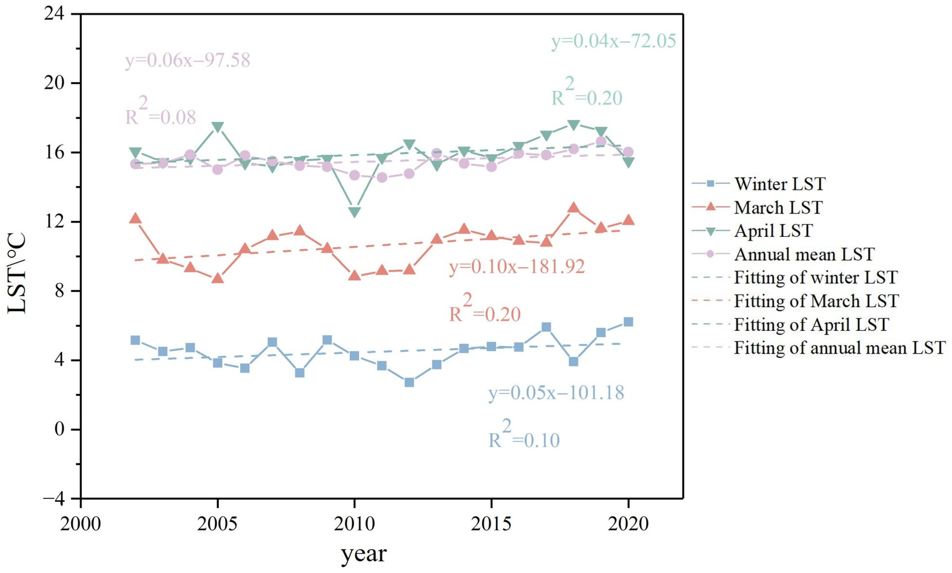
• Temporal and spatial variability characteristics of LST: (1) The LST in the study area at different times of the year generally showed a trend of gradual decrease from the southeast to the northwest. Cropland has the lowest LST in winter, March, and April; forest LST is higher in winter and March, but the annual mean LST is lower while it is the least volatile; and impervious surfaces have the highest April and annual mean LST, while they are the most volatile. This can be caused by impervious surfaces having more buildings, asphalt, and other surfaces. (2) From 2002 to 2020, winter, March, April, and annual mean LST in the study area showed an increased trend, the trend in elevated LST was most pronounced in March. This increased trend in LST may have been due to global warming and urbanization in the study area.
• Vegetation phenology response to LST: (1) Cropland SOS was delayed with increased LST while forests and impervious surfaces were advanced; this may have been caused by differences in vegetation types under different land covers, as different vegetation responds differently to changes in LST; EOS was mainly delayed as LST increased. (2) Impervious surface vegetation phenology responded most strongly to LST while cropland and forests were less responsive; this may imply that vegetation in impervious surface areas responds more significantly to changes in LST. (3) Cropland responded more strongly to April LST while forests and impervious surfaces responded more strongly to March and April; this may indicate that the SOS response to LST in March and April will be more significant than the response to LST in winter. (4) The response of vegetation phenology to LST was variable, but the years of strong response were relatively concentrated.

References

1. Xu, H.; Yang, S. Urban heat island effect and urban ecosystems. J. Beijing Norm. Univ. (Nat. Sci.) 2018, 54, 790–798. [Google Scholar] [CrossRef]
2. Liu, X.; Huang, Y.; Xu, X.; Li, X.; Li, X.; Ciais, P.; Lin, P.; Gong, K.; Ziegler, A.D.; Chen, A.; et al. High-spatiotemporal-resolution mapping of global urban change from 1985 to 2015. Nat. Sustain. 2020, 3, 564–570. [Google Scholar] [CrossRef]
3. Peng, J.; Jia, J.; Liu, Y.; Li, H.; Wu, J. Seasonal contrast of the dominant factors for spatial distribution of land surface temperature in urban areas. Remote Sens. Environ. 2018, 215, 255–267. [Google Scholar] [CrossRef]
4. Nayak, H.P.; Nandini, G.; Vinoj, V.; Landu, K.; Swain, D.; Mohanty, U.C.; Niyogi, D. Influence of urbanization on winter surface temperatures in a topographically asymmetric Tropical City, Bhubaneswar, India. Comput. Urban Sci. 2023, 3, 36. [Google Scholar] [CrossRef]
5. Kabano, P.; Lindley, S.; Harris, A. Evidence of urban heat island impacts on the vegetation growing season length in a tropical city. Landsc. Urban Plan. 2021, 206, 103989. [Google Scholar] [CrossRef]
6. Richardson, A.D.; Hollinger, D.Y.; Dail, D.B.; Lee, J.T.; Munger, J.W.; O’keefe, J. Influence of spring phenology on seasonal and annual carbon balance in two contrasting New England forests. Tree Physiol. 2009, 29, 321–331. [Google Scholar] [CrossRef]
7. Qiu, T.; Song, C.; Zhang, Y.; Liu, H.; Vose, J.M. Urbanization and climate change jointly shift land surface phenology in the northern mid-latitude large cities. Remote Sens. Environ. 2020, 236, 111477. [Google Scholar] [CrossRef]
8. Zhao, S.; Liu, S.; Zhou, D. Prevalent vegetation growth enhancement in urban environment. Proc. Natl. Acad. Sci. USA 2016, 113, 6313–6318. [Google Scholar] [CrossRef]
9. Li, X.; Zhou, Y.; Meng, L.; Asrar, G.; Sapkota, A.; Coates, F. Characterizing the relationship between satellite phenology and pollen season: A case study of birch. Remote Sens. Environ. 2019, 222, 267–274. [Google Scholar] [CrossRef]
10. Xia, C.; Li, J.; Liu, Q. Review of advances in vegetation phenology monitoring by remote sensing. Natl. Remote Sens. Bull. 2013, 17, 1–16. [Google Scholar]
11. Piao, S.; Mohammat, A.; Fang, J.; Cai, Q.; Feng, J. NDVI-based increase in growth of temperate grasslands and its responses to climate changes in China. Glob. Environ. Chang. 2006, 16, 340–348. [Google Scholar] [CrossRef]
12. Cleland, E.E.; Chuine, I.; Menzel, A.; Mooney, H.A.; Schwartz, M.D. Shifting plant phenology in response to global change. Trends Ecol. Evol. 2007, 22, 357–365. [Google Scholar] [CrossRef]
13. Jeong, S.-J.; Ho, C.-H.; Gim, H.-J.; Brown, M.E. Phenology shifts at start vs. end of growing season in temperate vegetation over the Northern Hemisphere for the period 1982–2008. Glob. Chang. Biol. 2011, 17, 2385–2399. [Google Scholar] [CrossRef]
14. Keenan, T.F.; Gray, J.; Friedl, M.A.; Toomey, M.; Bohrer, G.; Hollinger, D.Y.; Munger, J.W.; O’Keefe, J.; Schmid, H.P.; Wing, I.S. Net carbon uptake has increased through warming-induced changes in temperate forest phenology. Nat. Clim. Chang. 2014, 4, 598–604. [Google Scholar] [CrossRef]
15. Richardson, A.D.; Andy Black, T.; Ciais, P.; Delbart, N.; Friedl, M.A.; Gobron, N.; Hollinger, D.Y.; Kutsch, W.L.; Longdoz, B.; Luyssaert, S.; et al. Influence of spring and autumn phenological transitions on forest ecosystem productivity. Philos. Trans. R. Soc. Lond. Ser. B Biol. Sci. 2010, 365, 3227–3246. [Google Scholar] [CrossRef]
16. Piao, S.; Ciais, P.; Friedlingstein, P.; Peylin, P.; Reichstein, M.; Luyssaert, S.; Margolis, H.; Fang, J.; Barr, A.; Chen, A.; et al. Net carbon dioxide losses of northern ecosystems in response to autumn warming. Nature 2008, 451, 49–52. [Google Scholar] [CrossRef]
17. Zeng, H.; Jia, G.; Epstein, H. Recent changes in phenology over the northern high latitudes detected from multi-satellite data. Environ. Res. Lett. 2011, 6, 045508. [Google Scholar] [CrossRef]
18. Dragoni, D.; Rahman, A.F. Trends in fall phenology across the deciduous forests of the Eastern USA. Agric. For. Meteorol. 2012, 157, 96–105. [Google Scholar] [CrossRef]
19. Aono, Y.; Kazui, K. Phenological data series of cherry tree flowering in Kyoto, Japan, and its application to reconstruction of springtime temperatures since the 9th century. Int. J. Climatol. 2008, 28, 905–914. [Google Scholar] [CrossRef]
20. Annette, M.; Ye, Y.; Michael, M.; Tim, S.; Helfried, S.; Regula, G.; Nicole, E. Climate change fingerprints in recent European plant phenology. Glob. Chang. Biol. 2020, 26, 2599–2612. [Google Scholar] [CrossRef]
21. Jochner, S.; Menzel, A. Urban phenological studies—Past, present, future. Environ. Pollut. 2015, 203, 250–261. [Google Scholar] [CrossRef]
22. Zhang, X.; Friedl, M.A.; Schaaf, C.B.; Strahler, A.H.; Schneider, A. The footprint of urban climates on vegetation phenology. Geophys. Res. Lett. 2004, 31, L122091–L122094. [Google Scholar] [CrossRef]
23. Zhou, D.; Zhao, S.; Zhang, L.; Liu, S. Remotely sensed assessment of urbanization effects on vegetation phenology in China’s 32 major cities. Remote Sens. Environ. 2016, 176, 272–281. [Google Scholar] [CrossRef]
24. Ji, Y.; Zhan, W.; Du, H.; Wang, S.; Li, L.; Xiao, J.; Liu, Z.; Huang, F.; Jin, J. Urban-rural gradient in vegetation phenology changes of over 1500 cities across China jointly regulated by urbanization and climate change. ISPRS J. Photogramm. Remote Sens. 2023, 205, 367–384. [Google Scholar] [CrossRef]
25. Zhu, E.; Fang, D.; Chen, L.; Qu, Y.; Liu, T. The Impact of Urbanization on Spatial–Temporal Variation in Vegetation Phenology: A Case Study of the Yangtze River Delta, China. Remote Sens. 2024, 16, 914. [Google Scholar] [CrossRef]
26. Jia, W.; Zhao, S.; Zhang, X.; Liu, S.; Henebry, G.M.; Liu, L. Urbanization imprint on land surface phenology: The urban–rural gradient analysis for Chinese cities. Glob. Chang. Biol. 2021, 27, 2895–2904. [Google Scholar] [CrossRef]
27. Yang, J.; Luo, X.; Jin, C.; Xiao, X.; Xia, J. Spatiotemporal patterns of vegetation phenology along the urban–rural gradient in Coastal Dalian, China. Urban For. Urban Green. 2020, 54, 126784. [Google Scholar] [CrossRef]
28. Zhang, Y.; Yin, P.; Li, X.; Niu, Q.; Wang, Y.; Cao, W.; Huang, J.; Chen, H.; Yao, X.; Yu, L.; et al. The divergent response of vegetation phenology to urbanization: A case study of Beijing city, China. Sci. Total Env. 2022, 803, 150079. [Google Scholar] [CrossRef]
29. Zhou, D.; Zhao, S.; Zhang, L.; Sun, G.; Liu, Y. The footprint of urban heat island effect in China. Sci. Rep. 2015, 5, 11160. [Google Scholar] [CrossRef]
30. Wang, M.; Luo, Y.; Zhang, Z.; Xie, Q.; Wu, X.; Ma, X. Recent advances in remote sensing of vegetation phenology: Retrieval algorithm and validation strategy. Natl. Remote Sens. Bull. 2022, 26, 431–455. [Google Scholar] [CrossRef]
31. Justice, C.O.; Vermote, E.; Townshend, J.R.; Defries, R.; Roy, D.P.; Hall, D.K.; Salomonson, V.V.; Privette, J.L.; Riggs, G.; Strahler, A.; et al. Moderate Resolution Imaging Spectroradiometer (MODIS): Land remote sensing for global change research. IEEE Trans. Geosci. Remote Sens. 1998, 36, 1228–1249. [Google Scholar] [CrossRef]
32. Rizvi, S.H.; Fatima, H.; Iqbal, M.J.; Alam, K. The effect of urbanization on the intensification of SUHIs: Analysis by LULC on Karachi. J. Atmos. Sol. Terr. Phys. 2020, 207, 105374. [Google Scholar] [CrossRef]
33. Siddiqui, A.; Kushwaha, G.; Nikam, B.; Srivastav, S.K.; Shelar, A.; Kumar, P. Analysing the day/night seasonal and annual changes and trends in land surface temperature and surface urban heat island intensity (SUHII) for Indian cities. Sustain. Cities Soc. 2021, 75, 103374. [Google Scholar] [CrossRef]
34. Yin, P.; Li, X.; Zhou, Y.; Mao, J.; Fu, Y.H.; Cao, W.; Gong, P.; He, W.; Li, B.; Huang, J.; et al. Urbanization effects on the spatial patterns of spring vegetation phenology depend on the climatic background. Agric. For. Meteorol. 2024, 345, 109718. [Google Scholar] [CrossRef]
35. Tang, W.; Zhou, J.; Ma, J.; Wang, Z.; Ding, L.; Zhang, X.; Zhang, X. TRIMS LST: A daily 1-km all-weather land surface temperature dataset for the Chinese landmass and surrounding areas (2000–2021). Earth Syst. Sci. Data Discuss. 2023, 2023, 1–34. [Google Scholar] [CrossRef]
36. Zhou, J.; Zhang, X.; Zhan, W.; Gottsche, F.M.; Liu, S.; Olesen, F.S.; Hu, W.; Dai, F. A Thermal Sampling Depth Correction Method for Land Surface Temperature Estimation From Satellite Passive Microwave Observation Over Barren Land. IEEE Trans. Geosci. Remote Sens. 2017, 55, 4743–4756. [Google Scholar] [CrossRef]
37. Zhang, X.; Zhou, J.; Göttsche, F.-M.; Zhan, W.; Liu, S.; Cao, R. A Method Based on Temporal Component Decomposition for Estimating 1-km All-Weather Land Surface Temperature by Merging Satellite Thermal Infrared and Passive Microwave Observations. IEEE Trans. Geosci. Remote Sens. A Publ. IEEE Geosci. Remote Sens. Soc. 2019, 57, 4670–4691. [Google Scholar] [CrossRef]
38. Zhang, X.; Zhou, J.; Liang, S.; Wang, D. A practical reanalysis data and thermal infrared remote sensing data merging (RTM) method for reconstruction of a 1-km all-weather land surface temperature. Remote Sens. Environ. 2021, 260, 112437. [Google Scholar] [CrossRef]
39. Ji, Y.; Jin, J.; Zhan, W.; Guo, F.; Yan, T. Quantification of Urban Heat Island-Induced Contribution to Advance in Spring Phenology: A Case Study in Hangzhou, China. Remote Sens. 2021, 13, 3684. [Google Scholar] [CrossRef]
40. Polgar, C.; Gallinat, A.; Primack, R.B. Drivers of leaf-out phenology and their implications for species invasions: Insights from Thoreau’s Concord. New Phytol. 2014, 202, 106–115. [Google Scholar] [CrossRef]
41. Gou, J.; Miao, C.; Samaniego, L.; Xiao, M.; Wu, J.; Guo, X. CNRD v1.0: A High-Quality Natural Runoff Dataset for Hydrological and Climate Studies in China. Bull. Am. Meteorol. Soc. 2021, 102, E929–E947. [Google Scholar] [CrossRef]
42. Miao, C.; Gou, J.; Fu, B.; Tang, Q.; Duan, Q.; Chen, Z.; Lei, H.; Chen, J.; Guo, J.; Borthwick, A.G.L.; et al. High-quality reconstruction of China’s natural streamflow. Sci. Bull. 2022, 67, 547–556. [Google Scholar] [CrossRef]
43. Han, J.Y.; Miao, C.Y.; Gou, J.J.; Zheng, H.Y.; Zhang, Q.; Guo, X.Y. A new daily gridded precipitation dataset for the Chinese mainland based on gauge observations. Earth Syst. Sci. Data 2023, 15, 3147–3161. [Google Scholar] [CrossRef]
44. Yang, J.; Huang, X. The 30 m annual land cover datasets and its dynamics in China from 1985 to 2022. Earth Syst. Sci. Data 2021, 13, 3907–3925. [Google Scholar] [CrossRef]
45. Chen, J.; Jönsson, P.; Tamura, M.; Gu, Z.; Matsushita, B.; Eklundh, L. A simple method for reconstructing a high-quality NDVI time-series data set based on the Savitzky–Golay filter. Remote Sens. Environ. 2004, 91, 332–344. [Google Scholar] [CrossRef]
46. Jönsson, P.; Eklundh, L. Seasonality extraction by function fitting to time-series of satellite sensor data. IEEE Trans. Geosci. Remote Sens. 2002, 40, 1824–1832. [Google Scholar] [CrossRef]
47. Beck, P.S.A.; Atzberger, C.; Høgda, K.A.; Johansen, B.; Skidmore, A.K. Improved monitoring of vegetation dynamics at very high latitudes: A new method using MODIS NDVI. Remote Sens. Environ. 2006, 100, 321–334. [Google Scholar] [CrossRef]
48. Song, C.; Linggong, K.E.; Liu, S.; Liu, G.; Zhong, X. Comparison of Three NDVI Timeseries Fitting Methods based on TIMESAT—Taking the Grassland in Northern Tibet as Case. Remote Sens. Technol. Appl. 2011, 26, 147–155. [Google Scholar] [CrossRef]
49. Liang, L.; Schwartz, M.D.; Fei, S. Validating satellite phenology through intensive ground observation and landscape scaling in a mixed seasonal forest. Remote Sens. Environ. 2011, 115, 143–157. [Google Scholar] [CrossRef]
50. Ganguly, S.; Friedl, M.A.; Tan, B.; Zhang, X.; Verma, M. Land surface phenology from MODIS: Characterization of the Collection 5 global land cover dynamics product. Remote Sens. Environ. 2010, 114, 1805–1816. [Google Scholar] [CrossRef]
51. He, Y.; Fan, G.; Zhang, X.; Li, Z.; Gao, D. Vegetation Phenological Variation and Its Response to Climate Changes in Zhejiang Province. J. Nat. Resour. 2013, 28, 220–233. [Google Scholar] [CrossRef]
52. Song, C.; You, S.; Ke, L.; Liu, G.; Zhong, X. Phenological variation of typical vegetation types in northern Tibet and its response to climate changes. Acta Ecol. Sin. 2012, 32, 1045–1055. [Google Scholar] [CrossRef]
53. Yuan, H.; Yan, J.; Zang, J.; Wang, Z.; Xu, W.; Zhang, H. Influences of climate change and human activities on vegetation phenology of Shanghai. Acta Ecol. Sin. 2023, 43, 8803–8815. [Google Scholar] [CrossRef]
54. Yosef, R.; Rakholia, S.; Mehta, A.; Bhatt, A.; Kumbhojkar, S. Land Surface Temperature Regulation Ecosystem Service: A Case Study of Jaipur, India, and the Urban Island of Jhalana Reserve Forest. Forests 2022, 13, 1101. [Google Scholar] [CrossRef]
55. Heide, O.M. High autumn temperature delays spring bud burst in boreal trees, counterbalancing the effect of climatic warming. Tree Physiol. 2003, 23, 931–936. [Google Scholar] [CrossRef]
56. Chuine, I.; Morin, X.; Bugmann, H. Warming, photoperiods, and tree phenology. Science 2010, 329, 277–278. [Google Scholar] [CrossRef]
57. Chung, U.; Jung, J.-e.; Seo, H.-c.; Yun, J.I. Using urban effect corrected temperature data and a tree phenology model to project geographical shift of cherry flowering date in South Korea. Clim. Chang. 2009, 93, 447–463. [Google Scholar] [CrossRef]
58. Lai, X.; Li, M.; Liu, C.; Zhong, Y.; Lin, L.; Wang, H. The phenological responses of plants to the heat island effect in the main urban area of Chongqing. Acta Ecol. Sin. 2019, 39, 7025–7034. [Google Scholar] [CrossRef]
59. Gusewell, S.; Furrer, R.; Gehrig, R.; Pietragalla, B. Changes in temperature sensitivity of spring phenology with recent climate warming in Switzerland are related to shifts of the preseason. Glob. Chang. Biol. 2017, 23, 5189–5202. [Google Scholar] [CrossRef]
60. Wang, L.; De Boeck, H.J.; Chen, L.; Song, C.; Chen, Z.; McNulty, S.; Zhang, Z. Urban warming increases the temperature sensitivity of spring vegetation phenology at 292 cities across China. Sci. Total Environ. 2022, 834, 155154. [Google Scholar] [CrossRef]
61. Deng, C.; Bai, H.; Gao, S.; Huang, X.; Meng, Q.; Zhao, T.; Zhang, Y.; Su, K.; Guo, S. Comprehensive effect of climatic factors on plant phenology in Qinling Mountains region during 1964–2015. Acta Ecol. Sin. 2018, 73, 917–931. [Google Scholar] [CrossRef]
Figure 1. Land cover conditions in the Yangtze River Delta urban agglomeration in 2002–2020. “Land covers change” for areas where there has been a change in land covers from 2002 to 2020. Others for no change in land cover from 2002 to 2020.
Forests 15 01363 g001
Figure 2. Research framework and workflow of this study. EVI: enhanced vegetation index. LST: land surface temperature. A-G: the fits to asymmetric Gaussians.
Forests 15 01363 g002
Figure 3. Spatial and temporal deviations in SOS in the Yangtze River Delta urban agglomeration in 2002–2020. SOS: the start of the growing season.
Forests 15 01363 g003
Figure 4. Spatial and temporal deviations in EOS in the Yangtze River Delta urban agglomeration in 2002–2020. EOS: the end of the growing season.
Forests 15 01363 g004
Figure 5. Spatial and temporal deviations in GSL in the Yangtze River Delta urban agglomeration in 2002–2020. GSL: the growing season length.
Forests 15 01363 g005
Figure 6. Time series of vegetation phenology in the Yangtze River Delta urban agglomeration in 2002–2020.
Forests 15 01363 g006
Figure 7. Differences in vegetation phenology under different land covers in the Yangtze River Delta urban agglomeration (2002–2020 average).
Forests 15 01363 g007
Figure 8. Time series of vegetation phenology for different land covers in the Yangtze River Delta urban agglomerations in 2002–2020.
Forests 15 01363 g008
Figure 9. Time series of vegetation phenology in different cities of the Yangtze River Delta urban agglomeration in 2002–2020.
Forests 15 01363 g009
Figure 10. Spatial and temporal deviations in winter LST in the Yangtze River Delta urban agglomeration in 2002–2020.
Forests 15 01363 g010
Figure 11. Spatial and temporal deviations in March LST in the Yangtze River Delta urban agglomeration in 2002–2020.
Forests 15 01363 g011
Figure 12. Spatial and temporal deviations in April LST in the Yangtze River Delta urban agglomeration in 2002–2020.
Forests 15 01363 g012
Figure 13. Spatial and temporal deviations in annual mean LST in the Yangtze River Delta urban agglomeration in 2002–2020.
Forests 15 01363 g013
Figure 14. Time series of LST in the Yangtze River Delta urban agglomeration in 2002–2020.
Forests 15 01363 g014
Figure 15. Differences in LST under different land covers in the Yangtze River Delta urban agglomeration (2002–2020 average).
Forests 15 01363 g015
Figure 16. Time series of LST for different land covers in the Yangtze River Delta urban agglomerations in 2002–2020.
Forests 15 01363 g016
Figure 17. Time series of LST in different cities of the Yangtze River Delta urban agglomeration in 2002–2020.
Forests 15 01363 g017
Figure 18. Partial correlation coefficients between vegetation phenology and LST in the Yangtze River Delta urban agglomeration in 2002–2020.
Forests 15 01363 g018
Figure 19. Regression coefficients of SOS and winter LST in the Yangtze River Delta urban agglomeration in 2002–2020.
Forests 15 01363 g019
Figure 20. Regression coefficients of SOS and March LST in the Yangtze River Delta urban agglomeration in 2002–2020.
Forests 15 01363 g020
Figure 21. Regression coefficients of SOS and April LST in the Yangtze River Delta urban agglomeration in 2002–2020.
Forests 15 01363 g021
Figure 22. Regression coefficients of EOS and annual mean LST in the Yangtze River Delta urban agglomeration in 2002–2020.
Forests 15 01363 g022
Figure 23. Partial correlation coefficients between vegetation phenology and LST of different land covers in the Yangtze River Delta urban agglomerations in 2002–2020.
Forests 15 01363 g023
Figure 24. Partial correlation between vegetation phenology and LST in Cities of the Yangtze River Delta urban agglomeration.
Forests 15 01363 g024
Figure 25. Trends in partial correlation coefficients of LST and EOS with LST under Hefei, Shanghai, Yancheng, and impervious surfaces in the Yangtze River Delta urban agglomeration, 2002–2020.
Forests 15 01363 g025
Disclaimer/Publisher’s Note: The statements, opinions and data contained in all publications are solely those of the individual author(s) and contributor(s) and not of MDPI and/or the editor(s). MDPI and/or the editor(s) disclaim responsibility for any injury to people or property resulting from any ideas, methods, instructions or products referred to in the content.