Prediction of Bonding Strength of Heat-Treated Wood Based on an Improved Harris Hawk Algorithm Optimized BP Neural Network Model (IHHO-BP)

Abstract

In this study, we proposed an improved Harris Hawks Optimization (IHHO) algorithm based on the Sobol sequence, Whale Optimization Algorithm (WOA), and t-distribution perturbation. The improved IHHO algorithm was then used to optimize the BP neural network, resulting in the IHHO-BP model. This model was employed to predict the bonding strength of heat-treated wood under varying conditions of temperature, time, feed rate, cutting speed, and grit size. To validate the effectiveness and accuracy of the proposed model, it was compared with the original BP neural network model, WOA-BP, and HHO-BP benchmark models. The results showed that the IHHO-BP model reduced the Mean Absolute Error (MAE), Root Mean Square Error (RMSE), and Mean Absolute Percentage Error (MAPE) by at least 51.16%, 40.38%, and 51.93%, respectively, while increasing the coefficient of determination (R²) by at least 10.85%. This indicates significant model optimization, enhanced generalization capability, and higher prediction accuracy, better meeting practical engineering needs. Predicting the bonding strength of heat-treated wood using this model can reduce production costs and consumption, thereby significantly improving production efficiency.

1. Introduction

Wood is receiving more and more attention as a natural, renewable, low-energy, and sustainable material. However, the disadvantages of poor dimensional stability, weak biological durability, and weathering resistance of natural wood limit the range of applications of wood [1]. Therefore, many wood modification techniques aim to enhance the durability and weather resistance of wood today. Among them, wood heat treatment is popular in the wood industry as an environmentally friendly process due to its good results in improving the dimensional stability, weather ability, hydrophobicity, and biological durability of wood materials [2]. In addition, surface coating techniques are often used together with wood heat treatment technologies to obtain better resistance to external influences, such as mildew resistance and surface hydrophobicity [3]. A good surface coating protects the wood material while providing an aesthetic appearance and enhancing the durability of the wood [4]. The protection of wood by coatings is largely influenced by how strongly the coating adheres to the wood substrate. The higher the bond strength, the less likely the coating will peel off, which further extends the adhesion time of the coating, thus achieving the purpose of long-term protection of wood by coatings.

Many researchers have been devoted to studying the factors affecting the bond strength of wood to provide a basis for improving wood bond strength and coating properties. Cevdet et al. investigated the influence of wood surface roughness on bond strength and suggested that increasing the surface roughness of wood could enhance the bonding performance of varnish [5]. Gurleyen et al. probed into the consequences of heat processing on the adhesive strength of oak substrates coated with two different nano lac varnishes and observed that both coatings exhibited a reduction in adhesion strength after the wood was heat-treated [6]. It is noteworthy that Herrera et al. reported contrasting results when studying the relationship between wood heat treatment and bond strength: they found that heat-treated wood showed higher bond strength when UV-cured and water-based coatings were applied than wood without heat treatment [7]. Hazir et al. investigated how different sanding conditions and coating application parameters influenced the coating properties of wood materials, noting that the bond strength was influenced by feed speed, cutting speed, amount of paint, and type of sandpaper [8].

However, most of the current methods for measuring wood bond strength use the pull-off method for measurement [9,10], which is time-consuming and destructive to perform with the help of a pull-off tester. Therefore, it is important to establish an effective model to estimate the adhesive strength of timber accurately to reduce the cost of wood products in the production process as well as to improve production efficiency. However, because the correlation between wood properties including bond strength and various influencing factors is complex and nonlinear, developing an ideal prediction model is challenging. In this context, machine learning models, due to their powerful data analysis and fitting capabilities, are widely used in the field of wood property prediction [11]. Models such as the Multilayer Perceptron (MLP) [12], Extreme Learning Machine (ELM) [13], and Support Vector Regression (SVR) [14] have all been applied in this domain. However, these models have some shortcomings in predicting wood properties. For instance, MLP demands extensive computational resources and training time, and its fitting performance may be suboptimal for nonlinear data with complex structures [15]; ELM, although fast in training, has stability issues due to its randomness [16]; and SVR requires the selection of appropriate kernel functions and parameters, which increases the complexity of the model [17].

In contrast, the Back Propagation (BP) neural network excels in handling nonlinear problems and large-scale datasets. This algorithm can effectively adjust network weights, enabling the model to fit data more accurately, and thus, precisely predict wood properties [18]. At present, the BP neural network has been widely applied in the field of wood property prediction and has achieved satisfactory prediction results. Zhang et al. applied the BP neural network to successfully predict the mechanical properties of heat-treated wood, such as fracture and shear modulus [19]. The moisture content variation of wood during high-frequency vacuum drying was accurately estimated by Chai et al. using the BP neural network [20]. Nguyen et al., on the other hand, applied the BP neural network to successfully estimate the color variation of wood exposed to high temperatures [21]. Bao et al. successfully employed BP neural networks to simulate and estimate the surface roughness values of wood during sanding [22]. However, the hyperparameters of the BP neural network, such as weights and thresholds, have a significant impact on its performance. The hyperparameters of the original BP neural network are randomly generated, which leads to limitations such as long training time, low convergence rate, and poor prediction accuracy [23,24,25,26]. These limitations restrict its application in practical engineering. Therefore, optimizing the hyperparameters of the BP neural network is crucial for improving its predictive performance.

Metaheuristic algorithms (MA), a class of optimization algorithms, search the solution space to find optimal solutions. They offer flexibility and adaptability for various optimization problems, without overly relying on the algorithm’s structural information [27]. These algorithms, including Genetic Algorithm [28], Particle Swarm Optimization [29], Whale Optimization Algorithm [30], and newer ones such as White Shark Optimizer [31] and Elk herd Optimizer [32], simulate natural behaviors such as animal foraging and migration. Their adaptability, fast convergence, and ease of implementation make them particularly suitable for optimizing hyperparameters in machine learning models [33].

Therefore, many researchers are currently applying different MA to optimize the hyperparameters of machine learning models, and have achieved better results. Mohammed [34], Abu Doush [35], and Al-Betar [36] have used, respectively, the Horse Herd Optimization Algorithm, Coronavirus Optimization Algorithm, and six different MA to optimize the hyperparameters of MLP, and applied them to different datasets. The results show that the models optimized by metaheuristic algorithms perform better than the unoptimized models. Li [24] and others used the Sparrow Search Algorithm to optimize the weights and thresholds of the BP neural network, and used the optimized BP neural network model to predict the mechanical properties of wood. The results show that the optimized BP neural network model has a smaller prediction error and higher prediction accuracy than the original BP neural network model. At the same time, Li [37] and others used the Particle Swarm Algorithm to optimize the hyperparameters of the BP neural network, and applied the optimized model to the prediction of wood color. The results show that the BP network model optimized by the Particle Swarm Algorithm exhibits better predictive performance. The Harris Hawks Algorithm, a new MA, offers advantages such as fewer adjustable parameters, simplicity, and strong local search capabilities [38]. It has been successfully applied in predicting capacitor service life [39], soil slope stability [40], and concrete compressive strength [41]. However, its application in predicting the bonding strength of heat-treated wood remains unexplored. Additionally, the Harris Hawks algorithm has certain limitations, such as uneven distribution of the initial population and a tendency to fall into local optima [42]. Effective improvements to these aspects can further enhance its optimization capabilities [43].

In summary, the main contributions of this study are as follows:

• This paper proposes an improved Harris Hawk algorithm (IHHO) based on the Sobol sequence, Whale algorithm, and t-distribution perturbation, which mainly addresses the shortcomings of the HHO algorithm in terms of trapping in local optima and having an uneven and low-diversity initial population distribution. The main improvements include the following three aspects: firstly, the population is initialized with a Sobol sequence to make the population distribution more uniform and increase the population diversity; secondly, the Whale Optimization Algorithm is integrated to update the position of the Harris Hawk population; finally, the t-distribution is introduced to perturb the Harris Hawk optimization search results to prevent them from getting trapped in local optima solutions.
• The IHHO algorithm is used to optimize the BP neural network parameters, which enhances the performance of the BP neural network in terms of convergence and prediction accuracy.
• The model was validated by using the optimized IHHO-BP neural network for predicting the bonding strength of wood, and the outcomes were contrasted with the traditional model, which showed that the proposed model had higher prediction accuracy than the traditional model, and the model could better fulfill the requirement of prediction accuracy.

The remainder of this paper is organized as follows: Section 2 introduces the principles of the IHHO-BP neural network prediction model. Section 3, the experimental part, presents the data sources and preprocessing, model parameter settings, and evaluation metrics. Section 4 provides a detailed discussion of the model prediction results. Section 5 concludes the paper and points out potential areas for future research.

2. IHHO-BP Neural Network Prediction Model

2.1. Underlying Mechanism of the BP Neural Network

A multilayer structure consisting of the input layer, the output layer, and the hidden layer characterizes the BP neural network, which mainly contains two transmission processes: forward and reverse. In the forward propagation process, each layer (input, hidden, and output) sequentially receives the input information. In the backward propagation process, the error information between the predicted value and the actual value passes through the network in the opposite direction, and the neural network adjusts the connection weights of each layer based on the error information to minimize the error eventually. Figure 1 depicts the architecture of a BP neural network that accommodates multiple inputs, features a single hidden layer, and produces a single output.

Figure 2 displays the flowchart of the BP neural network algorithm. As can be seen from Figure 2, the BP neural network randomly initializes the weights and thresholds and generally updates the parameters by gradient descent. This particular neural network exhibits a high sensitivity to the initial parameter values due to this working mechanism. It prolongs the convergence time and increases the solving difficulty of the algorithm. Hence, it becomes essential to determine suitable network structure parameters based on the specific problem, and to use optimization algorithms to optimize the hyperparameters that are difficult to manually adjust, in order to achieve superior prediction results with the BP neural network.

2.2. The Traditional HHO Algorithm

Heidari et al. [44] introduced the HHO algorithm, a meta-heuristic algorithm that simulates the hunting strategies of Harris hawks in their natural habitat. It mainly consists of two phases, namely the exploration phase and the exploitation phase. The algorithm transitions from exploration to exploitation based on the prey escape energy, which indicates the difficulty of capturing the prey.

2.2.1. Exploration Phase

In this stage, Harris’s hawks are scattered in space and employ two different strategies to search for prey: let $q$ be a random number located at (0,1) and when $q<0.5$, each hawk moves in response to the positions of both the population and prey; when $q\ge 0.5$, the perching location of each Harris’s hawk is randomly determined by a uniform distribution over the area occupied by the population, with the following mathematical Equations (1) and (2):

$$X(t+1)=\{\begin{array}{cc}{X}_{\mathit{rand}}\left(t\right)-r_1\left|X_{rand}\right(t)-2r_{2}X(t\left)\right|,& q\ge 0.5\\ \left(X_{\mathit{rabbit}}\right(t)-X_m(t\left)\right)-r_3(lb+r_4(ub-lb\left)\right),& q<0.5\end{array}$$

(1)

$$X_m\left(t\right)={\displaystyle \frac{1}{N}}{\sum }_{i=1}^N{X}_i\left(t\right)$$

(2)

where $X(t+1)$ and $X\left(t\right)$ denote the position in which the Harris hawk individual is located after the first and second iteration, respectively; $X_{\mathit{rand}}$ denotes an individual randomly drawn from the current population; $X_{\mathit{rabbit}}$ denotes the prey position and the current optimal individual; $X_m\left(t\right)$ is the average position of the current population; $r_1$, $r_2$, $r_3$, and $r_4$ are random numbers from 0 to 1; $ub$ and $lb$ denote the maximum and minimum values of the population, respectively; and $N$ denotes the population size.

2.2.2. Transition Phase

The prey escape energy factor $E$ mainly determines how the HHO algorithm switches and transforms between the exploration and exploitation phases. When $\left|E\right|\ge 1$, the exploration phase is activated; otherwise, the exploitation phase is executed. The calculation equation is as Equation (3):

$$E=2E_0(1-{\displaystyle \frac{t}{T}})$$

(3)

where $E_0$ is a random initial energy value between (−1, 1) and $t$ and $T$ denote the current and maximum number of iterations, respectively.

2.2.3. Exploitation Phase

At that time, the $\left|E\right|<1$ prey is physically weak and the hawk flock will enter the exploitation phase. The algorithm adopts four different strategies to simulate the hawk flock roundup behavior depending on the values of the escape energy factor E and a random number $\mathrm{r}$ between 0 and 1. The prey escapes successfully if the random number $r<0.5$; otherwise, the escape fails.

When $\left|E\right|\ge 0.5$ and $r\ge 0.5$, the prey is physically strong and escapes from the chase by jumping. Harris hawk adopts a soft siege strategy to deplete the prey’s energy and eventually complete the predation. The corresponding formulas can be found in Equations (4) and (5):

$$X(t+1)=\mathsf{\Delta }X\left(t\right)-E\left|J{X}_{rabbit}\right(t)-X(t\left)\right|$$

(4)

$$\mathsf{\Delta }X\left(t\right)=X_{\mathit{rabbit}}\left(t\right)-X\left(t\right)$$

(5)

where $∆X\left(t\right)$ denotes the $\mathrm{t}$th iteration’s distance from the Harris hawk to the prey and $J=2\left(1-r_5\right)$ denotes the distance the prey randomly jumps during the escape, where $r_5$ is a random number from 0 to 1.

When $\left|E\right|<0.5$ and $r\ge 0.5$, the prey does not have enough energy, and the Harris hawk adopts a hard encirclement strategy. The corresponding formula is presented in Equation (6):

$$X\left(t+1\right)=X_{rabbit}\left(t\right)-E\left|∆X\left(t\right)\right|$$

(6)

When $\left|E\right|\ge 0.5$ and $r<0.5$, the prey can evade the hunt due to sufficient energy, after which the Harris hawk adopts a fast swooping soft encirclement strategy, and if the hunt is unsuccessful, it implements a random wandering strategy. The formulas are shown in Equations (7)–(9):

$$Y=X_{rabbit}\left(t\right)-E\left|J{X}_{rabbit}\left(t\right)-X\left(t\right)\right|$$

(7)

$$Z=Y+S\times LF\left(D\right)$$

(8)

$$X\left(t+1\right)=\left\{\begin{array}{c}Y,\hspace{1em}f\left(Y\right)<f\left(X\left(t\right)\right)\\ Z,\hspace{1em}f\left(Z\right)<f\left(X\left(t\right)\right)\end{array}\right.$$

(9)

where the problem dimension is denoted by $D$, $S$ is a random vector of D-dimension, and $LF$ denotes the Levy flight function as defined in the literature [21].

When $\left|E\right|<0.5$ and $r<0.5$, at this time, the prey energy is insufficient but not negligible for escaping the hunt, and the Harris hawk takes a fast dive type hard encirclement strategy. The formulas are shown in Equations (10)–(12):

$$Y=X_{rabbit}\left(t\right)-E\left|J{X}_{rabbit}\left(t\right)-X_m\left(t\right)\right|$$

(10)

$$Z=Y+S\times LF\left(D\right)$$

(11)

$$X\left(t+1\right)=\left\{\begin{array}{c}Y,\hspace{1em}f\left(Y\right)<f\left(X\left(t\right)\right)\\ Z,\hspace{1em}f\left(Z\right)<f\left(X\left(t\right)\right)\end{array}\right.$$

(12)

2.3. The IHHO Algorithm

2.3.1. Initializing Populations with the Sobol Sequences

The HHO algorithm often generates the initial swarm randomly, which may lead to its unequal distribution, adversely affecting the diversity and traversal of the population, impairing the algorithm’s global search capability and rate of convergence, and making the algorithm prone to locally optimal solutions. To improve the initial population diversity of swarm intelligence algorithms, researchers now often use chaos mapping methods to initialize the population, such as Tent chaos mapping [24], Logistic chaos mapping [45], Circle chaos mapping, etc. [46]. Although these chaotic algorithms can reduce the uneven distribution of the initial population to some degree and have the ability to escape from the local optimal solution, they still have the drawback of the strong randomness and the long running time of the algorithm. Therefore, this study uses the Sobol sequence to initialize the population, which is a low discrepancy sequence. A low discrepancy sequence has a more uniform distribution in a given space than a random sequence [47]. Moreover, Sobol sequences have short periods and faster sampling speed, so the population initialized according to Sobol sequences is as Equation (13):

$$x_n=x_{min}+K_n\times \left(x_{max}-x_{min}\right)$$

(13)

where $K_n$ is the random number between 0 and 1 produced by the Sobol sequence and $\left[x_{min}, x_{max}\right]$ represents the range of optimal solution values. Figure 3 and Figure 4, respectively, display the scatter plot and histogram of the initial population with a size of 500 and within the range [0, 1], generated by two methods (random and Sobol sequence). It can be seen that the Sobol sequence produces a more uniformly distributed initial population.

2.3.2. Adding the Whale Optimization Algorithm (WOA) to Update the Position

As we can see from the introduction chapter of the traditional HHO algorithm, the Harris Hawk algorithm uses four different strategies to simulate a flock of hawks for hunting based on the escape energy $E$ factor and the size of the random number $r$ in the exploitation phase. This approach makes the Harris Hawk algorithm a strong development capability. However, in the exploration phase, the Harris Hawk has a single search method and a single strategy for position update, which compromises the Harris Hawk global search capability [48] and makes the algorithm susceptible to locally optimal solutions, making the algorithm less accurate. In contrast, the Whale Optimization Algorithm (WOA), another swarm intelligence optimization algorithm proposed by Mirjalili et al. in 2016 [30], possesses a good global search capability. Therefore, to improve the HHO algorithm population search method and improve its global search capability, thus enhancing the diversity of the algorithm as well as increasing the precision of the algorithm in addressing the problem, this paper adds the hunting mechanism of the WOA algorithm to the original HHO algorithm. The following is a brief description of the WOA algorithm.

First, Encircling prey. When encircling the prey, the pod swims towards the whale in the best position, thus renewing its position. The formulas are shown in Equations (14) and (15):

$$D=\left|C{X}^{*}\left(t\right)-X\left(t\right)\right|$$

(14)

$$X(t+1)=X^{*}\left(t\right)-AD$$

(15)

where $A$ and $C$ are coefficients, $X\left(t\right)$ is the position of other whale individuals, $X^{*}\left(t\right)$ is the position of the current optimal whale, and $D$ is the distance between the current whale individual and the prey.

Second, the bubble net attack. When using the bubble net attack on prey, the whale will use the spiral update mechanism with Equation (16):

$$X(t+1)=D^{\prime }{e}^{bl}cos\left(2\pi l\right)+X^{*}\left(t\right)$$

(16)

where $D^{\prime }=\left|X^{*}\left(t\right)-X\left(t\right)\right|$ represents the distance from the current whale to the optimal solution and the constant $b$ is used to define the logarithmic spiral shape, $l\in \left[-1, 1\right]$.

The enveloping and spiral update mechanism in the WOA algorithm switches with a certain probability, and the switching formula is as Equation (17):

$$X(t+1)=\left\{\begin{array}{l}{X}^{*}\left(t\right)-AD\hspace{1em}\hspace{1em}\hspace{1em}\hspace{1em}p<0.5\hfill \\ D^{\prime }{e}^{bl}cos\left(2\pi l\right)+X^{*}\left(t\right),\hspace{1em}p\ge 0.5\hfill \end{array}\right.$$

(17)

where $p$ is a random number from 0 to 1.

Third, searching for prey. To further search for prey, the whale randomly selects other whale locations as a reference for global search. The formulas are shown in Equations (18) and (19):

$$D^{″}=\left|C{X}_{rand}\left(t\right)-X\left(t\right)\right|$$

(18)

$$X(t+1)=X_{rand}\left(t\right)-A{D}^{″}$$

(19)

where $X_{rand}\left(t\right)$ is a randomly selected individual in the whale population.

2.3.3. The t-Distribution Perturbation

As the HHO algorithm iterates, the population obtains more information, the individuals of the population will keep moving closer to the location of the prey, and the population distribution will be more concentrated. At this point, the HHO algorithm is likely to conduct a small-scale local search. Through this search mechanism, the Harris Hawk population individuals gradually converge to the local optimal solution as the number of iterations increases, which might lead the algorithm to stagnate and fall into the local optimal solution. To prevent the algorithm from falling into local optimal solutions and to enhance the diversity of the population, mutation and perturbation are often used in swarm intelligence algorithms, of which t-distribution perturbation is one of the more commonly used ones [49].

The t-distribution, also known as the student distribution, is a new form of statistical distribution proposed by the British mathematical statistician Gosset [50], with a shape that depends on its degree of freedom parameter. As shown in Figure 5, when the degrees of freedom parameter n is 1, the t-distribution curve aligns with the Cauchy distribution curve; when the degrees of freedom parameter n tends towards infinity, the t-distribution curve coincides with the Gaussian distribution curve. Moreover, it is shown that the Gaussian mutation operator has better local exploitation ability and the Cauchy mutation operator is more effective in global exploration because the Gaussian distribution and the Cauchy distribution have different probability distribution characteristics [51]. Consequently, to augment the HHO algorithm’s performance in both global and local searches as well as to avoid it from falling into local optimal solutions, a t-distribution perturbation strategy is introduced in this paper. In the late search stage of the algorithm, the optimal Harris hawk individual is perturbed according to a certain probability $p=0.5$ to generate a random number k. If $k<P$, the position of the Harris hawk individual is updated using the t-distribution perturbation strategy. The position update equation is as Equation (20):

$$X_i^t=X_i+X_{i}t\left(d_{iter}\right)$$

(20)

where $X_i$ denotes the position of the ith Harris hawk, $X_i^t$ indicates the position of the Harris hawk after t-distribution perturbation, and $t\left(d_{iter}\right)$ represents the parameter degrees of freedom is the t-distribution value of the number of iterations. When the algorithm is in the early stage of iteration, the value of $t\left(d_{iter}\right)$ is relatively small, and the result of t-distribution perturbation is similar to the Cauchy mutation, which has a stronger perturbation ability to the individual Harris hawk positions, thus enabling the algorithm to more effectively evade local optima and enhance the algorithm’s performance in global search; in the late stage of iteration, as the value of n increases, the result of t-distribution perturbation is similar to the Gaussian mutation, which enables the algorithm to carry out local exploitation at this time, thus enhancing the convergence speed of the optimization search.

2.4. The IHHO-BP Algorithm

From the previous introduction of the principle of the BP neural network, we can see that the inter-layer parameters and limit values are randomly generated, which leads to instability in model computation and increases the convergence time and solution difficulty of the algorithm. Therefore, some researchers use the HHO algorithm to optimize the BP neural network to improve the model prediction performance. However, the HHO algorithm has some drawbacks, such as uneven initial population distribution and a tendency to fall into local optimal solutions. To address these problems this paper proposes the IHHO algorithm. Firstly, the Sobol sequence is applied to generate a diverse and uniformly distributed initial population of Harris hawks. Secondly, this is combined with the Whale Optimization Algorithm, which improves the diversity and global exploration capability of the algorithm. Lastly, a t-distribution perturbation strategy is employed to prevent the algorithm from getting trapped in local optima.

The core idea of BP optimization using IHHO is to use Harris Hawk’s position information to represent the weights and thresholds of the neural network. The location information of the Harris hawk updates the weights and thresholds of the neural network, and when the Harris hawk finds the global optimal location, the neural network reaches the optimal value of its weights and thresholds accordingly. Therefore, the IHHO algorithm dynamically optimizes the neural network’s weights and thresholds, enhancing its prediction ability and efficiency and improving the quality and stability of the prediction results. Figure 6 illustrates the flow chart of the IHHO-BP algorithm. First, we use Equation (21) to normalize the data. Then, we apply the Sobol sequence to initialize the Harris hawk population as shown in Equation (13). Then the Harris hawk population fitness values were calculated and the optimal individuals were determined. The Harris hawk population position is then updated by combining the WOA algorithm and t-distribution perturbation, as shown in Equations (14)–(20). Finally, the algorithm outputs the optimal solution and obtains the best parameters and limit values of the BP neural network after reaching the maximum iteration count.

3. Experimental

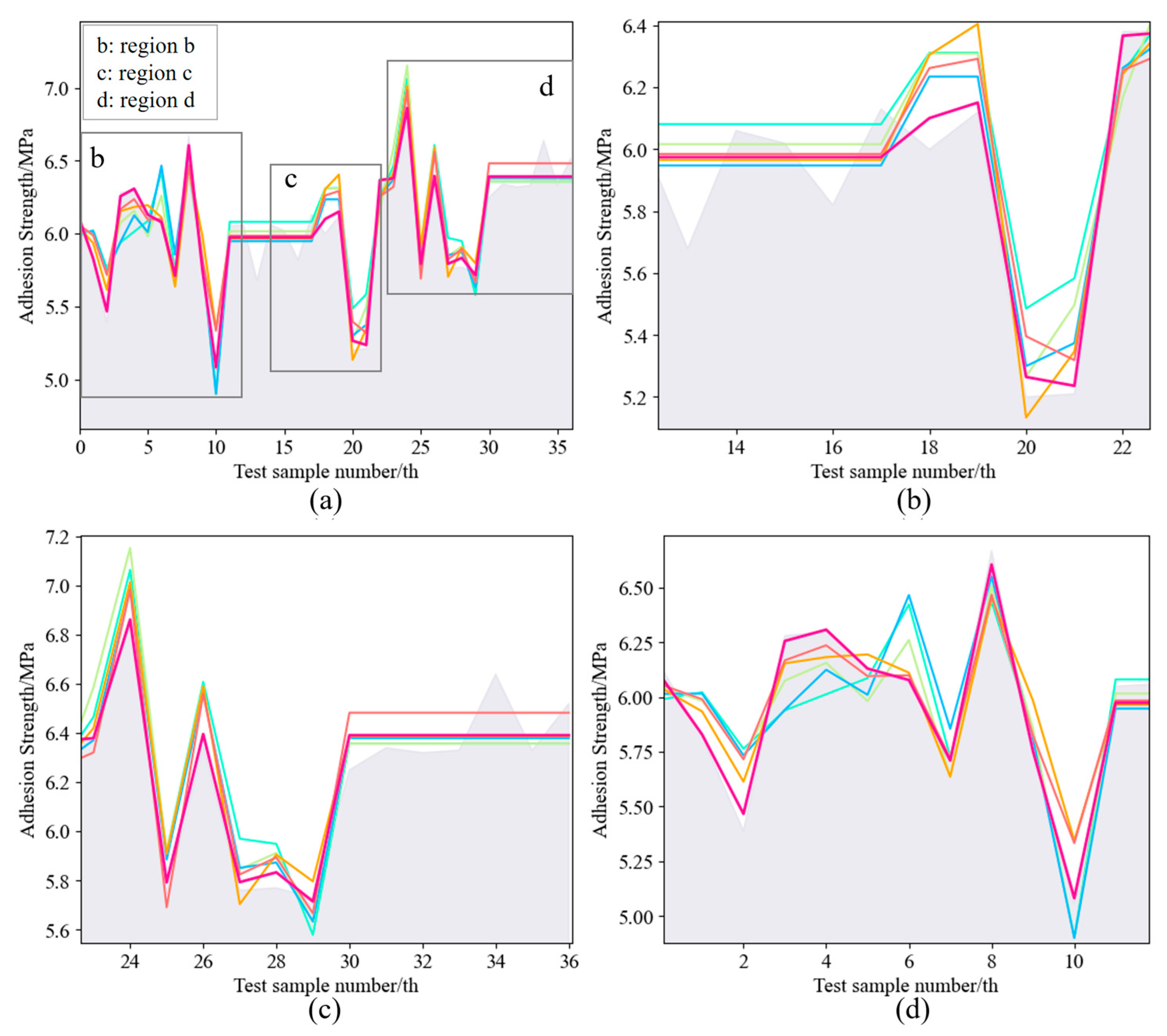
3.1. Data Preprocessing

The literature [52] provided the experimental data for this paper. In the literature, 186 groups of sylvestris pinus wood samples were tested for bond strength after treatment under different conditions. The specific data are provided in

Table A1. Wood treatment conditions and corresponding bond strength.

Treatment Temperature/°C	Treatment Time/h	Feed Rate/m/min	Cutting Speed/m/s	Grit Size	Adhesion Strength/MPa
190	2	16	4	100–150	5.54
210	2	16	4	100–150	5.96
190	2	16	6	100–150	5.94
210	2	16	6	100–150	5.64
190	2	20	4	100–150	7.26
210	2	20	4	100–150	6.83
190	2	20	6	100–150	6.17
210	2	20	6	100–150	5.48
190	4	16	4	100–150	5.02
210	4	16	4	100–150	5.04
190	4	16	6	100–150	5.93
210	4	16	6	100–150	6.17
190	4	20	4	100–150	5.86
210	4	20	4	100–150	6.17
190	4	20	6	100–150	5.99
210	4	20	6	100–150	6.05
180	3	18	5	100–150	6.45
220	3	18	5	100–150	6.15
200	3	18	3	100–150	6.34
200	3	18	7	100–150	6.11
200	3	14	5	100–150	4.95
200	3	22	5	100–150	6.15
200	1	18	5	100–150	5.71
200	5	18	5	100–150	5.17
200	3	18	5	100–150	5.75
200	3	18	5	100–150	5.59
200	3	18	5	100–150	5.94
200	3	18	5	100–150	6
200	3	18	5	100–150	6.04
200	3	18	5	100–150	5.96
200	3	18	5	100–150	6.15
190	2	16	4	100–150	6.18
210	2	16	4	100–150	5.76
190	2	16	6	100–150	5.68
210	2	16	6	100–150	5.95
190	2	20	4	100–150	7.56
210	2	20	4	100–150	7.09
190	2	20	6	100–150	6
210	2	20	6	100–150	5.78
190	4	16	4	100–150	4.38
210	4	16	4	100–150	5.14
190	4	16	6	100–150	6.23
210	4	16	6	100–150	5.79
190	4	20	4	100–150	6.11
210	4	20	4	100–150	5.95
190	4	20	6	100–150	5.96
210	4	20	6	100–150	5.82
180	3	18	5	100–150	6.89
220	3	18	5	100–150	5.84
200	3	18	3	100–150	5.65
200	3	18	7	100–150	6.04
200	3	14	5	100–150	5.77
200	3	22	5	100–150	6.48
200	1	18	5	100–150	5.94
200	5	18	5	100–150	4.56
200	3	18	5	100–150	5.94
200	3	18	5	100–150	5.56
200	3	18	5	100–150	5.99
200	3	18	5	100–150	6.08
200	3	18	5	100–150	6.16
200	3	18	5	100–150	5.64
200	3	18	5	100–150	6.11
190	2	16	4	100–150	6.04
210	2	16	4	100–150	5.58
190	2	16	6	100–150	6.05
210	2	16	6	100–150	5.79
190	2	20	4	100–150	7.09
210	2	20	4	100–150	6.78
190	2	20	6	100–150	5.79
210	2	20	6	100–150	5.31
190	4	16	4	100–150	4.97
210	4	16	4	100–150	5.06
190	4	16	6	100–150	5.84
210	4	16	6	100–150	6.01
190	4	16	4	100–120	6.67
210	2	16	4	100–120	6.41
190	2	16	6	100–120	6.05
210	2	16	6	100–120	5.62
190	2	20	4	100–120	7.01
210	2	20	4	100–120	6.91
190	2	20	6	100–120	5.17
210	2	20	6	100–120	4.74
190	4	16	4	100–120	6.33
210	4	16	4	100–120	5.84
190	4	16	6	100–120	6.76
210	4	16	6	100–120	6.49
190	4	20	4	100–120	6.24
210	4	20	4	100–120	6.29
190	4	20	6	100–120	5.57
210	4	20	6	100–120	5.26
180	3	18	5	100–120	6.62
220	3	18	5	100–120	6.29
200	3	18	3	100–120	7.1
200	3	18	7	100–120	5.44
200	3	14	5	100–120	6.45
200	3	22	5	100–120	5.97
200	1	18	5	100–120	5.64
200	5	18	5	100–120	5.44
200	3	18	5	100–120	6.45
200	3	18	5	100–120	6.22
200	3	18	5	100–120	5.97
200	3	18	5	100–120	6.37
200	3	18	5	100–120	6.25
200	3	18	5	100–120	6.7
200	3	18	5	100–120	6.33
190	2	16	4	100–120	6.81
210	2	16	4	100–120	6.85
190	2	16	6	100–120	6.83
210	2	16	6	100–120	6.36
190	2	20	4	100–120	7.08
210	2	20	4	100–120	7.1
190	2	20	6	100–120	5.43
210	2	20	6	100–120	4.95
190	4	16	4	100–120	6.15
210	4	16	4	100–120	5.93
190	4	16	6	100–120	6.74
210	4	16	6	100–120	6.63
190	4	20	4	100–120	6.67
210	4	20	4	100–120	6.42
190	4	20	6	100–120	5.48
210	4	20	6	100–120	4.94
180	3	18	5	100–120	6.52
220	3	18	5	100–120	6.22
200	3	18	3	100–120	7.26
200	3	18	7	100–120	5.8
200	3	14	5	100–120	6.84
200	3	22	5	100–120	5.84
200	1	18	5	100–120	5.96
200	5	18	5	100–120	5.48
200	3	18	5	100–120	5.95
200	3	18	5	100–120	6.42
200	3	18	5	100–120	6.41
200	3	18	5	100–120	6.64
200	3	18	5	100–120	6.55
200	3	18	5	100–120	6.34
200	3	18	5	100–120	6.36
190	2	16	4	100–120	6.89
210	2	16	4	100–120	6.76
190	2	16	6	100–120	6.31
210	2	16	6	100–120	6.12
190	2	20	4	100–120	7.73
210	2	20	4	100–120	7.06
190	2	20	6	100–120	5.74
210	2	20	6	100–120	4.95
190	4	16	4	100–120	5.63
210	4	16	4	100–120	5.93
190	4	16	6	100–120	6.81
210	4	16	6	100–120	6.7
190	4	20	4	100–120	5.86
210	4	20	4	100–150	6.14
190	4	20	6	100–150	5.82
210	4	20	6	100–150	5.39
210	3	18	5	100–150	6.28
190	3	18	5	100–150	6.3
210	3	18	3	100–150	6.13
180	3	18	7	100–150	6.07
220	3	14	5	100–150	5.71
200	3	22	5	100–150	6.67
200	1	18	5	100–150	5.74
200	5	18	5	100–150	5.06
200	3	18	5	100–150	6.05
200	3	18	5	100–150	6.06
200	3	18	5	100–150	5.68
200	3	18	5	100–150	6.06
200	3	18	5	100–150	6.02
200	3	18	5	100–150	5.82
200	3	18	5	100–150	6.13
200	4	20	4	100–120	6
200	4	20	4	100–120	6.12
200	4	20	6	100–120	5.2
190	4	20	6	100–120	5.21
210	3	18	5	100–120	6.38
190	3	18	5	100–120	6.38
210	3	18	3	100–120	6.85
180	3	18	7	100–120	5.75
220	3	14	5	100–120	6.35
200	3	22	5	100–120	5.76
200	1	18	5	100–120	5.77
200	5	18	5	100–120	5.73
200	3	18	5	100–120	6.25
200	3	18	5	100–120	6.34
200	3	18	5	100–120	6.32
200	3	18	5	100–120	6.33
200	3	18	5	100–120	6.64
200	3	18	5	100–120	6.33
200	3	18	5	100–120	6.52

of Appendix A.

In the experiment, 186 samples of sylvestris pinus wood with dimensions of 20 mm (height) × 120 mm (width) × 100 mm (length) were cut, and the samples were conditioned at 20 °C ± 2 °C and 65% ± 1% relative humidity to reach equilibrium moisture content, followed by heat treatment. The heat treatment temperature had five levels (180, 190, 200, 210, and 220 °C) and the heat treatment time had five levels (1, 2, 3, 4, and 5 h). The samples were then sanded under a tension of 3 kg/cm² and sandpaper type of aluminum oxide using a broadband sander with five levels of feed speed (3, 4, 5, 6, and 7 m/min), five levels of cutting speed (14, 16, 18, 20, and 22 m/s) and two levels of sandpaper grit (100–120 and 100–150). The samples were coated with water-based varnish using a pneumatic gun at 0.8 MPa pressure for the coating process. Finally, the bond strength was measured using the pull-off test method, which was performed according to ios 4624, using a PosiTest AT adhesion tester as the test instrument.

When using the IHHO-BP model to predict the bonding strength, we use the first 149 sets of data (approximately 80%) from Table A1 in the Appendix A as the training set, and the remaining 37 sets of data (approximately 20%) serve as the test set [52]. Since the data sizes differ between the five input dimensions of the model, the input data are normalized by Equation (21) in this paper to avoid the large difference in data sizes between the input dimensions from affecting the prediction model’s convergence speed and training accuracy:

$$y=\left(y_{max}-y_{min}\right)\times {\displaystyle \frac{x-x_{min}}{x_{max}-x_{min}}}+y_{min}$$

(21)

The normalized value of $x$, denoted by $y$, with $x_{min}$ and $x_{max}$ being the minimum and maximum values, respectively, and the normalization interval $[y_{min}, y_{max}]$ is set to $[0, 1]$.

3.2. Model Parameter Settings

3.2.1. Metaheuristic Algorithm Parameter Settings

In order to evaluate the effectiveness of the IHHO algorithm, we compare it not only with the original HHO algorithm but also with some commonly used metaheuristic algorithms (MA): Genetic Algorithm (GA), Particle Swarm Optimization (PSO), and Whale Optimization Algorithm (WOA). The corresponding parameter settings for each meta-heuristic algorithm are shown in

Table 1. MHAs’ parameters setting.

Algorithm	Parameter	Setting
GA	$a$	0.8
	$b$	0.05
PSO	$C_1$ and $C_2$	2
	Inertia weight	Linearly decreased from 0.9 to 0.1
WOA	$a$	Gradually Reduced from 2 to 0
HHO	escape energy factor $E$	Linearly decreased from 1 to −1
IHHO	escape energy factor $E$	Linearly decreased from 1 to −1
	The dimension of the Sobol sequence $d$	64
	Probability of t-distribution perturbation $p$	0.5

. To ensure fairness, the maximum number of iterations and the population size for each meta-heuristic algorithm are set to 100 and 50, respectively.

3.2.2. Determination of the Number of Neurons and Activation Function in the Model

In this study, the BP neural network within the IHHO-BP framework adopts a triple-layer architecture consisting of an input layer, a hidden layer, and an output layer. The number of nodes in the input layer is five, corresponding to the input data of heat treatment temperature, heat treatment time, feed rate, cutting speed, and gravel size. The output layer consists of a single node, representing the bonding strength of the wood. The maximum number of iterations for the BP neural network model is fixed at 1000, with a target error of 0.0001, and a learning rate of 0.01 [25].

Establishing the neuron count (number of nodes within the hidden layer) in the BP framework is a critical step in constructing an efficient neural network. The neuron count within the hidden layer directly affects the framework’s learning ability and generalization performance. Too few neurons may lead to underfitting of the model, unable to capture complex patterns in the data; too many neurons may lead to overfitting of the model, performing well on training data but poorly on new data. Therefore, reasonably determining the neuron count within the hidden layer is crucial for building an efficient and robust BP model. The number of nodes in the neural network hidden layer is usually determined based on empirical Equation (22), so the range of choices for the number of nodes in the hidden layer in this paper is [4,13]:

$$q=\sqrt{\left(u+v\right)}+w, w\in \left(1, 10\right)$$

(22)

where $q$, $u$, and $v$ represent the number of nodes in the hidden layer, the input layer, and the output layer, respectively.

Simultaneously, determining the activation function of the BP neural network model is also one of the key steps in building an efficient neural network. Activation functions play a crucial role in BP neural network models as they introduce nonlinearity, enabling the neural network to learn and represent complex patterns and relationships. Without activation functions, the neural network would only be able to represent linear transformations, greatly limiting its expressive power. Commonly used activation functions in the BP model include: tansig, relu, sigmoid, and purelin. Since the hidden layer usually performs complex calculations, nonlinear activation functions such as tansig, relu, and sigmoid are often chosen to augment the network’s capacity to emulate complex data relationships. The activation function for the output layer is usually chosen based on specific tasks, with sigmoid and purelin being commonly used.

In

Table A2. Hidden layer neuron number and optimal activation function evaluation results.

Number of Hidden Layer Neurons	Activate Functions	Average Score	First-Fold Score	Second-Fold Score	Third-Fold Score	Fourth-Fold Score	Fifth-Fold Score
4	tansig-purelin	0.1844	0.2045	0.1610	0.2226	0.1640	0.1696
	tansig-sigmod	0.1946	0.2274	0.2162	0.1225	0.2068	0.2003
	sigmod-purelin	0.1326	0.1332	0.1238	0.1446	0.1359	0.1254
	sigmod-sigmod	0.1619	0.1343	0.1233	0.2270	0.1324	0.1923
	relu-purelin	0.1562	0.1817	0.1352	0.1301	0.1824	0.1515
	relu-sigmod	0.1755	0.1910	0.2116	0.1466	0.1717	0.1564
5	tansig-purelin	0.0691	0.0557	0.0785	0.0692	0.0768	0.0656
	tansig-sigmod	0.0786	0.0618	0.0833	0.0824	0.0829	0.0828
	sigmod-purelin	0.0742	0.0635	0.0839	0.0807	0.0695	0.0733
	sigmod-sigmod	0.0732	0.0794	0.0544	0.0876	0.0643	0.0805
	relu-purelin	0.0738	0.0802	0.0590	0.0634	0.0781	0.0885
	relu-sigmod	0.0731	0.0629	0.0852	0.0790	0.0730	0.0654
6	tansig-purelin	0.0464	0.0483	0.0533	0.0419	0.0444	0.0441
	tansig-sigmod	0.0475	0.0409	0.0473	0.0505	0.0574	0.0412
	sigmod-purelin	0.0534	0.0495	0.0431	0.0564	0.0589	0.0593
	sigmod-sigmod	0.0513	0.0566	0.0458	0.0579	0.0518	0.0444
	relu-purelin	0.0459	0.0449	0.0429	0.0416	0.0542	0.0461
	relu-sigmod	0.0518	0.0574	0.0598	0.0501	0.0412	0.0507
7	tansig-purelin	0.0426	0.0371	0.0583	0.0352	0.0463	0.0361
	tansig-sigmod	0.0499	0.0439	0.0405	0.0497	0.0581	0.0573
	sigmod-purelin	0.0442	0.0424	0.0471	0.0381	0.0389	0.0547
	sigmod-sigmod	0.0468	0.0580	0.0442	0.0333	0.0415	0.0568
	relu-purelin	0.0523	0.0588	0.0583	0.0489	0.0366	0.0587
	relu-sigmod	0.0509	0.0419	0.0414	0.0580	0.0576	0.0556
8	tansig-purelin	0.0453	0.0510	0.0416	0.0469	0.0385	0.0484
	tansig-sigmod	0.0468	0.0495	0.0536	0.0359	0.0541	0.0410
	sigmod-purelin	0.0450	0.0348	0.0517	0.0353	0.0444	0.0588
	sigmod-sigmod	0.0451	0.0404	0.0574	0.0416	0.0308	0.0550
	relu-purelin	0.0392	0.0355	0.0310	0.0473	0.0431	0.0390
	relu-sigmod	0.0465	0.0562	0.0336	0.0500	0.0531	0.0396
9	tansig-purelin	0.0244	0.0191	0.0350	0.0325	0.0175	0.0177
	tansig-sigmod	0.0253	0.0273	0.0306	0.0247	0.0239	0.0202
	sigmod-purelin	0.0275	0.0250	0.0266	0.0188	0.0311	0.0359
	sigmod-sigmod	0.0264	0.0339	0.0301	0.0212	0.0214	0.0251
	relu-purelin	0.0251	0.0257	0.0197	0.0344	0.0271	0.0184
	relu-sigmod	0.0272	0.0312	0.0245	0.0328	0.0288	0.0185
10	tansig-purelin	0.0282	0.0299	0.0296	0.0228	0.0299	0.0285
	tansig-sigmod	0.0363	0.0327	0.0323	0.0362	0.0386	0.0418
	sigmod-purelin	0.0347	0.0431	0.0267	0.0457	0.0201	0.0377
	sigmod-sigmod	0.0313	0.0204	0.0447	0.0288	0.0407	0.0221
	relu-purelin	0.0395	0.0346	0.0270	0.0472	0.0408	0.0479
	relu-sigmod	0.0313	0.0427	0.0270	0.0270	0.0358	0.0242
11	tansig-purelin	0.0382	0.0480	0.0366	0.0377	0.0282	0.0405
	tansig-sigmod	0.0381	0.0437	0.0324	0.0362	0.0320	0.0460
	sigmod-purelin	0.0379	0.0357	0.0314	0.0390	0.0430	0.0405
	sigmod-sigmod	0.0341	0.0424	0.0316	0.0353	0.0245	0.0364
	relu-purelin	0.0309	0.0256	0.0325	0.0285	0.0422	0.0258
	relu-sigmod	0.0320	0.0344	0.0309	0.0257	0.0264	0.0423
12	tansig-purelin	0.0289	0.0252	0.0236	0.0299	0.0358	0.0300
	tansig-sigmod	0.0331	0.0317	0.0365	0.0410	0.0316	0.0246
	sigmod-purelin	0.0384	0.0327	0.0476	0.0437	0.0434	0.0245
	sigmod-sigmod	0.0318	0.0259	0.0331	0.0328	0.0288	0.0384
	relu-purelin	0.0317	0.0306	0.0255	0.0450	0.0353	0.0222
	relu-sigmod	0.0347	0.0277	0.0313	0.0407	0.0408	0.0331
13	tansig-purelin	0.0305	0.0402	0.0243	0.0280	0.0236	0.0361
	tansig-sigmod	0.0357	0.0403	0.0381	0.0303	0.0251	0.0445
	sigmod-purelin	0.0309	0.0335	0.0229	0.0273	0.0298	0.0412
	sigmod-sigmod	0.0382	0.0413	0.0311	0.0365	0.0478	0.0342
	relu-purelin	0.0384	0.0368	0.0336	0.0469	0.0435	0.0309
	relu-sigmod	0.0328	0.0278	0.0474	0.0256	0.0389	0.0241

of Appendix A, we use the Root Mean Square Error (RMSE) as the evaluation metric and determine the optimal neuron count for the hidden layer and their corresponding activation function combinations through five-fold cross-validation. The smaller the RMSE as an error indicator, the better the model performs on the given dataset. As can be seen from Table A2 in Appendix A, in this experiment, the optimal neuron count for the hidden layer is nine, and the corresponding optimal activation function combination is tansig for the hidden layer and purelin for the output layer.

3.2.3. Evaluation Criteria of the Model

In this paper, we select the mean square error (MSE), mean absolute error (MAE), RMSE, mean absolute percentage error (MAPE), and coefficient of determination ($R^2$) as indicators for evaluating the model’s accuracy and precision. These indicators are calculated as Equations (23)–(26):

$$MAE={\displaystyle \frac{1}{n}}{\sum }_{t=1}^n\left|A_t-F_t\right|$$

(23)

$$RMSE=\sqrt{{\displaystyle \frac{1}{n}}{\sum }_{t=1}^n{\left(A_t-F_t\right)}^2}$$

(24)

$$MAPE={\displaystyle \frac{1}{n}}{\sum }_{t=1}^n\left|{\displaystyle \frac{A_t-F_t}{A_t}}\right|\times 100\%$$

(25)

$$R^2=1-{\displaystyle \frac{{\sum }_{t=1}^n{\left(A_t-F_t\right)}^2}{{\sum }_{t=1}^n{\left(A_t-F_t\right)}^2}}$$

(26)

where $A_t$ and $F_t$ are the values observed and estimated by the model, respectively, and $n$ is the total number of samples.

4. Results and Discussion

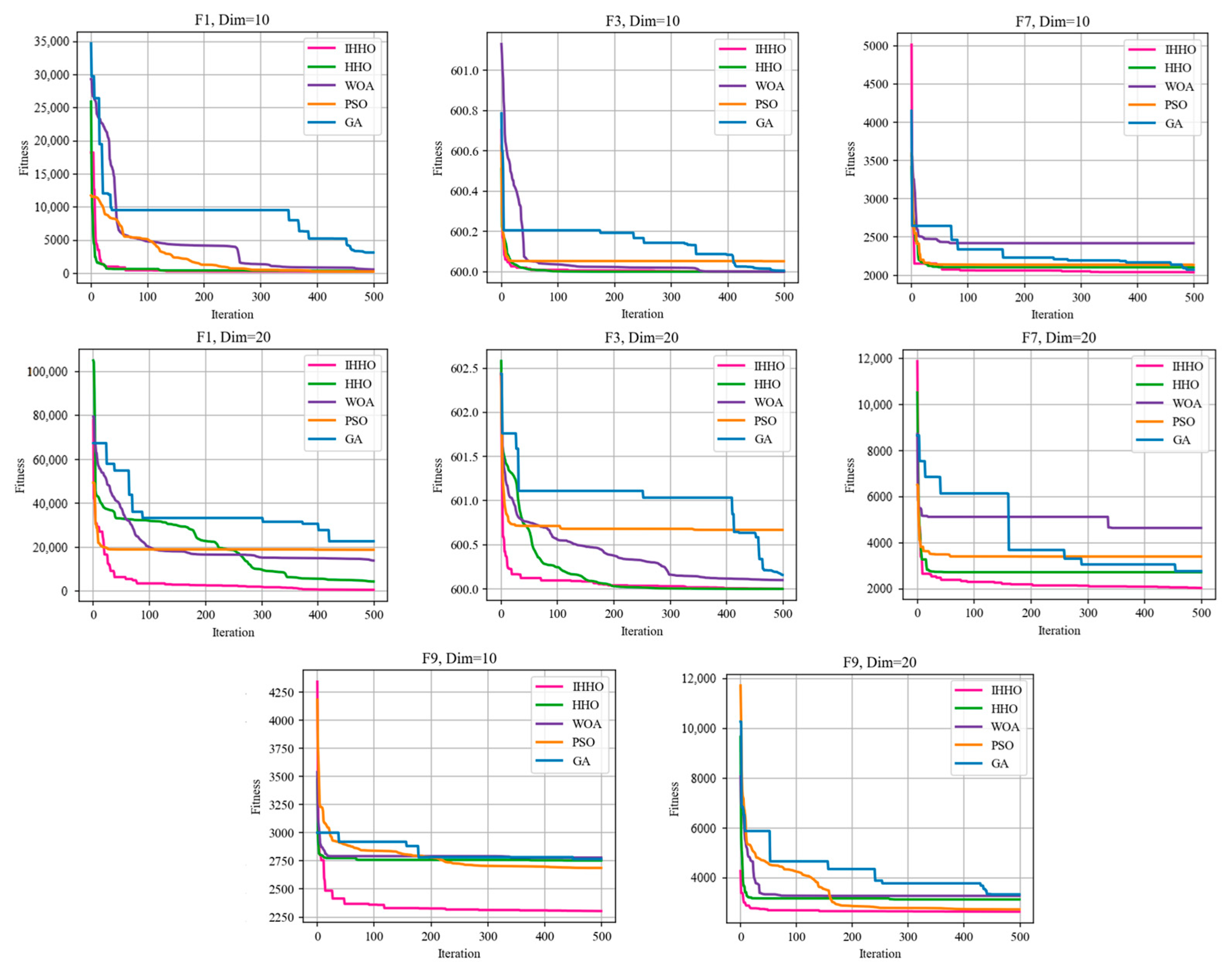
4.1. Verification of the Effectiveness of the IHHO Algorithm

To impartially evaluate the performance of IHHO and verify the effectiveness of IHHO’s improvement strategies, four benchmark test functions were carefully selected from the CEC2022 test function set for performance testing. These include the unimodal function F1, which has only one optimal solution, and is used to measure the convergence speed and optimization ability of the method; the multi-peak function F3, which has several optimal solutions, and is utilized to evaluate the method’s capacity to escape local optima and its exploration ability; the hybrid function F7, which contains multiple subfunctions, and is employed to evaluate the method’s capacity to escape local optima; and the composite function F9, each of the subfunctions of which has additional bias values and weights, further increasing the difficulty of solving the optimization algorithm. Each test function is chosen in two different dimensions, i.e., 10-dimensional and 20-dimensional, to test the algorithm’s solving ability in low and high dimensions. The specific information of the selected test functions is shown in

Table 2. Specific Information of the test functions.

Function	Formula	Dim	Search Range	Best Value
F1	$f(x)={\sum }_{i=1}^D{x}_i^2+{({\sum }_{i=1}^{D}0.5x_i)}^2+{({\sum }_{i=1}^{D}0.5x_i)}^4$	10/20	[−100, 100]	300
F3	$f(x)=g(x_1,x_2)+g(x_2,x_3)+\dots +g(x_{D-1},x_D)+g(x_D,x_1)$ $g(x,y)+0.5+{\displaystyle \frac{({\sin }^2(\sqrt{x^2+y^2})-0.5)}{{(1+0.001(x^2+y^2))}^2}}$	10/20	[−100, 100]	600
F7	$f(x)={\left|{({\sum }_{i=1}^D{x}_i^2)}^2-{({\sum }_{i=1}^D{x}_i)}^2\right|}^{0.5}+(0.5{\sum }_{i=1}^D{x}_i^2+{\sum }_{i=1}^D{x}_i)/D+0.5$	10/20	[−100, 100]	2000
F9	$f(x)={\displaystyle \frac{10}{D^2}}{\prod }_{1=1}^D{(1+i{\sum }_{j=1}^{32}{\displaystyle \frac{\left|2^j{x}_i-round(2^j{x}_i)\right|}{2^j}})}^{{\displaystyle \frac{10}{D^{1.2}}}}-{\displaystyle \frac{10}{D^2}}$	10/20	[−100, 100]	2300

.

In the experiment, the IHHO algorithm was compared not only with the unimproved HHO algorithm, but also with classic swarm intelligence optimization algorithms, including GA [28], PSO [29], and WOA [30]. The population size, maximum number of iterations, and number of independent runs for each algorithm were all set to 30, 500, and 30, respectively. The optimal value, maximum value, mean value, and standard deviation of the outcomes of 30 runs of each algorithm were calculated. The convergence curves of each algorithm are shown in Figure 7. The final optimization outcomes are presented in

Table 3. Solution results of each algorithm on test functions of different dimensions.

Function	Dim	Indicator	IHHO	HHO	WOA	PSO	GA
F1	10	Best	300.3694	301.6383	313.8464	311.0403	322.0550
		Average	335.9410	403.9251	431.5243	439.9808	504.5946
		STD	21.3837	64.2540	78.1941	91.7957	107.2404
	20	Best	328.1572	652.4272	991.6811	1829.4519	2726.1598
		Average	1231.8510	2657.4552	8038.1607	8256.8382	11,244.2925
		STD	1141.5671	1313.5080	4567.1136	5003.6406	5699.8139
F3	10	Best	600.0000	600.0003	600.0009	600.0010	600.0161
		Average	600.0026	600.0078	600.0296	600.0423	600.1232
		STD	0.0056	0.0105	0.0258	0.0294	0.0699
	20	Best	600.0001	600.0004	600.0886	600.0955	600.3625
		Average	600.0028	600.0307	600.3321	600.3737	600.6267
		STD	0.0017	0.0177	0.1464	0.1830	0.2012
F7	10	Best	2038.7114	2052.2212	2059.4569	2073.7016	2051.6123
		Average	2096.6045	2120.9077	2192.6254	2328.8584	2459.1100
		STD	39.1627	46.1024	98.9004	174.5463	296.0627
	20	Best	2047.6545	2090.5460	2894.7576	2684.4154	2889.1896
		Average	2153.6233	2968.4444	3500.9027	3985.8512	4607.1419
		STD	60.3008	483.1014	407.6184	744.7080	978.4388
F9	10	Best	2301.1321	2327.4268	2331.9077	2357.1124	2340.4099
		Average	2529.3670	2667.2676	2740.4971	2812.9339	2754.3577
		STD	159.0777	171.9700	234.9014	250.3330	285.7676
	20	Best	2382.9228	2499.3693	2749.4379	2938.4243	3029.0854
		Average	2720.9958	2735.8546	3016.1995	3265.8828	3346.1276
		STD	178.5477	186.5087	204.1760	207.5216	215.7812

.

Figure 7 intuitively displays the convergence curves of each algorithm on different dimensions and test functions. From this, we can observe that IHHO demonstrates the fastest convergence speed and the highest convergence accuracy among the selected test functions. Its convergence process is almost linear, showing superior convergence speed. For the GA, PSO, WOA, and HHO algorithms, it can be observed that when the IHHO algorithm iterates near the optimal solution, the other algorithms are still iterating towards the optimal solution, demonstrating the superior convergence speed of IHHO. At the same time, for these test functions, especially when the function dimension is 20, IHHO can get very close to the optimal solution after reaching the final number of iterations, while some other algorithms still have a large gap with the optimal solution after reaching the final number of iterations. This once again highlights the superior fitting accuracy of IHHO, and indicates that IHHO can maintain good solution accuracy and stability in solving high-dimensional problems. As can be seen from Figure 7, during the testing process, the GA often stops iterating in the early stages before finding the optimal solution, and then starts iterating again in the later stages. This indicates that the GA is easily influenced by local optima. The PSO algorithm also sometimes stops iterating in the early stages before finding the optimal solution, and does not update iterations in the later stages. This suggests that the PSO algorithm may fall into local optima, thereby affecting the accuracy of the solution. The WOA performs well on other test functions but not so well on test function F7. F7, which includes multiple subfunctions, is also commonly used to test the ability of algorithms to escape local optima. This indicates that WOA is also influenced by local optima, leading to a decrease in the accuracy of the solution.

As can be seen from Table 3, IHHO leads in the optimal value, average value, and standard deviation of the optimization results across all test functions of different dimensions selected, demonstrating superior convergence accuracy and highlighting its stability and efficiency in solving high-dimensional problems. At the same time, IHHO’s test results on the selected test functions are overall better than WOA, PSO, and GA. The results show that IHHO surpasses HHO in terms of performance in developing optimal solutions, verifying the effectiveness of the improvement strategies in enhancing the search and exploration capabilities of the original algorithm.

4.2. Comparison Results with Other Benchmark Models

From the algorithm’s performance on the test functions, we understand that the improved IHHO algorithm demonstrates superior convergence speed and solution accuracy, and exhibits good solution stability on high-dimensional problems. In this section, the BP model optimized by the IHHO algorithm, namely the IHHO-BP model, is employed to estimate the bonding strength of timber, and is contrasted against the HHO-BP, WOA-BP, PSO-BP, GA-BP, and BP benchmark models to verify the effectiveness of the wood bonding strength prediction model proposed in this paper. The fitting curve of the predicted bonding strength values and actual values of each model is shown in Figure 8.

As can be intuitively seen from Figure 8, overall, the predicted values of wood bonding strength by the IHHO-BP model are closest to the actual values, outperforming the HHO-BP, WOA-BP, PSO-BP, and BP models. This indicates that the model can achieve superior prediction accuracy. Looking at it locally, the predicted values of the IHHO-BP model are also more closely aligned with the actual values. Among the benchmark models compared, the HHO-BP model has a slightly better fit between the predicted values and actual values than the WOA-BP and PSO-BP models. However, there is a significant gap between the predicted values and actual values of the original BP model. This suggests that the hyperparameters randomly generated by the original BP can have some adverse effects on the prediction model, and it is valuable to optimize it using the original heuristic algorithm.

Then, the model is evaluated more accurately through four evaluation metrics: MAE, RMSE, MAPE, and R². The results of each evaluation metric are visualized in Figure 9, and the specific results for each assessment metric are presented in

Table 4. Evaluation metrics for each model.

Model	MAE/MPa	RMSE/MPa	MAPE/%	R2
BP	0.1709	0.2076	2.8811	0.7363
GA-BP	0.1488	0.1757	2.4852	0.8112
PSO-BP	0.1459	0.1691	2.4414	0.8250
WOA-BP	0.1370	0.1581	2.2926	0.8470
HHO-BP	0.1316	0.1534	2.2123	0.8559
IHHO-BP	0.0643	0.0915	1.0635	0.9488

.

The smaller the error indicators MAE, RMSE, and MAPE, the smaller the gap between the model’s predicted values and the actual values, indicating higher prediction accuracy and better performance of the model. The coefficient of determination R² typically ranges from 0 to 1, and the closer R² is to 1, the better the fit between the model’s predicted values and actual values, indicating higher prediction accuracy. As depicted in Figure 9, the MAE, RMSE, and MAPE of the IHHO-BP model are 0.0643, 0.0915, and 1.0635%, respectively, which are significantly smaller than those of other comparison models, demonstrating superior prediction accuracy. The R² of the IHHO-BP model reached 0.9488, which is closer to 1 compared to other comparison models, indicating that the IHHO-BP model has a better fit.

Table 4 presents the specific information of various evaluation metrics for different models. It can be observed that the predictive performance of BP has been enhanced to different extents through optimization by different meta-heuristic algorithms. However, in forecasting the bonding strength of heat-treated timber, the IHHO-BP model performs the best among all comparison models. Compared with the HHO-BP model, the MAE, RMSE, MAPE, and R² of the IHHO-BP model have improved by 51.16%, 40.38%, 51.93%, and 10.85%, respectively. This indicates that the HHO algorithm, improved by the Sobol sequence, Whale Optimization Algorithm, and t-distribution perturbation, has better optimization capabilities, can better optimize the hyperparameters of the BP model, and thus, makes the IHHO-BP model more adaptable to the task of predicting the bonding strength of heat-treated wood. At the same time, it also proves the effectiveness of the three improvement measures proposed in this paper for the HHO algorithm, the superiority of the IHHO algorithm, and the superiority of IHHO-BP in forecasting the bonding strength of heat-treated timber. Meanwhile, compared with the WOA-BP, PSO-BP, GA-BP, and original BP models, the IHHO-BP model has further optimized MAE, RMSE, MAPE, and R² by 53.08%, 42.16%, 53.61%, and 12.02%; 55.95%, 45.90%, 56.44%, and 15.00%; 56.81%, 47.93%, 57.21%, and 16.96%; and 62.38%, 55.94%, 63.09%, and 28.86%, respectively. This once again highlights the superiority of the IHHO-BP model in predicting the bonding strength of heat-treated wood.

The significant gap between the performance of BP and the other models can be attributed to the fact that the hyperparameters of the original BP are randomly generated. This randomness greatly limits the efficiency and accuracy of the prediction process. The differences in the results of the other algorithms are mainly due to the varying optimization capabilities of the different algorithms. It can be concluded that in the field of predicting the bonding strength of heat-treated wood, the optimization capability of the HHO algorithm is superior to the other compared metaheuristic algorithms. This conclusion is consistent with the results obtained from our function tests. The superior performance of the IHHO algorithm over the HHO algorithm can be attributed to the three-point improvement strategy we implemented: initializing the population using the Sobol sequence, updating the HHO position in combination with the WOA algorithm, and using a t-distribution perturbation to prevent the algorithm from falling into local optima. These improvements have effectively enhanced the optimization capability of the HHO algorithm.

Firstly, the IHHO algorithm initializes the population using the Sobol sequence. The Sobol sequence is a low-discrepancy sequence that can generate uniformly distributed sample points. This uniformly distributed initial population helps cover a wider search space, ensuring that the algorithm can fully explore the possible solution space at the beginning of the search, avoiding the initial population concentrating in certain local areas, thereby improving the algorithm’s global search capability. This uniform distribution characteristic gives the algorithm good diversity at the initial stage, laying a solid foundation for subsequent optimization processes.

Secondly, the IHHO algorithm combines the global search advantage of the Whale Optimization Algorithm (WOA). The Whale Optimization Algorithm, by simulating the predation behavior of humpback whales, has a strong global search capability. In the IHHO algorithm, WOA is used to update the position of the Harris hawk population, significantly enhancing the ability of the population to find the optimal solution globally. Specifically, WOA uses two mechanisms, spiral updating and encircling predation, to enable the population to search globally. In this way, the IHHO algorithm can perform better global searches, find more optimal hyperparameter combinations, and thereby improve the predictive performance of the model.

Finally, the IHHO algorithm uses t-distribution perturbation to perturb the Harris hawk population. The t-distribution, as a probability distribution with a larger tail, can introduce a moderate degree of randomness during the search process. By perturbing the population with a t-distribution, the IHHO algorithm can introduce appropriate mutations during the local development process, enhancing the population’s development capability. This perturbation mechanism not only helps avoid the algorithm falling into local optimal solutions but also maintains the diversity of the population during the search process, thereby improving the predictive performance of the model.

4.3. Comparison with Previous Research Results

To further evaluate the proposed IHHO-BP model for predicting the bonding strength of heat-treated wood, this paper also compares it with previous research. We compared several models that have been used for wood bonding strength prediction, including Linear Regression (LR), Extreme Learning Machine (ELM), Support Vector Regression (SVR), GA-optimized Support Vector Regression (GA-SVR) [52], and Carnivorous Plant Algorithm-optimized BP (CPA-BP) [53].

LR is a linear model, the core concept of which is to establish a linear correlation model between the dependent variable and the independent variable, with the aim of minimizing the total error between the predicted value and the actual value. ELM is a nonlinear model that randomly initializes the connection weights from the input layer to the hidden layer and the weights from the hidden layer to the output layer, using the input to perform nonlinear fitting to the output. SVR, as a regression model based on Support Vector Machine (SVM), finds an optimal hyperplane in two-dimensional space to model the regression process. In the GA-SVR model, researchers use GA to optimize the penalty coefficient and kernel parameters of SVR. In the CPA-BP model, researchers use CPA to optimize the weights and thresholds of the BP model.

Table 5. Comparison with previous research results.

Model	MAE/MPa	RMSE/MPa	MAPE/%	R2
LR	0.2791	0.3535	4.7352	0.2548
ELM	0.2061	0.2672	3.3059	0.5958
SVR	0.1770	0.2047	2.7098	0.7340
GA-SVR	0.1439	0.1718	2.5143	0.8117
CPA-BP	0.1216	0.1326	2.0442	0.8927
IHHO-BP	0.0643	0.0915	1.0635	0.9488

shows the comparative analysis results of the IHHO-BP model with the above models.

Table 5 displays the evaluation metrics of each model. It can be seen that the LR model has the highest MAE, RMSE, and MAPE values, and the lowest R² value, indicating that among all the comparison models, the LR model has the lowest prediction accuracy and the worst fitting effect, making it challenging to meet the accuracy requirements for predicting the bonding strength of heat-treated wood. This may be due to the LR model assuming a linear relationship between the independent and dependent variables, and it cannot effectively handle the nonlinear relationships in the data of the bonding strength of heat-treated wood, leading to unsatisfactory prediction results.

Secondly, the ELM model also has a large error. Its poor prediction performance may be related to the fact that the weights and thresholds of the ELM model are randomly generated. In addition, the ELM model lacks the ability to adjust weights and thresholds through a backpropagation mechanism during the prediction process, making it difficult to effectively reduce prediction errors.

The prediction outcomes of the SVR model are similar to those of the BP neural network model. However, the prediction results of the GA-SVR model based on genetic algorithms are significantly better than the SVR model and are comparable to the GA-BP model. The similarity of the prediction results of the SVR model and the BP model may be due to the advantage of SVR in handling nonlinear relationships, but its performance depends on the choice of hyperparameters, such as the type of kernel function, penalty parameters, and kernel parameters. If these parameters are not optimized, the prediction performance of SVR may be limited. In contrast, the GA-SVR model optimizes the hyperparameters of SVR through genetic algorithms, significantly improving the model’s predictive performance.

The CPA-BP model has significantly improved prediction performance compared to the original BP model, indicating that using meta-heuristic algorithms to optimize the hyperparameters of the BP model can effectively improve the model’s predictive performance. In addition, the predictive performance of the IHHO-BP framework is superior to the CPA-BP framework, further proving the superiority of the improved IHHO algorithm in optimizing the BP model. The performance improvement of the CPA-BP model can be attributed to the effective adjustment of the BP model’s hyperparameters during the optimization process by the CPA algorithm. By simulating the predation process of carnivorous plants, the CPA algorithm can find an optimal combination of hyperparameters in a larger search space, thereby improving the model’s prediction accuracy.

However, despite the excellent performance of the CPA-BP model, the predictive performance of the IHHO-BP model is more prominent, mainly due to three improvements in the IHHO algorithm.

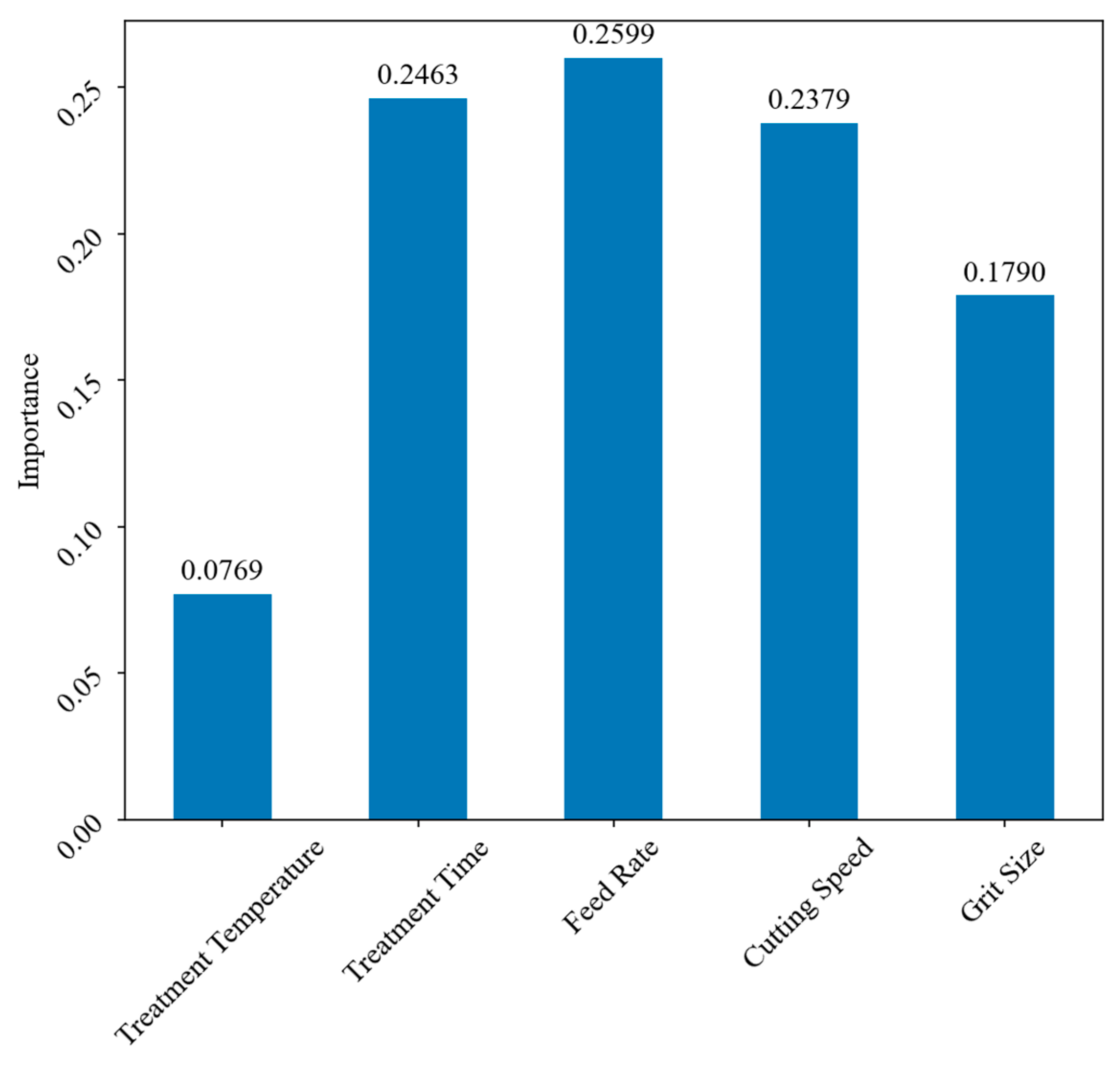
4.4. Analysis of Input Feature Importance

Feature importance analysis provides insights into which features contribute most significantly to the prediction outcome. In the context of predicting the bonding strength of heat-treated wood, this analysis allows us to identify the key factors that influence the bonding strength. Moreover, feature importance analysis can also help us understand the sensitivity of the prediction outcome to changes in the input features. This understanding can guide us in fine-tuning the input parameters to achieve optimal prediction results.

The Random Forest (RF) model is renowned for its robustness and versatility in handling various types of data. One of its key advantages is its ability to provide an analysis of feature importance [37,53]. This capability allows us to gain insights into the contribution of each feature to the prediction outcome, thereby enhancing our understanding of the prediction process. In our study, we used the RF model to analyze the importance of various input parameters in predicting the bonding strength of heat-treated wood. These parameters include treatment temperature, treatment time, feed rate, cutting speed, and grit size. To better calculate the contribution rate of each feature, we set the range of feature importance to be between 0 and 1. The results of the importance analysis for each input feature are shown in Figure 10.

As shown in Figure 10, the importance of the five input features in predicting the bonding strength of heat-treated wood varies.

Feed rate: with an importance score of 25.99%, feed rate is the most significant feature. This high importance suggests that the rate at which the wood is fed into the machine during the heat treatment process has a substantial impact on the bonding strength. This could be due to the fact that a faster feed rate might lead to less exposure to heat, thereby affecting the bonding strength. This finding underscores the need for careful control and optimization of the feed rate during the heat treatment process.

Treatment time: the second most important feature is the treatment time, with an importance score of 24.63%. This indicates that the duration of heat treatment also plays a crucial role in determining the bonding strength. Longer treatment times might allow for more thorough heat penetration, leading to stronger bonds. However, excessively long treatment times could potentially degrade the wood, highlighting the need for a balanced approach.

Cutting speed and grit size: the cutting speed and grit size have importance scores of 23.79% and 17.90%, respectively. The cutting speed’s importance suggests that the speed at which the wood is cut can influence the bonding strength, possibly by affecting the smoothness and uniformity of the cut surfaces. The grit size’s importance indicates that the size of the abrasive particles used in the sanding process can affect the bonding strength, likely by influencing the surface roughness.

Treatment temperature: the treatment temperature has the lowest importance score of 7.69%. While this might seem counterintuitive, as one might expect the temperature to have a significant impact on the heat treatment process, it suggests that within the range of temperatures considered in this study, the temperature has a relatively smaller influence on the bonding strength compared to the other factors. This could be due to a plateau effect, where beyond a certain temperature, further increases do not significantly improve the bonding strength.

5. Conclusions

Most current methods of measuring wood bond strength use the pull-off method, which is time-consuming and destructive and requires the use of a pull-off tester. Therefore, it is important to establish an effective model that can estimate the bond strength of wood accurately to reduce the cost and consumption of wood products in the production process and improve production efficiency. This paper developed the IHHO-BP prediction model to estimate the bond strength of 186 groups of heat-treated camphor pine wood based on five input variables: heat treatment temperature, heat treatment time, feed rate, cutting speed, and grit size. Of these groups, 149 were used as the training set and 37 as the test set. The main conclusions are summarized below.

• The IHHO algorithm is introduced to address the issue of the traditional HHO algorithm having limited global search ability and being prone to a local optimum. First, the population is initialized by using the Sobol sequence to improve the diversity of the initialized population and the uniformity of its distribution. Second, the population position is updated by integrating the Whale Optimization Algorithm to enhance the global search ability of the algorithm. Finally, t-distribution perturbation is incorporated to achieve a balance between the global search ability and exploitation ability of the algorithm to prevent the algorithm from converging to locally optimal solutions.
• We established the IHHO-BP model to forecast the bonding strength of heat-treated wood based on the heat treatment temperature, heat treatment time, feed speed, cutting speed, and sandpaper granularity. The proposed model was evaluated by comparing the prediction results with those of the HHO-BP, WOA-BP, PSO-BP, GA-BP, and BP models. The results showed that the IHHO-BP model had the smallest MAE, RMSE, and MAPE, and the largest R². This indicates that the IHHO-BP model has the smallest prediction error and superior prediction accuracy, and it can better meet the accuracy requirements for predicting the bonding strength of heat-treated wood.
• The IHHO-BP model was compared with previous LR, ELM, SVR, GA-SVR, and CPA-BP prediction models. The results showed that compared with the above models, the IHHO-BP model also achieved the lowest MAE, RMSE, and MAPE, and the highest R², once again highlighting the superior performance of the IHHO-BP model in forecasting the bonding strength of heat-treated wood.
• Through the importance analysis of five features in predicting the bonding strength of heat-treated wood using RF, it is concluded that in this study, feed rate has the greatest impact on the prediction of bonding strength, followed by treatment time, cutting speed, and grit size. Treatment temperature has the least impact on the prediction of bonding strength. This provides important reference for the study of factors affecting the bonding strength of heat-treated wood.
• However, this study has some limitations. Although we used evaluation metrics and compared multiple benchmark models to demonstrate the superiority of the proposed model in predicting the bonding strength of heat-treated wood, we lacked relevant statistical tests. While the improved IHHO algorithm has significantly enhanced optimization performance, we have not yet analyzed the computational cost brought about by the added improvement measures. In future research, we will conduct a comprehensive analysis of the model in terms of statistical tests and time complexity, compare as many new meta-heuristic algorithms as possible, and attempt to use the model to predict other mechanical properties of heat-treated wood besides bonding strength. This will enhance the applicability of the model in actual production.

References

1. Esteves, B.; Ferreira, H.; Viana, H.; Ferreira, J.; Domingos, I.; Cruz-Lopes, L.; Jones, D.; Nunes, L. Termite Resistance, Chemical and Mechanical Characterization of Paulownia tomentosa Wood before and after Heat Treatment. Forests 2021, 12, 1114. [Google Scholar] [CrossRef]
2. Jirouš-Rajković, V.; Miklečić, J. Heat-Treated Wood as a Substrate for Coatings, Weathering of Heat-Treated Wood, and Coating Performance on Heat-Treated Wood. Adv. Mater. Sci. Eng. 2019, 2019, 8621486. [Google Scholar] [CrossRef]
3. Jirouš-Rajković, V.; Miklečić, J. Enhancing Weathering Resistance of Wood-A Review. Polymers 2021, 13, 1980. [Google Scholar] [CrossRef]
4. Davis, K.; Leavengood, S.; Morrell, J. Effects of Climate on Exterior Wood Coating Performance: A Comparison of Three Industrial Coatings in a Warm-Summer Mediterranean and a Semi-Arid Climate in Oregon, USA. Coatings 2022, 12, 85. [Google Scholar] [CrossRef]
5. Söğütlü, C.; Nzokou, P.; Koc, I.; Tutgun, R.; Döngel, N. The effects of surface roughness on varnish adhesion strength of wood materials. J. Coat. Technol. Res. 2016, 13, 863–870. [Google Scholar] [CrossRef]
6. Gurleyen, L.; Ayata, U.; Esteves, B.; Gurleyen, T.; Cakicier, N. Effects of Thermal Modification of Oak Wood Upon Selected Properties of Coating Systems. Bioresources 2019, 14, 1838–1849. [Google Scholar] [CrossRef]
7. Herrera, R.; Muszyńska, M.; Krystofiak, T.; Labidi, J. Comparative evaluation of different thermally modified wood samples finishing with UV-curable and waterborne coatings. Appl. Surf. Sci. 2015, 357, 1444–1453. [Google Scholar] [CrossRef]
8. Hazir, E.; Koc, K.H.; Baray, S.A.; Esnaf, S. Improvement of adhesion strength for wood-based material coating process using design of experiment methodology. Eur. J. Wood Wood Prod. 2020, 78, 301–312. [Google Scholar] [CrossRef]
9. Dilik, T.; Erdinler, S.; HazJr, E.; Koç, H.; Hiziroglu, S. Adhesion Strength of Wood Based Composites Coated with Cellulosic and Polyurethane Paints. Adv. Mater. Sci. Eng. 2015, 2015, 745675. [Google Scholar] [CrossRef]
10. Moghadamzadeh, H.; Rahimi, H.; Asadollahzadeh, M.; Hemmati, A.R. Surface treatment of wood polymer composites for adhesive bonding. Int. J. Adhes. Adhes. 2011, 31, 816–821. [Google Scholar] [CrossRef]
11. Wang, B.Z.; Nong, S.N.; Pan, L.C.; You, G.L.; Li, Z.H.; Sun, J.P.; Shi, S.H. Machine learning-based non-destructive testing model for high precision and stable evaluation of mechanical properties in bamboo-wood composites. Eur. J. Wood Wood Prod. 2024, 82, 621–633. [Google Scholar] [CrossRef]
12. Rahimi, S.; Avramidis, S. Predicting moisture content in kiln dried timbers using machine learning. Eur. J. Wood Wood Prod. 2022, 80, 681–692. [Google Scholar] [CrossRef]
13. Guan, X.M.; Li, W.F.; Huang, Q.L.; Huang, J.Y. Intelligent color matching model for wood dyeing using Genetic Algorithm and Extreme learning machine. J. Intell. Fuzzy Syst. 2022, 42, 4907–4917. [Google Scholar] [CrossRef]
14. Chen, S.; Wang, J.P.; Liu, Y.X.; Chen, Z.J.; Lei, Y.F.; Yan, L. The relationship between color and mechanical properties of heat-treated wood predicted based on support vector machines model. Holzforschung 2023, 76, 994–1002. [Google Scholar] [CrossRef]
15. Ergün, H.; Ergün, M.E. Modeling Xanthan Gum Foam’s Material Properties Using Machine Learning Methods. Polymers 2024, 16, 740. [Google Scholar] [CrossRef] [PubMed]
16. Zhang, Y.O.; Dai, Y.W.; Wu, Q.B. A Novel Regularization Paradigm for the Extreme Learning Machine. Neural Process. Lett. 2023, 55, 7009–7033. [Google Scholar] [CrossRef]
17. Roy, A.; Chakraborty, S. Support vector machine in structural reliability analysis: A review. Reliab. Eng. Syst. Saf. 2023, 233, 109126. [Google Scholar] [CrossRef]
18. Wang, Q.H.; Wang, W.; He, Y.; Li, M. Prediction of Physical and Mechanical Properties of Heat-Treated Wood Based on the Improved Beluga Whale Optimisation Back Propagation (IBWO-BP) Neural Network. Forests 2024, 15, 687. [Google Scholar] [CrossRef]
19. Zhang, R.Z.; Zhu, Y.J. Predicting the Mechanical Properties of Heat-Treated Woods Using Optimization-Algorithm-Based BPNN. Forests 2023, 14, 935. [Google Scholar] [CrossRef]
20. Chai, H.J.; Chen, X.M.; Cai, Y.C.; Zhao, J.Y. Artificial Neural Network Modeling for Predicting Wood Moisture Content in High Frequency Vacuum Drying Process. Forests 2019, 10, 16. [Google Scholar] [CrossRef]
21. Nguyen, T.H.V.; Nguyen, T.T.; Ji, X.D.; Guo, M.H. Predicting Color Change in Wood During Heat Treatment Using an Artificial Neural Network Model. Bioresources 2018, 13, 6250–6264. [Google Scholar] [CrossRef]
22. Bao, X.; Ying, J.H.; Cheng, F.; Zhang, J.; Luo, B.; Li, L.; Liu, H.G. Research on neural network model of surface roughness in belt sanding process for Pinus koraiensis. Measurement 2018, 115, 11–18. [Google Scholar] [CrossRef]
23. Wang, S.X.; Zhang, N.; Wu, L.; Wang, Y.M. Wind speed forecasting based on the hybrid ensemble empirical mode decomposition and GA-BP neural network method. Renew. Energy 2016, 94, 629–636. [Google Scholar] [CrossRef]
24. Li, N.; Wang, W. Prediction of Mechanical Properties of Thermally Modified Wood Based on TSSA-BP Model. Forests 2022, 13, 160. [Google Scholar] [CrossRef]
25. Ma, W.; Wang, W.; Cao, Y. Mechanical Properties of Wood Prediction Based on the NAGGWO-BP Neural Network. Forests 2022, 13, 1870. [Google Scholar] [CrossRef]
26. Wan, Z.H.; Yang, H.; Xu, J.P.; Mu, H.B.; Qi, D.W. BACNN: Multi-scale feature fusion-based bilinear attention convolutional neural network for wood NIR classification. J. For. Res. 2024, 35, 4. [Google Scholar] [CrossRef]
27. Rajwar, K.; Deep, K.; Das, S. An exhaustive review of the metaheuristic algorithms for search and optimization: Taxonomy, applications, and open challenges. Artif. Intell. Rev. 2023, 56, 13187–13257. [Google Scholar] [CrossRef]
28. Katoch, S.; Chauhan, S.S.; Kumar, V. A review on genetic algorithm: Past, present, and future. Multimed. Tools Appl. 2021, 80, 8091–8126. [Google Scholar] [CrossRef] [PubMed]
29. Zhang, Y.D.; Wang, S.H.; Ji, G.L. A Comprehensive Survey on Particle Swarm Optimization Algorithm and Its Applications. Math. Probl. Eng. 2015, 2015, 931256. [Google Scholar] [CrossRef]
30. Mirjalili, S.; Lewis, A. The Whale Optimization Algorithm. Adv. Eng. Softw. 2016, 95, 51–67. [Google Scholar] [CrossRef]
31. Braik, M.; Hammouri, A.; Atwan, J.; Al-Betar, M.A.A.; Awadallah, M.A. White Shark Optimizer: A novel bio-inspired meta-heuristic algorithm for global optimization problems. Knowl. Based Syst. 2022, 243, 108457. [Google Scholar] [CrossRef]
32. Al-Betar, M.A.; Awadallah, M.A.; Braik, M.S.; Makhadmeh, S.; Doush, I.A. Elk herd optimizer: A novel nature-inspired metaheuristic algorithm. Artif. Intell. Rev. 2024, 57, 48. [Google Scholar] [CrossRef]
33. Karimi-Mamaghan, M.; Mohammadi, M.; Meyer, P.; Karimi-Mamaghan, A.M.; Talbi, E. Machine learning at the service of meta-heuristics for solving combinatorial optimization problems: A state-of-the-art. Eur. J. Oper. Res. 2022, 296, 393–422. [Google Scholar] [CrossRef]
34. Mohammed, A.A.; Abu Doush, I.; Al-Betar, M.A.; Malik, S.B. Chapter 19—Metaheuristics for optimizing weights in neural networks. Compr. Metaheuristics 2023, 2023, 359–377. [Google Scholar] [CrossRef]
35. Abu Doush, I.; Awadallah, M.A.; Al-Betar, M.A.; Alomari, O.A.; Makhadmeh, S.N.; Abasi, A.K.; Alyasseri, Z.A.A. Archive-based coronavirus herd immunity algorithm for optimizing weights in neural networks. Neural Comput. Appl. 2023, 35, 15923–15941. [Google Scholar] [CrossRef] [PubMed]
36. Al-Betar, M.A.; Awadallah, M.A.; Abu Doush, I.; Alomari, O.A.; Abasi, A.K.; Makhadmeh, S.N.; Alyasseri, Z.A.A. Boosting the training of neural networks through hybrid metaheuristics. Clust. Comput. J. Netw. Softw. Tools Appl. 2023, 26, 1821–1843. [Google Scholar] [CrossRef]
37. Li, J.C.; Li, N.; Li, J.Z.; Wang, W.; Wang, H.L. Prediction of Thermally Modified Wood Color Change after Artificial Weathering Based on IPSO-SVM Model. Forests 2023, 14, 948. [Google Scholar] [CrossRef]
38. Alabool, H.M.; Alarabiat, D.; Abualigah, L.; Heidari, A.A. Harris hawks optimization: A comprehensive review of recent variants and applications. Neural Comput. Appl. 2021, 33, 8939–8980. [Google Scholar] [CrossRef]
39. Ma, N.; Yin, H.X.; Wang, K. Prediction of the Remaining Useful Life of Supercapacitors at Different Temperatures Based on Improved Long Short-Term Memory. Energies 2023, 16, 5240. [Google Scholar] [CrossRef]
40. Moayedi, H.; Osouli, A.; Nguyen, H.; Rashid, A.S.A. A novel Harris hawks’ optimization and k-fold cross-validation predicting slope stability. Eng. Comput. 2021, 37, 369–379. [Google Scholar] [CrossRef]
41. Zheng, Y.X.; Jin, H.W.; Jiang, C.Y.; Moradi, Z.; Khadimallah, M.A.; Moayedi, H. Analyzing behavior of circular concrete-filled steel tube column using improved fuzzy models. Steel Compos. Struct. 2022, 43, 625–637. [Google Scholar] [CrossRef]
42. Fan, Q.; Chen, Z.J.; Xia, Z.H. A novel quasi-reflected Harris hawks optimization algorithm for global optimization problems. Soft Comput. 2020, 24, 14825–14843. [Google Scholar] [CrossRef]
43. Zhong, C.T.; Li, G. Comprehensive learning Harris hawks-equilibrium optimization with terminal replacement mechanism for constrained optimization problems. Expert Syst. Wiith Appl. 2022, 192, 116432. [Google Scholar] [CrossRef]
44. Heidari, A.A.; Mirjalili, S.; Faris, H.; Aljarah, I.; Mafarja, M.; Chen, H.L. Harris hawks optimization: Algorithm and applications. Future Gener. Comput. Syst. 2019, 97, 849–872. [Google Scholar] [CrossRef]
45. Wu, Q. A self-adaptive embedded chaotic particle swarm optimization for parameters selection of Wv-SVM. Expert Syst. Appl. 2011, 38, 184–192. [Google Scholar] [CrossRef]
46. Arora, S.; Anand, P. Chaotic grasshopper optimization algorithm for global optimization. Neural Comput. Appl. 2019, 31, 4385–4405. [Google Scholar] [CrossRef]
47. Khamsawang, S.; Jiriwibhakorn, S. DSPSO–TSA for economic dispatch problem with nonsmooth and noncontinuous cost functions. Energy Convers. Manag. 2010, 51, 365–375. [Google Scholar] [CrossRef]
48. Kaveh, A.; Rahmani, P.; Eslamlou, A.D. An efficient hybrid approach based on Harris Hawks optimization and imperialist competitive algorithm for structural optimization. Eng. Comput. 2022, 38, 1555–1583. [Google Scholar] [CrossRef]
49. Li, X.N.; Wu, H.; Yang, Q.; Tan, S.; Xue, P.; Yang, X.H. A multistrategy hybrid adaptive whale optimization algorithm. J. Comput. Des. Eng. 2022, 9, 1952–1973. [Google Scholar] [CrossRef]
50. Zabell, S.L. On Student’s 1908 Article “The Probable Error of a Mean”. J. Am. Stat. Assoc. 2008, 103, 1–7. [Google Scholar] [CrossRef]
51. Li, J.H.; Lei, Y.S.; Yang, S.H. Mid-long term load forecasting model based on support vector machine optimized by improved sparrow search algorithm. Energy Rep. 2022, 8, 491–497. [Google Scholar] [CrossRef]
52. Hazir, E.; Ozcan, T.; Koç, K.H. Prediction of Adhesion Strength Using Extreme Learning Machine and Support Vector Regression Optimized with Genetic Algorithm. Arab. J. Sci. Eng. 2020, 45, 6985–7004. [Google Scholar] [CrossRef]
53. Wang, Y.; Wang, W.; Chen, Y. Carnivorous Plant Algorithm and BP to Predict Optimum Bonding Strength of Heat-T reated Woods. Forests 2023, 14, 51. [Google Scholar] [CrossRef]
Figure 1. The BP neural network structure diagram.
Forests 15 01365 g001
Figure 2. The BP neural network flowchart.
Forests 15 01365 g002
Figure 3. Scatter plots: (a) randomly generated; (b) generated using Sobol sequences.
Forests 15 01365 g003
Figure 4. Histograms: (a) randomly generated; (b) generated using Sobol sequences.
Forests 15 01365 g004
Figure 5. The t-distribution chart.
Forests 15 01365 g005
Figure 6. Flowchart of the IHHO-BP model.
Forests 15 01365 g006
Figure 7. Convergence curves of each algorithm on different test functions.
Forests 15 01365 g007
Figure 8. Comparison of predicted and actual values for each model in the test set: (a) Overall view; (b) Enlarged view of region b; (c) Enlarged view of region c; (d) Enlarged view of region d.
Forests 15 01365 g008
Figure 9. Visualization of evaluation metrics for each model: (a) MAE; (b) RMSE; (c) MAPE; (d) R2.
Forests 15 01365 g009
Figure 10. Importance of each input feature.
Forests 15 01365 g010