Land Surface Temperature May Have a Greater Impact than Air Temperature on the Autumn Phenology in the Tibetan Plateau

Abstract

The Tibetan Plateau (TP), with its unique geographical and climatic conditions, holds a significant role in global climate change. Therefore, it is particularly urgent to fully understand its vegetation phenology. Herbaceous plants are widely distributed in the TP. However, previous studies have predominantly examined the impact of air temperature on the end date of the vegetation growing season (EOS), with less emphasis on the influence of land surface temperature (LST). In this study, the dynamic changes in the EOS from 2001 to 2020 were analyzed by utilizing the Normalized Difference Vegetation Index (NDVI) data published by NASA. Furthermore, the impact of climate change on the EOS was examined, and the dominant factor (air temperature, LST, or precipitation) influencing the EOS was identified. The main findings were as follows: the average annual EOS predominantly occurred between day of year (DOY) 240 and 280, with an advance from the edge of the plateau to the center. The EOS across the entire region displayed a marginal tendency towards delay, with an average rate of 0.017 days/year. Among all vegetation, shrubs showed the most pronounced delay at a rate of 0.04 days/year. In terms of precipitation, the impact of climate change increased precipitation in both summer and autumn, which could delay EOS. In terms of temperature, an increase in summer T_min, autumn air temperatures and summer LST delayed the EOS, while an increase in autumn LST advanced the EOS. Compared to air temperature and precipitation, LST had a stronger controlling effect on the EOS (the largest pixel area dominated by LST). These results could offer new insights for enhancing the parameters of vegetation phenology models across the TP.

1. Introduction

Global climate change has become an undeniable fact, inevitably affecting energy flow and material cycles within ecosystems. The IPCC Sixth Assessment Report indicated that global surface temperatures have risen at a faster rate since 1970 compared to any preceding 50-year span in at least the last 2000 years [1]. In consideration of the available data, the United Nations Environment Programme (UNEP) has forecasted a 2.9 °C rise in global temperatures by the close of the twenty-first century if current patterns of greenhouse gas emissions persist, exceeding the 1.5 °C target [2]. If global governments are unable to achieve a robust, rapid, and sustained reduction in greenhouse gas emissions and achieve net-zero carbon dioxide emissions, climate change will further intensify. This will lead to more pronounced impact of global warming, triggering additional threats such as glacier retreat, changes in precipitation patterns, increased frequency of extreme weather events and animal migration, as well as continued damage to terrestrial ecosystems [3]. Vegetation plays a crucial role in the global terrestrial ecosystem by linking the atmosphere, soil, and water [4,5]. It is a vital component in energy transfer, the carbon cycle, water balance, and climate regulation [6]. Vegetation and climate interact with each other; vegetation responds sensitively to climate and can serve as an important indicator of climate change [7]. Additionally, vegetation changes can exert feedback effects on the climate, thereby driving further climate change. Vegetation phenology refers to the rhythmic growth and development stages of vegetation throughout its life cycle as it adapts to changes in the environment and includes a series of distinct stages such as germination, leaf expansion, blossoming, fruiting, and defoliation [8]. Vegetation phenology is not only an indicator of the real growth of vegetation, but also a sensitive indicator that can reflect climate change. Global climate change has caused changes in vegetation phenology, resulting in changes in ecosystem structure and function. These changes have greatly affected the terrestrial carbon budget and ecosystem productivity. Therefore, studying vegetation phenology dynamics and its response to climate change is essential for a comprehensive understanding of the changes occurring in terrestrial ecosystems in the face of global warming.

Traditional vegetation phenology monitoring is based on visual observations by researchers who record phenological events (such as leaf unfolding, flowering, and heading) for individual or multiple plants within a community. In contrast, remote sensing phenology typically delineates different growing seasons based on the shape characteristics of the seasonal profile of the vegetation index. Through extensive research, a correlation has been established between phenological events recorded by both methods [9,10,11] (using SOS and EOS as examples), as shown in the

Table 1. The correspondence between remote sensing phenological periods and traditional phenological observation time points.

Remote Sensing Phenological Parameter	Definition	Corresponding Agricultural Phenological Stage	Definition
Start of the Growing Season (SOS)	The period when photosynthesis begins and green leaf area starts to increase	Emergence/Leaf Out/ Green-up Stage	The period around seedling emergence
End of the Growing Season (EOS)	The period when photosynthesis approaches zero and green leaf area decreases to its minimum	Senescence/Dormancy Stage	The period when chlorophyll content stabilizes at a lower level compared to other periods

. Remote sensing has become a mainstream method for monitoring vegetation phenology, replacing traditional ground observation [12]. Its advantages, including low labor costs, wide coverage areas, and continuous long-term observation compensate for the shortcomings of traditional methods [13,14]. As a result, remote sensing is widely used to monitor phenology on a regional and global scale. Currently, the most frequently utilized vegetation indices for extracting vegetation phenology are the Normalized Vegetation Index (NDVI), Enhanced Vegetation Index (EVI), and Leaf Area Index (LAI) [15,16]. Of these, NDVI has a longer accumulation of historical data, is sensitive to chlorophyll, and has a large amplitude of curve changes [17,18]. This makes it a reliable instrument for reflecting the actual growth of vegetation, thereby establishing it as the most extensively utilized vegetation index. Numerous studies have consistently shown that, in the context of global warming, the start date of the growing season (SOS) exhibits an earlier trend, while the end date of the growing season (EOS) shows a delayed trend, resulting in an extended length of the growing season (LOS) in most regions, mainly in the Northern Hemisphere [4,19]. These studies have established that the advanced SOS is primarily responsible for prolonging LOS. However, recent studies suggest that delaying EOS in the early twenty-first century may be the primary reason for the extension of the LOS [20]. Therefore, it is necessary to further focus on EOS. It is widely recognized that water and heat are the two fundamental requirements for vegetation growth [21]. Therefore, previous studies on EOS have focused on its relationship with precipitation and temperature [22,23,24]. An increase in temperature may result in a delay in the production of abscisic acid in vegetation, which could extend the growing season and cause a delay in the EOS [25]. However, this phenomenon is not absolute. As temperature rises, water evaporation also increases, which can impose water stress on vegetation and potentially cause negative effects that may result in the rapid cessation of growth [26,27]. Changes in precipitation could affect the water balance of vegetation. In conditions of optimal temperature, increased precipitation stimulates plant growth and postpones the onset of vegetative senescence [28]. The relationship between vegetation and climate is highly complex and cannot be regarded as a simple linear relationship. Earlier research investigating the relationship between temperature and EOS primarily examined the connection between air temperature and EOS. However, it is important to note that in ecology, LST is generally considered a more definitive thermal factor affecting plant growth than air temperature, especially during the growth of low-rise vegetation. Yet current studies have unsurprisingly ignored the limitations of low-rise vegetation in relation to air temperature, which may exhibit heightened sensitivity to LST due to its close proximity. Currently, there is a lack of comprehensive research on the disparity in the effects of air temperature and LST on EOS. Therefore, it is imperative to further explore the differential impacts of air and ground temperatures on EOS.

The Tibetan Plateau (TP), situated in the south-central region of Asia, is renowned as the highest plateau on the planet, with an average altitude surpassing 4000 m [29]. Its exceptional natural conditions have given rise to a diverse range of ecosystems, featuring the most comprehensive array of climate, soil, and vegetation zones [30,31]. As such, it functions as a vital ecological safeguard for China and the eastern region of Asia [32]. Simultaneously, due to the hydrothermal conditions at the biological limit level on the TP, this ecosystem is highly susceptible to direct impact of climate change [33,34]. Moreover, owing to its relatively pristine natural environment and proximity to natural equilibrium [35], the TP region offers great potential for capturing authentic signs of climate change. Henceforth, the TP assumes an indicative role in global climate change research and emerges as an ideal location for conducting studies on global climate change [36]. Over the past five decades, the mean annual temperature on the TP has experienced a twofold increase compared to the global average [37]. The profound and multifaceted impact of drastic climate change in the TP is evident in vegetation phenology. While numerous scholars have examined autumn phenology on the plateau, most studies focus on assessing the influence of air temperature and precipitation, with little consideration given to LST. Currently, there is limited information available on how air temperature and LST differentially affect vegetation phenology. Therefore, much research is still needed regarding the dynamics of autumn phenology and its response to climate change on the TP.

Using MODIS NDVI data and climate data from 2001 to 2020, we analyzed the autumn phenology of the TP to explore its relationship with climate change. The objectives of this study were to: (1) analyze the spatial and temporal characteristics of EOS on the TP during the 20-year period from 2001 to 2020 and study the differentiation of autumn phenology at different altitudes; and (2) examine the response of EOS to climate change and identify the main driver of that change, including air temperature, LST, and precipitation in different vegetation types.

2. Materials and Methods

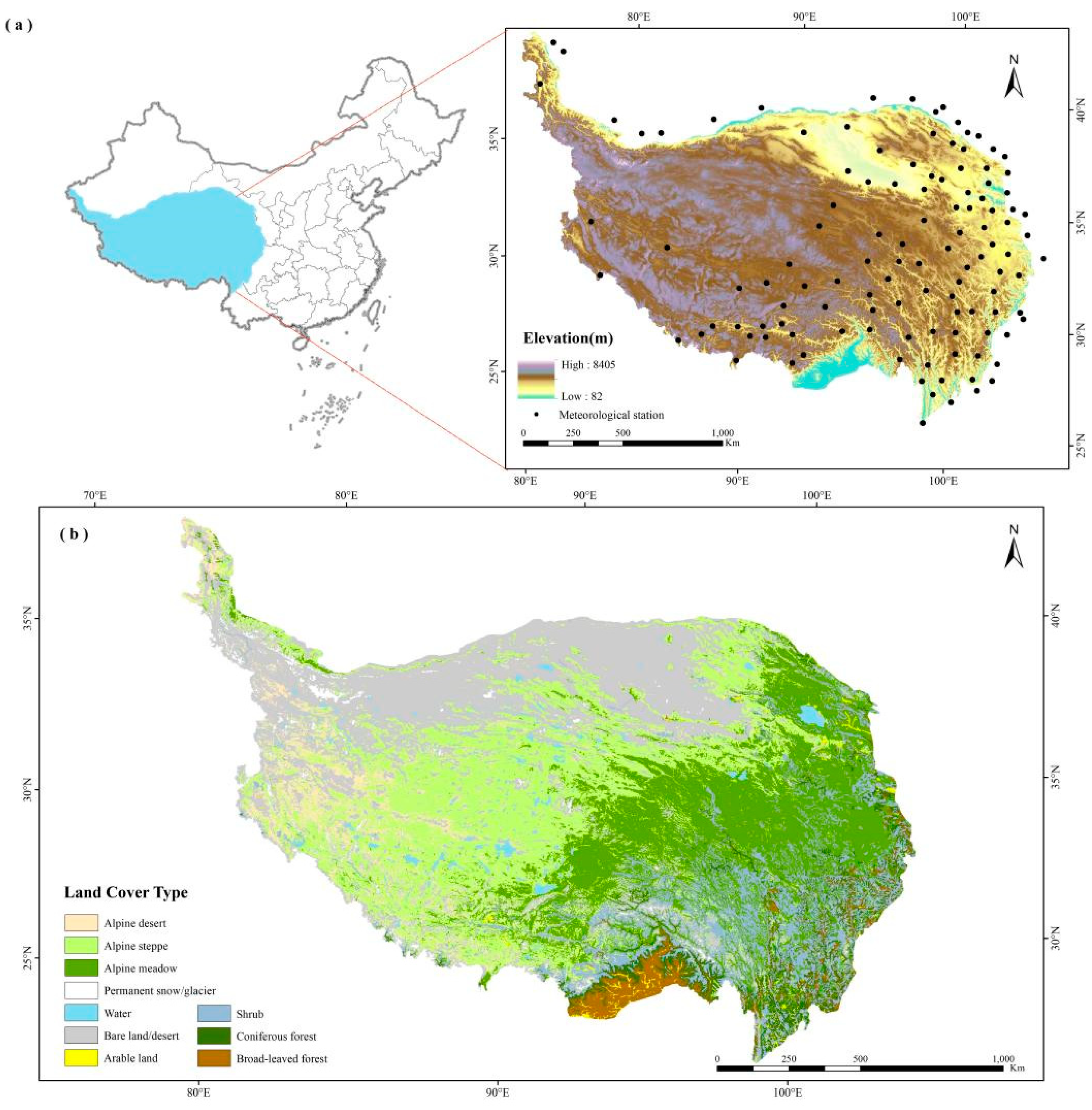
2.1. Study Area

The Tibetan Plateau (TP) is situated in southwestern China (73°–105° E, 26°–40° N), spanning an expansive area of approximately 2.57 × 10⁶ km² across six provinces which include Tibet, Qinghai, Gansu, Xinjiang, Sichuan, and Yunnan (Figure 1a). The TP is the physical geographical unit with the highest average elevation worldwide (exceeding 4000 m). The internal topography of the TP is complex and diverse, with a series of large mountains and topographic drops. The terrain displays a gradual descent from the northwest towards the southeast. The complex nature of the subsurface contributes to the unique climatic characteristics of the TP, with intense solar radiation, low air temperature, obvious diurnal temperature differences, and significant seasonal precipitation [32]. Depending on its unique natural conditions, the TP has nurtured rich and diverse ecosystems, and plays an important role as a barrier to the ecological security of China and eastern region of Asia [38].

2.2. Data

The study employed the NDVI dataset derived from NASA’s MOD13A2 product (https://ladsweb.nascom.nasa.gov/search/ (accessed on 8 March 2023)) for the period spanning 2001 to 2020, featuring a spatial resolution of 1 km. The product presents a composite representation of the optimal pixels over a 16-day interval. Notably, in contrast to daily products, it significantly diminishes the influence of disturbances like clouds and atmospheric factors [39]. Daily climate data (including daily maximum air temperature, daily minimum air temperature, and daily precipitation) was obtained from the Chinese National Meteorological Center (NMC) (http://data.cma.cn/ (accessed on 13 March 2023)). Considering the continuity of data at the stations, the study selected a total of 117 meteorological stations with continuous records between 2001 and 2020 on the TP and its surrounding areas. The LST product (https://espa.cr.usgs.gov/ (accessed on 8 March 2023)) is a three-level data product with a spatial resolution of 1 km from MODIS sensors and includes both daytime and nighttime LST data. Null values in LST data were filled by calculating the mean value of neighboring pixels. The height difference data (DEM data) was acquired from the Resource and Environmental Science Data Platform (RESDC) (https://www.resdc.cn/ (accessed on 10 March 2023)). Vegetation type data was acquired from the Science Data Bank (https://www.scidb.cn/doi/10.11922/sciencedb.398 (accessed on 12 March 2023)). The vegetation was segmented based on major vegetation types, including steppes, meadows, shrubs, cultivated vegetation, and forest (Figure 1b). The study focuses on discussing four vegetation types on the TP, namely steppes, meadows, shrubs and forests.

2.3. Methods

2.3.1. Preprocessing of NDVI Data

Prior to extracting vegetation phenology, we screened the pixels to eliminate the influence of snow lines, evergreen vegetation, sparse vegetation, and bare soil, retaining only valid pixels (Figure 2). The valid pixels had to meet the following criteria: (1) The average NDVI from April to September had to exceed 0.10, (2) the annual maximum NDVI had to be greater than 0.15 [40,41], (3) the annual maximum NDVI had to occur between July and September, and (4) the average NDVI in winter had to be less than 0.4 [42,43].

2.3.2. Dynamic Threshold Method

In the study, we selected the dynamic threshold method in TIMESAT software version 3.3 to extract the vegetation phenology of the Qinghai-Tibet Plateau. The dynamic threshold method can effectively reduce the uncertainty in the phenology extraction process [44]. In comparison to other extraction methods, it is more straightforward to implement and has a wider range of applicability, rendering it particularly well-suited to regions such as the TP, where there are considerable variations in hydrothermal conditions. The principle of the method is to define the amplitude of NDVI by determining the maximum and minimum values of NDVI in the current year (Figure 3). When NDVI reaches or falls below a fixed percentage of the maximum amplitude, it is determined as the beginning and end of the vegetation growing season [5]. The method is applied in the form of a dynamic ratio, and the threshold is adjusted according to the actual amplitude of NDVI for each pixel in the current year, thus avoiding differences in NDVI values between different vegetation types. The calculation formula is as follows:

$${NDVI}_{ratio}={\displaystyle \frac{NDVI-{NDVI}_{min}}{{NDVI}_{max}-{NDVI}_{min}}}$$

NDVI represents the reconstructed NDVI value; NDVI_max indicates the highest NDVI value observed annually; NDVI_min indicates the lowest NDVI value observed annually. Following the review of previous studies, we set the dynamic threshold of autumn phenology to 0.6. When NDVI_ratio is less than 0.6, the horizontal coordinate value at this point indicates the end date of the vegetation growing season.

2.3.3. Theil-Sen Trend Analysis and Mann-Kendall (MK) Test

Based on 20 years of EOS data extracted by the dynamic threshold method, the change trend of autumn phenology across the TP during the period of 2001–2020 was analyzed on a pixel-by-pixel basis using the Theil-Sen trend method. This trend analysis method is capable of effectively circumventing the potential influence of outliers on the results, and it does not have high requirements on the form of data distribution [45]. Based on time series analysis, it involves calculating the slope between each pair of year data for the same pixel and arranging all the calculated slopes in order from largest to smallest. The slope in the middle order is the final calculation result. The analytical formula is as follows:

$$\beta =Median\left({\displaystyle \frac{x_j-x_i}{j-i}}\right),2001\le i,j\le 2020$$

where, x_i represents the vegetation phenology data of year i, x_j represents the vegetation phenology data of year j, and β represents the long-term trend in vegetation phenology changes. Positive and negative values of β indicate delayed and advanced trends in vegetation phenology, respectively.

The Mann-Kendall (MK) test is a non-parametric method for detecting trends based on ranks. In this paper, we utilized the MK test to assess the significance of changing trends in autumn phenology time series. The test does not assume any specific distribution pattern for the samples. The parameter Z was employed for the purpose of statistically testing the significance of the changing trend, with significance levels of 0.1, 0.05, and 0.01.

2.3.4. Rescaled Range Analysis

In this study, the Hurst index, calculated by the R/S analysis method, was employed for analyzing the persistence of the change trend. The Hurst index has a value range of 0 < H < 1. If the H value exceeds 0.5, it suggests that the future trend will continue to follow its previous trend, with the value closer to 1 indicating a stronger consistency of the trend. If the H value is equal to 0.5, it means that the future change of the time series is uncertain. If the H value is lower than 0.5, it indicates that the future trend will go against the past trend and become anti-consistent. Given the time series {EOS (t)}, t = 1, 2, …, n, for any positive integer m ≥ 1, the following statistical metrics are defined sequentially [46].

• Mean sequence: $\overline{EOS\left(m\right)}={\displaystyle \frac{1}{m}}\sum _{t=1}^{m}EOS\left(m\right)m=\mathrm{1,2},\cdots ,n$
• Cumulative deviation: $X(t,m)=\sum _{t=1}^m\left(EOS\left(m\right)-\overline{EOS\left(m\right)}\right)1\le t\le m$
• Extreme deviation: $R\left(m\right)=maxEOS\left(t,m\right)-minEOS\left(t,m\right)m=\mathrm{1,2},\cdots ,n$
• Standard deviation: $S\left(m\right)={\left[{\displaystyle \frac{1}{m}}\sum _{t=1}^m{\left(EOS\left(t\right)-EOS\left(m\right)\right)}^2\right]}^{{\displaystyle \frac{1}{2}}}$

2.3.5. Partial Correlation Analysis

We used partial correlation analysis to explore the relationship between autumn phenology and climate in the TP. The partial correlation analysis method has the advantage of eliminating the confounding effects of one and more covariates [47]. Assuming that there are m variables X₁, X₂, …, X_m, the sample partial correlation coefficient of order k (k $\le$ m − 2) for any two variables X_i and X_j is computed as follows:

$$r_{{ij.l}_1{l}_{2\dots }{l}_m}={\displaystyle \frac{r_{{ij.l}_1{l}_{2\dots }{l}_{m-1}}-r_{{il}_m.l_1{l}_{2\dots }{l}_{m-1}}{r}_{{jl}_m.l_1{l}_{2\dots }{l}_{m-1}}}{\sqrt{(1-{r_{{il}_m.l_1{l}_{2\dots }{l}_{m-1}}}^2)(1-{r_{{jl}_m.l_1{l}_{2\dots }{l}_{m-1}}}^2)}}}$$

The significance test of partial correlation coefficient is conducted by t-test, and the calculation formula is described as:

$$t={\displaystyle \frac{r\sqrt{n-q-2}}{\sqrt{1-r^2}}}$$

where $r$ denotes the partial correlation coefficient, $n$ is the total number of years, and $q$ is the order (the number of independent variables).

3. Results

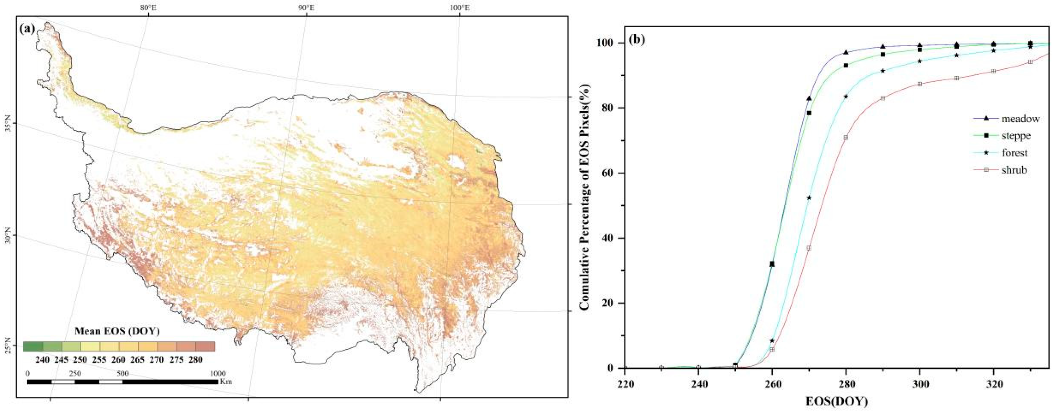
3.1. Spatial Patterns of Autumn Phenology

Over the past 20 years, the mean EOS occurred between DOY 240 and 280 (August to October) in 91.56% of the study area. The EOS only ended earlier than DOY 240 in 0.06% of the area. Spatially, the EOS in the southwestern and southeastern marginal regions of the TP generally occurred after DOY 280, significantly later than that in other regions, while the EOS in the central and northeastern regions ended significantly earlier (Figure 4a). The EOS for different vegetation types on the TP exhibited significant variations (Figure 4b). The meadows had a mean EOS of DOY 264, while the steppes had a slightly later mean EOS of DOY 265. On the other hand, the shrubs typically reached their EOS around DOY 272, while the forests had a later mean EOS of DOY 279. In general, the EOS for the meadows ranged from DOY 250 to 270, while the EOS for the steppes varied between DOY 250 and 275. The EOS for the shrubs was mainly within the range of DOY 255 to 280, while forests exhibited a broader range between DOY 255 and 285.

3.2. Spatiotemporal Variation of Autumn Phenology

In the TP, the EOS showed a marginally delayed trend at a rate of 0.017 days/year over the past 20 years. Spatially, a delayed trend in EOS was evenly distributed throughout the region, accounting for 56.18% of the entire area (Figure 5). Among them, approximately 6.16% were statistically significant (p < 0.05). Additionally, 43.82% of the region exhibited an advancement trend in EOS, with only 4.13% being statistically significant (p < 0.05). Earlier trends of EOS were primarily distributed in the southwest edge and northeast of the TP. Consistent with the overall trend observed within the study area, all vegetation types displayed a delaying trend in EOS. However, the rate of delay exhibited subtle variations with relatively modest distinctions among the different vegetation types. The shrubs exhibited an approximate delay rate of 0.04 days/year, while the meadows experienced a delay rate of approximately 0.03 days/year. Similarly, both the steppes and forests displayed a delay rate of approximately 0.02 days/year for their respective EOS.

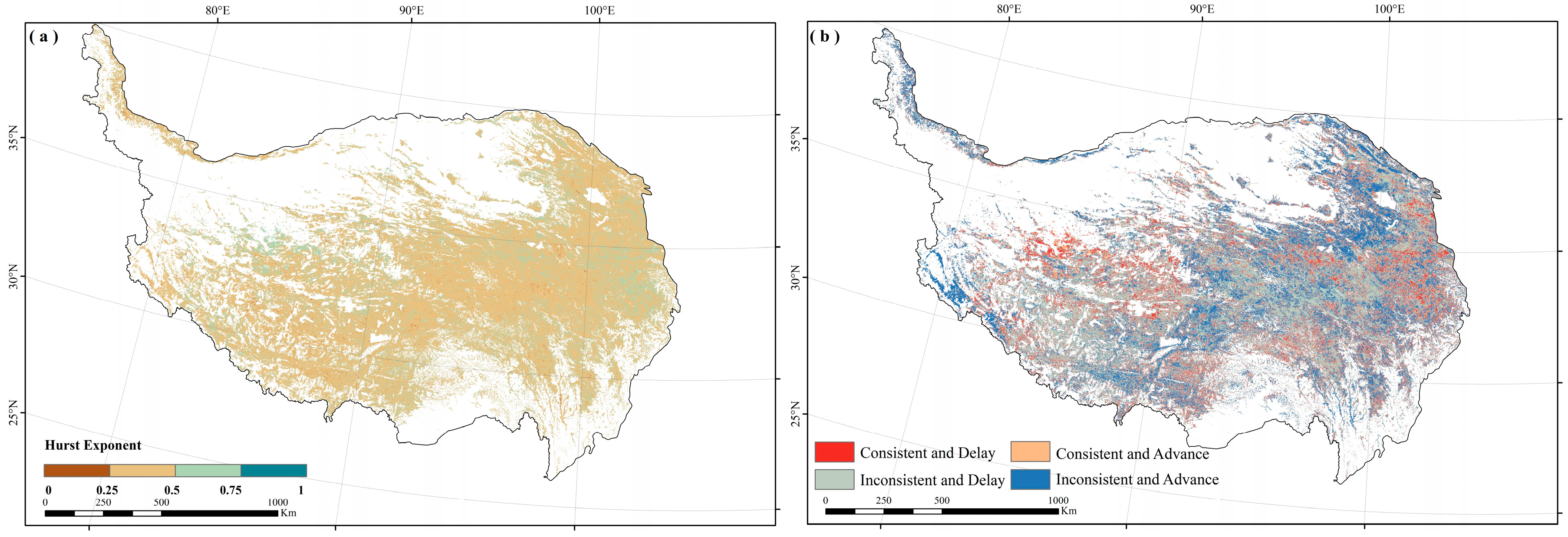
3.3. Consistency of Autumn Phenology Trends

The results of estimating the Hurst index based on R/S analysis showed that the mean value of the Hurst index across the Tibetan Plateau was 0.45. Specifically, up to 79.19% of the areas with a Hurst index of less than 0.5 were spread across the TP, while the remaining areas with a Hurst index above 0.5 were more scattered, with a larger area distributed along the borders of Qinghai, Gansu, and Sichuan provinces, as well as in the northern part of the Xizang Autonomous Region (Figure 6a). Combined with the results of the trend analysis, 11.99% and 8.89% of the areas were characterized by consistent delay and advance in future trends, respectively, while 46.96% and 32.16% of the areas were characterized by inconsistent delay and advance, respectively. In the future change trends, the region showing an advanced trend was predominantly found in the west of Qinghai Lake and the southeastern part of Xizang Autonomous Region, while the distribution of other regions was scattered. The delayed trend areas were primarily located in the central part of Xizang Autonomous Region and near the borders of Xizang, Qinghai and Sichuan provinces (Figure 6b).

3.4. Relationship between Altitude and Autumn Phenology

During the period from 2001 to 2020, the EOS of the TP had a clear elevation dependence, with a general trend of EOS advancement with increasing altitude (Figure 7a). Throughout the study area, the EOS advanced by 0.99 days for every 300 m increase in altitude (p < 0.05). From the perspective of vegetation zoning, the relationships between EOS and altitude for the four vegetation types were consistent with the region as a whole, with all showing a significant negative correlation (Figure 7b–e). For the four vegetation types, forests showed the fastest rate of change with altitude, with an EOS advance of 1.59 days/300 m (p < 0.001), followed by meadows with an EOS advance of 1.29 days/300 m (p < 0.001), and shrubs (p < 0.05) and steppes (p < 0.01) showed a similar rate with an EOS advance of 0.86 days/300 m. Among them, shrubs and steppes turned at about 4000 m above sea level, which was manifested by the fact that the EOS below 4000 m showed an advance with altitude, while above 4000 m the EOS mainly fluctuated between DOY 270 and 280, showing a weaker postponement trend.

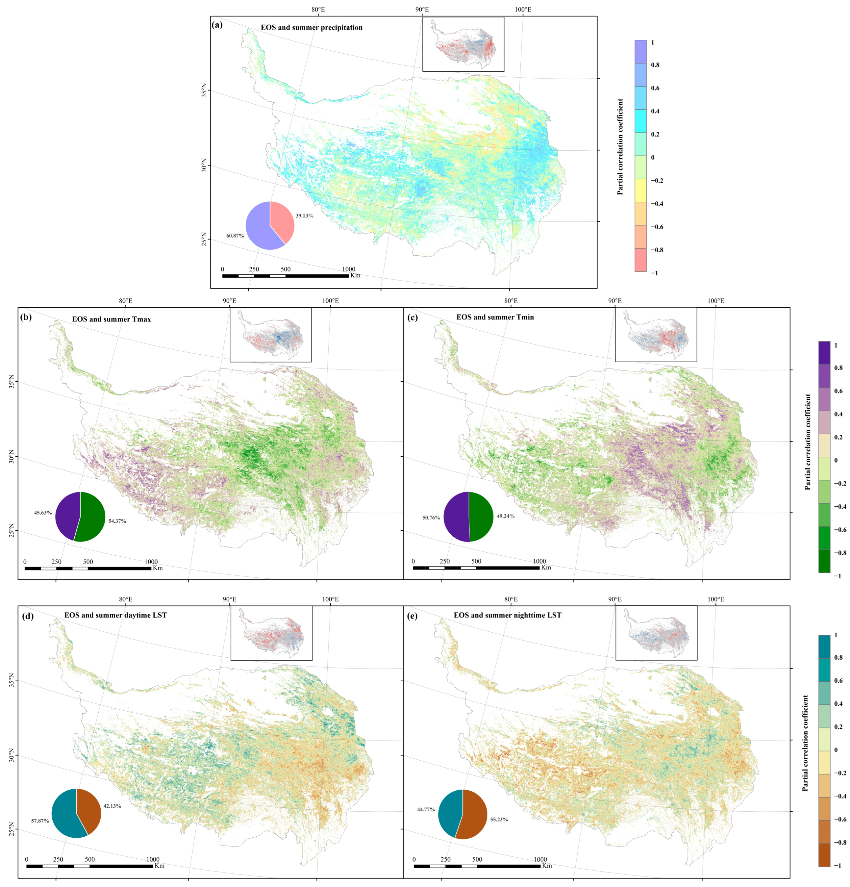
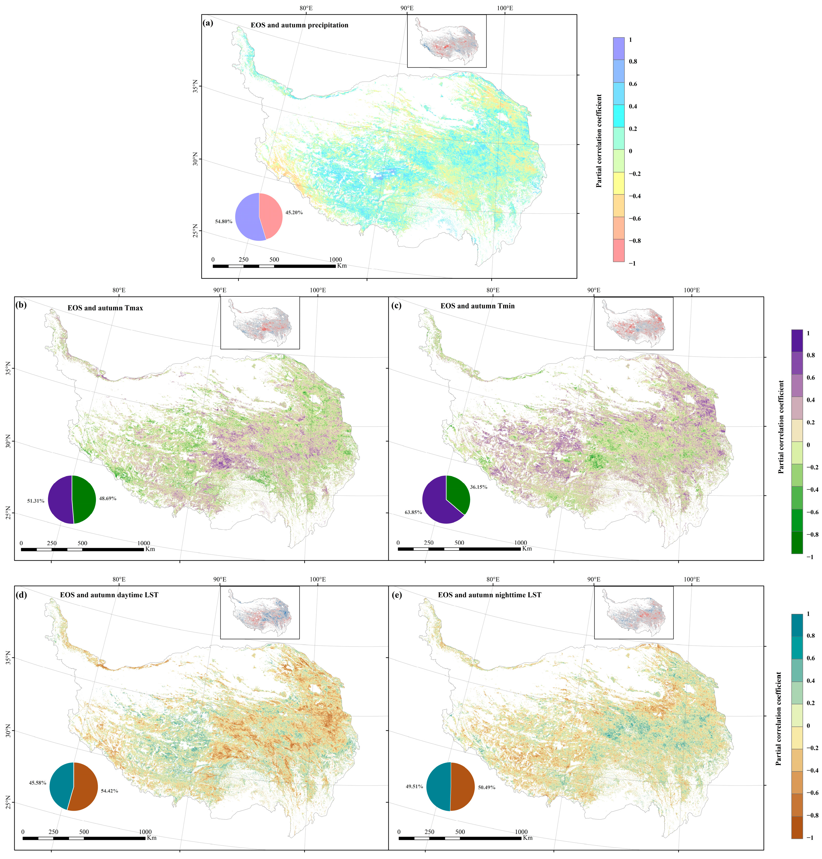
3.5. Response of Autumn Phenology to Climatic Factors

The relationship between autumn phenology in the TP and climatic factors in summer and autumn was investigated based on Pearson’s partial correlation coefficients. For the summer climate factors, 60.87% of the area was positively correlated with summer precipitation (Figure 8a), with a significant positive correlation (p < 0.05) for only 11.64% of the entire area, mainly in the eastern part of the Tibetan Plateau (southeastern Qinghai Province and northwestern Sichuan Province) and the west. The significant negative correlation (p < 0.05) accounted for 6.45%, which was concentrated in Qinghai Province. Regarding the impact of air temperatures (Figure 8b,c), T_max and T_min showed clear diurnal asymmetric effects on the EOS. Approximately 45.63% of the region experienced a positive influence from the summer T_max on the EOS. Among these, 6.97% of the entire area exhibited a significant impact (p < 0.05), primarily concentrated in the southwestern part of the plateau. While the area with significant negative correlation was relatively large (9.69%), distributed in the east and west sides of the TP. Compared with T_max, the spatial distribution pattern of positive and negative effects of T_min on EOS was basically opposite. Within the entire region, T_min had an equal share of positive and negative effects on the EOS. Among these, the area with a significant positive impact constituted 8.48%, predominantly located in the central part of the plateau. The area with a significant negative impact accounted for 7.32%, dispersed on either side of the plateau. Consistent with air temperature, daytime and nighttime LST also had significant diurnal asymmetric effects on the EOS (Figure 8d,e). Specifically, in nearly 60% of the area, summer daytime LST exerted a positive impact on the EOS, with the significantly affected areas accounting for 11.41%, primarily concentrated in the northeastern and western regions of the TP. However, regions with a significantly negative impact only constituted half of the areas exhibiting significant positive effects (5.69%), and their distribution was scattered. Less than 45% of the region showed a positive impact of nighttime LST on the EOS, with only 5.37% exhibiting significant effects, while the significant impact in areas with a negative influence covered 8.50%.

For the autumn climate factors, the results showed that in the majority of pixels, precipitation (54.80%) and T_min (63.85%) had a positive impact on the EOS (Figure 9a,c), while daytime LST (54.42%) had a negative impact (Figure 9d). Both the positive and negative impact of T_max and nighttime LST accounted for approximately 50% each, with neither having dominant influence (Figure 9b,e). The significant positive impact (8.11%) of precipitation on EOS was mainly observed in the western part of the TP, while the significant negative impact (6.19%) was concentrated in the southwestern margin. Regarding T_max, the areas exhibiting a significant positive impact (7.52%) on the EOS were concentrated in the central part of the TP, while the distribution of significant negative impact (6.12%) was scattered widely. In contrast to T_max, areas with a significant positive impact (12.85%) on the EOS due to T_min were distributed in the eastern and northeastern parts of the TP, while regions with a significant negative impact (3.61%) were scattered sporadically in the central area. As for daytime LST, the areas with a positive impact (7.36%) were concentrated in the central area of Xizang, while regions with a significant negative impact (11.66%) were in the eastern and southern parts of Qinghai Province. As for nighttime LST, most of the significant positive impact areas (7.10%) were distributed in the eastern part of the plateau, while the negative impact areas (7.13%) were primarily located in the central region of Qinghai Province, with sporadic distribution in the other regions.

Among the summer climate factors (Figure 10a), the factors that played a dominant role in EOS change were LST (43.75%), air temperature (32.91%), and precipitation (23.34%) in descending order, with the area dominated by LST having a large distribution on both the eastern and western sides of the plateau, the area dominated by air temperature concentrated in the central part, and the area dominated by precipitation concentrated in the eastern part. The order of leading climate factors in autumn was consistent with that in summer (Figure 10b), but the spatial distribution pattern was different. The dominant region of LST (43.82%) was concentrated in the eastern part of the plateau, the dominant region of air temperature (36.41%) was mainly concentrated in the western and northeastern part of the plateau, while the dominant region of precipitation (19.77%) had no obvious spatial distribution pattern.

4. Discussion

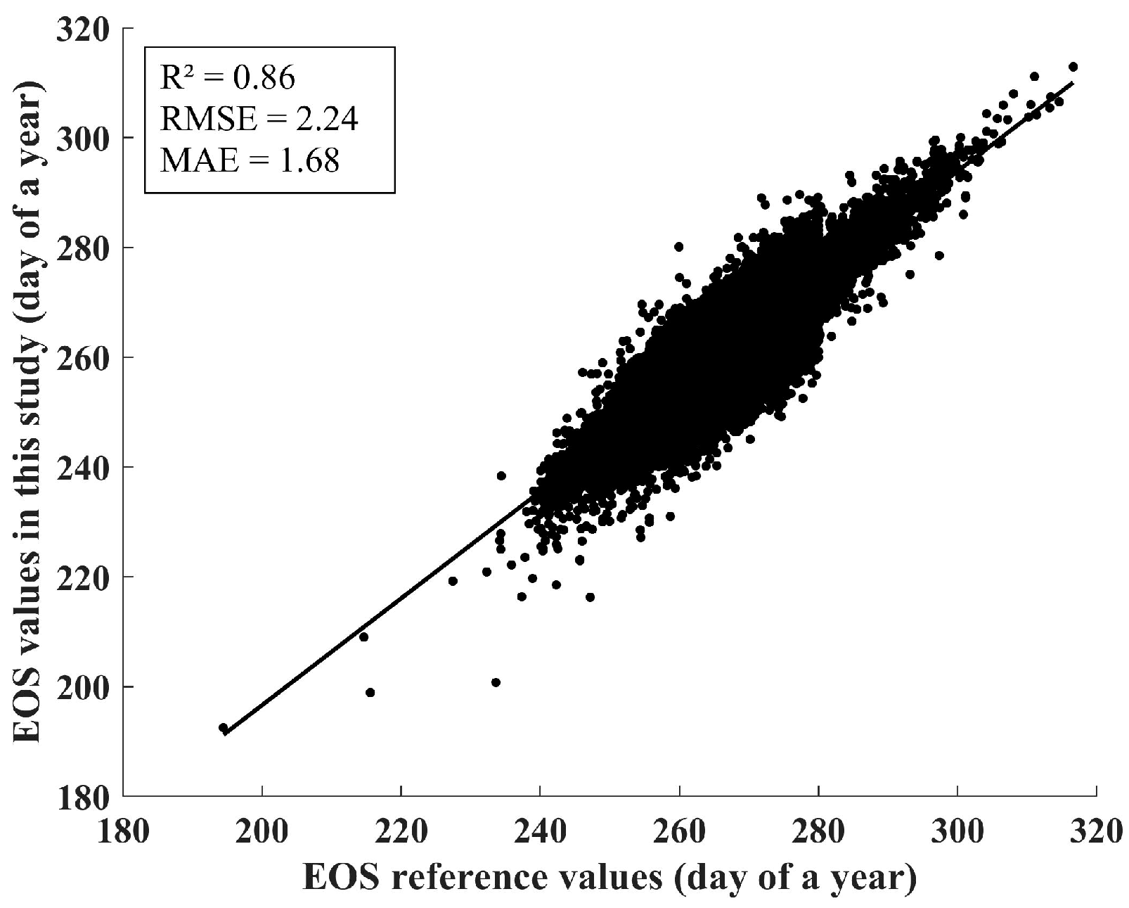
4.1. Indirect Validation of the EOS

In this study, the EOS was calculated from remotely sensed data based on the definition of vegetation phenology. Although actual site-based phenology data for direct validation was unavailable, the reliability of the results was ensured by indirect verification with an appropriate phenology product (Zu’s product published by Big Earth Data for Three Poles (http://poles.tpdc.ac.cn/zh-hans/) (accessed on 10 August 2024)). The evaluation metrics included the correlation coefficient (R²), root mean square error (RMSE), and mean absolute error (MAE). As illustrated in Figure 11, the EOS exhibited an R² of 0.86, an RMSE of 2.24 days, and an MAE of 1.68 days, indicating that the accuracy of the data is guaranteed to some extent.

4.2. Temporal and Spatial Pattern of Autumn Phenology

Autumn phenology was calculated using the dynamic threshold method based on 20 years (2001–2020) of NDVI data provided by NASA in the study. Over the entire study area, the results showed that the EOS occurred between DOY 240 and 280, with the average EOS of DOY 266, which was generally in accord with previous studies [39,48]. Early EOS was observed in meadows and steppes, while it was delayed in forests and shrubs. It is primarily affected by the natural conditions of the vegetation types. Meadows and steppes are distributed in the western region of the plateau, with less precipitation. In contrast, forests and shrubs are situated in the southwestern part of the plateau, with abundant water and heat conditions that favor vegetation growth. Over the past 20 years, we found that the EOS demonstrated a delay trend on the TP. Furthermore, numerous previous studies provided evidence that EOS was consistently delayed due to global warming [49,50]. However, the absolute change rate of EOS was far below that of SOS. Additionally, the delayed rate of EOS (0.017 days/year) in the TP was much smaller than that in the Yellow River Basin (0.37 days/year) [49] and Guangdong-Hong Kong-Macao Greater Bay Area (0.52 days/year) [51]. The discrepancies might be highly attributable to different areas. Due to high-intensity human activity, the Yellow River Basin and the Greater Bay experienced more intense climate change, resulting in more profound changes in the region’s vegetation phenology. For four vegetation types, a delaying trend in EOS was observed, and their tendency difference could be negligible.

4.3. Response of Autumn Vegetation to Climate Change

Our study found a positive correlation between precipitation (summer and autumn) and EOS in most areas of the Tibetan Plateau, implying that an increase in precipitation would contribute to a later EOS. This result was consistent with most studies on autumn phenology [50,52]. In general, plants experience increased water loss in higher temperature environments, particularly during the summer season. This can result in decreased water content in plant tissues, which can impact their normal metabolism [53,54]. In some cases, the loss may even exceed the amount of water absorbed. However, an increase in precipitation can help alleviate this water stress, ultimately delaying the EOS [55,56]. Contrary to prior research findings, rising summer T_max appeared to extend the EOS in semi-arid regions. This novel occurrence may arise from the inclination of the region’s aridity to limit the availability of moisture, whereby elevating T_max in summer causes the vegetation to experience water pressure by accelerated evaporation. Vegetation may adapt to environmental stress by regulating its physiological processes and reducing its growth rate to better utilize limited water resources, potentially delaying the EOS. In the TP, EOS was positively related to summer T_min in pixels that passed significance at the level of 0.05, suggesting that elevated summer T_min caused a delay in EOS. With the rise of summer T_min, leaf respiration naturally intensifies, causing an accelerated depletion of plant carbohydrates. This occurrence may trigger a compensatory mechanism to replenish the lost organic matter through the rebound effect of photosynthesis on the following day [57,58]. This rebound effect aids plants in utilizing carbon sources more efficiently to sustain growth and survival. This process carries significant implications for the carbon balance and adaptation strategies of plants, especially in the context of global warming, where increased nighttime temperatures may become more prevalent. This rebound effect has been extensively studied and reported, and it has been shown that this compensatory effect induced by nocturnal warming produces more organic matter than is consumed by increased respiration [59,60,61]. It explains why warmer T_min could delay the EOS. It is widely recognized that LST is a critical factor in the growth of vegetation and a vast body of research has confirmed that it affects the physiological functioning of the vegetative root system primarily by influencing soil properties. Warmer LST contributes to higher soil temperature, particularly in the top layer. This elevated soil environment stimulates growth and activity in the root systems of plants, enabling them to absorb essential water and nutrients required for photosynthesis and development. Additionally, warmer autumn air temperatures could delay the EOS. Leaf senescence involves a decrease in chlorophyll content [62]. In autumn, higher air temperatures can slow down chlorophyll degradation [19,63,64] resulting from the interaction between photosynthetic enzymes and chlorophyll. In warmer conditions, photosynthetic enzyme activity increases, allowing plants to better maintain leaf function and pigmentation [65]. This physiological regulation allows for longer periods of photosynthesis, maximizing light energy use for growth and metabolism while delaying leaf senescence. Additionally, this regulation may positively impact a plant’s ecosystem stability and adaptability. Warmer LST could advance the EOS. This may be due to two reasons. On the one hand, under the influence of soil moisture stress, an increase in autumn LST causes a simultaneous increase in soil moisture evaporation and plant transpiration, which means that the soil moisture conditions required for vegetation growth cannot be maintained [66]. On the other hand, under the influence of high respiration rates, the consumption of organic matter by the vegetation is accelerated and leaves senesce prematurely.

4.4. Analysis of Dominant Factors Affecting Autumn Phenology

Overall, our results demonstrate that the percentage of area with LST as the predominant climatic factor was over 40% in both summer and autumn. In the TP region, characterized by its high altitude and harsh environmental conditions, vegetation exhibits adaptive strategies to cope with extreme factors such as low temperatures, aridity, and strong winds. A prevalent survival strategy employed by plants in this challenging environment is to shorten their height, sometimes even growing close to the ground [67]. Consequently, certain components of the TP’s vegetation tend to exhibit a low stature, particularly herbaceous species [68]. Land surface temperatures exhibit more pronounced fluctuations compared to atmospheric temperatures. Vegetation located near the land surface may demonstrate heightened sensitivity to changes in LST due to the plant roots’ ability to rapidly perceive variations in LST [66]. LST primarily affects soil nutrient absorption and transformation in plant growth by altering soil temperature [69]. Specifically, the activity of microorganisms and enzymes in the soil is crucial for nutrient transformation in plants. An increase in LST can influence the activity of microorganisms and enzymes in the soil. Generally, higher temperatures contribute to increased enzyme activity, promoting the decomposition of organic matter and nutrient release, thus providing plants with more nutrients for absorption. Additionally, nutrients in the soil are typically present in a dissolved state [70], and the increase in soil temperature aids in enhancing the solubility of nutrients [71]. Consequently, the roots of plants can more readily absorb nutrients from the soil. Moreover, the warm soil temperature can affect the flow of soil moisture, thereby influencing nutrient transport and distribution. The three vegetation types, forest, meadow, and shrub were consistent across the entire region, with the highest percentage of pixel area dominated by LST. In the autumn climate, the proportion of pixel areas in steppes dominated by LST was comparable to those dominated by air temperature, while the proportion dominated by precipitation was the largest among the four vegetation types (

Table 2. The proportion of pixels dominated by autumn climatic factors in each vegetation type (%).

Vegetation Type	Tmax	Tmin	Precipitation	Daytime LST	Nighttime LST
forest	12.10	22.55	20.72	25.62	19.01
meadow	16.02	18.88	16.66	27.78	20.66
shrub	14.60	19.38	17.86	28.36	19.79
steppe	14.93	24.08	22.77	20.60	17.62

). This observation may be attributed to the fact that the steppes of the TP are inherently located in a semi-arid region. Unlike other vegetation ecosystems with relatively abundant water resources, where vegetation may show greater adaptability to temperature fluctuations, water availability is a more critical factor limiting vegetation growth in the steppes [24,72]. Among the pixels dominated by LST, there were more pixels influenced by daytime LST. The finding can be ascribed to the substantial impact of daytime LST on evaporation rate and enzyme activity compared to nighttime LST. An increase in LST during the day can intensify the rate of evaporation, leading to reduced soil moisture [66]. This, in turn, exerts pressure on the water supply for plants and substantially influences EOS.

The study is limited in scope as it only examines vegetation phenology in the twenty-first century. Although it does illustrate the current trend in vegetation phenology changes, it lacks a comprehensive analysis of phenological characteristics of vegetation on the TP and does not facilitate the examination of vegetation phenology changes in response to climate fluctuations. Therefore, to obtain more comprehensive and precise findings, future research should consider extending the time frame.

5. Conclusions

This study analyzed the spatial-temporal variation characteristics in autumn vegetation phenology across the TP from 2001 to 2020. The results demonstrated that EOS generally occurred between DOY 240 and 280 throughout the entire region, exhibiting an advance from the edge to the middle. The EOS in the whole region displayed a marginal tendency towards delay, with an average rate of 0.017 days/year. Among all vegetation, shrubs showed the most pronounced delay, with a rate of 0.04 days/year. Subsequently, we investigated the impact of climate change on EOS through partial correlation analysis and identified the primary factor influencing the EOS. The EOS was delayed with increased summer and autumn precipitation. The increase in summer T_max led to the advancement of EOS, while the increase in summer T_min and autumn air temperatures caused its delay. The increase in summer daytime LST led to the delay of EOS, while the increase in summer nighttime LST and autumn daytime LST caused its advance. There were diurnal asymmetric effects of both LST and air temperatures on EOS. Based on the dominant factor analysis, LST was identified as the primary factor affecting EOS in both summer and autumn climate factors.

References

1. IPCC. Climate Change 2022: Mitigation of Climate Change. Contribution of Working Group III to the Sixth Assessment Report of the Intergovernmental Panel on Climate Change; IPCC: Geneva, Switzerland, 2022. [Google Scholar]
2. United Nations Environment Programme. Emissions Gap Report 2023: Broken Record: Temperatures Hit New Highs, Yet World Fails to Cut Emissions (Again); United Nations Environment Programme: Nairobi, Kenya, 2023. [Google Scholar]
3. Zhai, P.M.; Yu, R.; Zhou, B.Q.; Chen, Y.; Guo, J.; Lu, Y. Research Progress in Impact of 1.5 °C Global Warming on Global and Regional Scales. Adv. Clim. Chang. Res. 2022, 13, 465–472. [Google Scholar] [CrossRef]
4. Piao, S.; Liu, Q.; Chen, A.; Janssens, I.A.; Fu, Y.; Dai, J.; Liu, L.; Lian, X.; Shen, M.; Zhu, X. Plant phenology and global climate change: Current progresses and challenges. Global Chang. Biol. 2019, 25, 1922–1940. [Google Scholar] [CrossRef] [PubMed]
5. Gao, X.; Zhao, D.S. Impacts of climate change on vegetation phenology over the Great Lakes Region of Central Asia from 1982 to 2014. Sci. Total Environ. 2022, 845, 157227. [Google Scholar] [CrossRef]
6. Wang, Z.; Fu, B.; Wu, X.; Li, Y.; Feng, Y.; Wang, S.; Wei, F.; Zhang, L. Vegetation resilience does not increase consistently with greening in China’s Loess Plateau. Commun. Earth Environ. 2023, 4, 336. [Google Scholar] [CrossRef]
7. Xu, X.; Riley, W.J.; Koven, C.D.; Jia, G.; Zhang, X. Earlier leaf-out warms air in the north. Nat. Clim. Chang. 2020, 10, 370–375. [Google Scholar] [CrossRef]
8. Richardson, A.D.; Keenan, T.F.; Migliavacca, M.; Ryu, Y.; Sonnentaf, O.; Toomey, M. Climate change, phenology, and phenological control of vegetation feedbacks to the climate system. Agric. For. Meteorol. 2013, 169, 156–173. [Google Scholar] [CrossRef]
9. Wang, M.; Luo, Y.; Zhang, Z.; Xie, Q.; Wu, X.; Ma, X. Recent advances in remote sensing of vegetation phenology: Retrieval algorithm and validation strategy. Natl. Remote Sens. Bull. 2022, 26, 431–455. [Google Scholar] [CrossRef]
10. Peng, D.; Zhang, X.; Zhang, B.; Liu, L.; Liu, X.; Huete, A.; Huang, W.; Wang, S.; Luo, S.; Zhang, X.; et al. Scaling effects on spring phenology detections from MODIS data at multiple spatial resolutions over the contiguous United States. ISPRS J. Photogramm. Remote Sens. 2017, 132, 185–198. [Google Scholar] [CrossRef]
11. Xi, X.; Zhao, G.X. Chlorophyll content in winter wheat: Inversion and monitoring based on UAV multi-spectral remote sensing. Chin. Agric. Sci. Bull. 2020, 36, 119–126. [Google Scholar] [CrossRef]
12. Julien, Y.; Sobrino, J.A. Global land surface phenology trends from GIMMS database. Int. J. Remote Sens. 2009, 30, 3495–3513. [Google Scholar] [CrossRef]
13. Wu, L.Z.; Ma, X.F.; Dou, X.; Zhu, J.T.; Zhao, C.Y. Impacts of climate change on vegetation phenology and net primary productivity in arid Central Asia. Sci. Total Environ. 2021, 796, 149055. [Google Scholar] [CrossRef]
14. Doussoulin-Guzmán, M.A.; Pérez-Porras, F.J.; Triviño-Tarradas, P.; Rios-Mesa, A.; Garcia-Ferrer, P.; Mesas-Carrascosa, F.J. Grassland Phenology Response to Climate Conditions in Biobio, Chile from 2001 to 2020. Remote Sens. 2022, 14, 475. [Google Scholar] [CrossRef]
15. Bradley, A.V.; Gerard, F.F.; Barbier, N.; Weedon, G.P.; Anderson, L.O.; Huntingford, C.; Aragao, L.; Zelazowski, P.; Arai, E. Relationships between phenology, radiation and precipitation in the Amazon region. Glob. Chang. Biol. 2011, 17, 2245–2260. [Google Scholar] [CrossRef]
16. Duarte, L.; Teodoro, A.C.; Monteiro, A.T.; Cunha, M.; Goncalves, H. QPhenoMetrics: An open source software application to assess vegetation phenology metrics. Comput. Electron. Agric. 2018, 148, 82–94. [Google Scholar] [CrossRef]
17. Gao, B.C.; Li, R.R. Quantitative improvement in the estimates of NDVI values from remotely sensed data by correcting thin cirrus scattering effects. Remote Sens. Environ. 2000, 74, 494–502. [Google Scholar] [CrossRef]
18. Skakun, S.; Franch, B.; Vermote, E.; Roger, J.C.; Becker-Reshef, I.; Justice, C.; Kussul, N. Early season large-area winter crop mapping using MODIS NDVI data, growing degree days information and a Gaussian mixture model. Remote Sens. Environ. 2017, 195, 244–258. [Google Scholar] [CrossRef]
19. Liu, Q.; Fu, Y.H.; Zhu, Z.; Liu, Y.; Liu, Z.; Huang, M.; Janssens, I.A.; Piao, S. Delayed autumn phenology in the Northern Hemisphere is related to change in both climate and spring phenology. Glob. Chang. Biol. 2016, 22, 3702–3711. [Google Scholar] [CrossRef] [PubMed]
20. Garonna, I.; de Jong, R.; Schaepman, M.E. Variability and evolution of global land surface phenology over the past three decades (1982–2012). Glob. Chang. Biol. 2016, 22, 1456–1468. [Google Scholar] [CrossRef] [PubMed]
21. Linderholm, H.W. Growing season changes in the last century. Agric. For. Meteorol. 2006, 137, 1–14. [Google Scholar] [CrossRef]
22. Piao, S.; Fang, J.; Zhou, L.; Ciais, P.; Zhu, B. Variations in satellite-derived phenology in China’s temperate vegetation. Glob. Chang. Biol. 2006, 12, 672–685. [Google Scholar] [CrossRef]
23. Yun, J.; Jeong, S.J.; Ho, C.H.; Park, C.E.; Park, H.; Kin, J. Influence of winter precipitation on spring phenology in boreal forests. Glob. Chang. Biol. 2018, 24, 5176–5187. [Google Scholar] [CrossRef] [PubMed]
24. Ren, S.L.; Li, Y.T.; Peichl, M. Diverse effects of climate at different times on grassland phenology in mid-latitude of the Northern Hemisphere. Ecol. Indic. 2020, 113, 106260. [Google Scholar] [CrossRef]
25. Li, P.; Peng, C.; Wang, M.; Luo, Y.; Li, M.; Zhangg, K.; Zhan, D.; Zhu, Q. dynamics of vegetation autumn phenology and its response to multiple environmental factors from 1982 to 2012 on Qinghai-Tibetan Plateau in China. Sci. Total Environ. 2018, 637, 855–864. [Google Scholar] [CrossRef] [PubMed]
26. Chen, X.; Li, B.; Li, Q.; Li, J.; Abdulla, S. Spatio-temporal pattern and changes of evapotranspiration in arid Central Asia and Xinjiang of China. J. Arid. Land 2012, 4, 105–112. [Google Scholar] [CrossRef]
27. Jiang, W.; Niu, Z.; Wang, L.; Yao, R.; Gui, X.; Xiang, F.; Ji, Y. Impacts of Drought and Climatic Factors on Vegetation Dynamics in the Yellow River Basin and Yangtze River Basin, China. Remote Sens. 2022, 14, 930. [Google Scholar] [CrossRef]
28. Gou, Y.; Jin, Z.; Kou, P.; Tao, Y.; Xu, Q.; Zhu, W.; Tian, H. Mechanisms of climate change impacts on vegetation and prediction of changes on the Loess Plateau, China. Environ. Earth Sci. 2024, 83, 234. [Google Scholar] [CrossRef]
29. Chen, X.; An, S.; Inouye, D.W.; Schwartz, M.D. Temperature and snowfall trigger alpine vegetation green-up on the world’s roof. Glob. Chang. Biol. 2015, 21, 3635–3646. [Google Scholar] [CrossRef] [PubMed]
30. Sun, H.; Chen, Y.; Xiong, J.; Ye, C.; Yong, Z.; Wang, Y.; He, D.; Xu, S. Relationships between climate change, phenology, edaphic factors, and net primary productivity across the Tibetan Plateau. Int. J. Appl. Earth Obs. Geoinf. 2022, 107, 102708. [Google Scholar] [CrossRef]
31. Fu, B.J.; Ouyang, Z.Y.; Shi, P. Current Condition and Protection Strategies of Qinghai-Tibet Plateau Ecological Security Barrier. Bull. Chin. Acad. Sci. 2021, 36, 1298–1306. [Google Scholar] [CrossRef]
32. Zhang, Q.; Kong, D.D.; Shi, P.J.; Singh, V.P.; Sun, P. Vegetation phenology on the Qinghai-Tibetan Plateau and its response to climate change (1982–2013). Agric. For. Meteorol. 2018, 248, 408–417. [Google Scholar] [CrossRef]
33. Mo, S.G.; Zhang, B.P.; Cheng, W.M. Major Environmental Effects of the Tibetan Plateau. Prog. Geogr. 2004, 23, 88–96. [Google Scholar] [CrossRef]
34. Yao, T.D.; Zhu, L.P. The response of environmental changes on Tibetan Plateau to global changes and adaptation strategy. Adv. Earth Sci. 2006, 21, 459–464. [Google Scholar] [CrossRef]
35. Piao, S.L.; Cui, M.D.; Chen, A.P.; Wang, X.; Ciais, P.; Liu, J.; Tang, Y. Altitude and temperature dependence of change in the spring vegetation green-up date from 1982 to 2006 in the Qinghai-Xizang Plateau. Agric. For. Meteorol. 2011, 151, 1599–1608. [Google Scholar] [CrossRef]
36. Chen, D.; Xu, B.; Yao, T.; Guo, Z.; Cui, P.; Chen, F.; Zhang, T. Assessment of past, present and future environmental changes on the Tibetan Plateau. Chin. Sci. Bull. 2015, 60, 3025–3035. [Google Scholar] [CrossRef]
37. Ding, Y.H.; Ren, G.Y.; Shi, G.Y. National assessment report of climate change (l): Climate change in China and its future trend. Adv. Clim. Chang. Res. 2006, 2, 3–8. [Google Scholar]
38. Wang, X.Y.; Wu, C.Y.; Peng, D.L.; Gonsamo, A.; Liu, Z.J. Snow cover phenology affects alpine vegetation growth dynamics on the Tibetan Plateau: Satellite observed evidence, impacts of different biomes, and climate drivers. Agric. For. Meteorol. 2018, 256–257, 61–74. [Google Scholar] [CrossRef]
39. Zu, J.; Zhang, Y.; Huang, K.; Liu, Y.; Chen, N.; Cong, N. Biological and climate factors co-regulated spatial-temporal dynamics of vegetation autumn phenology on the Tibetan Plateau. Int. J. Appl. Earth Obs. Geoinf. 2018, 69, 198–205. [Google Scholar] [CrossRef]
40. Chen, X.; Wang, L. Progress in remote sensing phenological research. Prog. Geog. 2009, 28, 33–40. [Google Scholar] [CrossRef]
41. Shao, Z.; Zhou, W.; Li, F.; Zhou, X.; Yang, F. Spatiotemporal variation of vegetation phenophase and its response to climate change in Micang Mountains from 2003 to 2018. Acta Ecol. Sin. 2021, 41, 3701–3712. [Google Scholar] [CrossRef]
42. Shen, M.; Tang, Y.; Jin, C.; Zhu, X.; Zheng, Y. Influences of temperature and precipitation before the growingseason on spring phenology in grasslands of the central and eastern Qinghai-Tibetan Plateau. Agric. For. Meteorol. 2011, 151, 1711–1722. [Google Scholar] [CrossRef]
43. Ding, M.; Zhang, Y.; Sun, X.; Liu, L.; Wang, Z. Spatiotemporal variation in alpine grassland phenology in the Qinghai-Tibetan Plateau from 1999 to 2009. Chin. Sci. Bull. 2012, 57, 3185–3194. [Google Scholar] [CrossRef]
44. Jonsson, P.; Eklundh, L. Seasonality extraction by function fitting to time-series of satellite sensor data. IEEE Trans. Geosci. Remote Sens. 2002, 40, 1824–1832. [Google Scholar] [CrossRef]
45. Su, Y.; Zhang, F.; Liu, B. Response of forest vegetation phenology to climate change in Xiaoxing’an Mountains of northeastern China. J. Beijing For. Univ. 2023, 45, 34–47. [Google Scholar] [CrossRef]
46. Ying, H.; Zhang, H.Y.; Zhao, J.J.; Shan, Y.; Zhang, Z.; Guo, X.; Rihan, W.; Deng, G. Effects of spring and summer extreme climate events on the autumn phenology of different vegetation types of Inner Mongolia, China, from 1982 to 2015. Ecol. Indic. 2020, 111, 105974. [Google Scholar] [CrossRef]
47. Piao, S.; Liu, Z.; Wang, T.; Peng, S.; Ciais, P.; Huang, M.; Ahlstrom, A.; Burkhart, J.F.; Chevallier, F.; Janssens, I.A.; et al. Weakening temperature control on the interannual variations of spring carbon uptake across northern lands. Nat. Clim. Chang. 2017, 7, 359–363. [Google Scholar] [CrossRef]
48. Liu, M.; Li, Y.; He, B.; Zhao, W. Spatiotemporal Dynamics of Grassland Phenology and Sensitivity to Extreme Precipitation in Autumn in Qinghai-Tibetan Plateau. Res. Soil Water Conserv. 2023, 30, 353–363. [Google Scholar] [CrossRef]
49. Yuan, M.; Zhao, L.; Lin, A.; Li, Q.; She, D.; Qu, S. How do climatic and non-climatic factors contribute to the dynamics of vegetation autumn phenology in the Yellow River Basin, China? Ecol. Indic. 2020, 112, 106112. [Google Scholar] [CrossRef]
50. Ma, R.; Shen, X.; Zhang, J.; Xia, C.; Liu, Y.; Wu, L.; Wang, Y.; Jiang, M.; Lu, X. Variation of vegetation autumn phenology and its climatic drivers in temperate grasslands of China. Int. J. Appl. Earth Obs. Geoinf. 2022, 114, 103064. [Google Scholar] [CrossRef]
51. Yang, X.; Fan, F. Land surface phenology and its response to climate change in the Guangdong-Hong Kong-Macao Greater Bay Area during 2001–2020. Ecol. Indic. 2023, 154, 10728. [Google Scholar] [CrossRef]
52. Xie, B.N.; Qin, Z.F.; Wang, Y.; Chang, Q.R. Monitoring vegetation phenology and their response to climate change on Chinese Loess Plateau based on remote sensing. Trans. Chin. Soc. Agric. Eng. 2015, 31, 153–160. [Google Scholar] [CrossRef]
53. Jiao, K.; Gao, J.; Wu, S. Climatic determinants impacting the distribution of greenness in China: Regional differentiation and spatial variability. Int. J. Biometeorol. 2019, 63, 523–533. [Google Scholar] [CrossRef]
54. Shen, X.; Jiang, M.; Lu, X.; Liu, X.; Liu, B.; Zhang, J.; Wang, X.; Tong, S.; Lei, G.; Wang, S.; et al. Aboveground biomass and its spatial distribution pattern of herbaceous marsh vegetation in China. Sci. China Earth Sci. 2021, 64, 1115–1125. [Google Scholar] [CrossRef]
55. Fang, W.; Huang, S.; Huang, Q.; Huang, G.; Wang, H.; Leng, G.; Wang, L. Probabilistic assessment of remote sensing-based terrestrial vegetation vulnerability to drought stress of the Loess Plateau in China. Remote Sens Environ. 2019, 232, 111290. [Google Scholar] [CrossRef]
56. Yue, P.; Zhang, Q.; Ren, X.; Ren, X.; Yang, Z.; Li, H.; Yang, Y. Environmental and biophysical effects of evapotranspiration in semiarid grassland and maize cropland ecosystems over the summer monsoon transition zone of China. Agric. Water Manag. 2022, 264, 107462. [Google Scholar] [CrossRef]
57. Shen, X.; Liu, B.; Li, G.; Zhou, D. lmpact of Climate Change on Temperate and Alpine Grasslands in China during 1982–2006. Adv. Meteorol. 2015, 10, 180614. [Google Scholar] [CrossRef]
58. Wang, Y.; Shen, X.; Jiang, M.; Lu, X. Vegetation Change and Its Response to Climate Change between 2000 and 2016 in Marshes of the Songnen Plain, Northeast China. Sustainability 2020, 12, 3569. [Google Scholar] [CrossRef]
59. Peng, S.; Piao, S.; Ciais, P.; Myneni, R.B.; Chen, A.; Chevallier, F.; Dolman, J.A.; Janssens, I.A.; Peñuelas, J.; Zhang, G.; et al. Asymmetric effects of daytime and night-time warming on Northern Hemisphere vegetation. Nature 2013, 501, 88–92. [Google Scholar] [CrossRef]
60. Xia, H.; Li, A.; Feng, G. The Effects of Asymmetric Diurnal Warming on Vegetation Growth of the Tibetan Plateau over the Past Three Decades. Sustainability 2018, 10, 1103. [Google Scholar] [CrossRef]
61. Shen, X.; Liu, Y.; Zhang, J.; Wang, Y.; Ma, R.; Liu, B.; Lu, X.; Jiang, M. Asymmetric impacts of diurnal warming on vegetation carbon sequestration of marshes in the Qinghai Tibet Plateau. Glob. Biogeochem. Cycles 2022, 36, e2022GB007396. [Google Scholar] [CrossRef]
62. Huang, P.; Li, Z.; Guo, H. New Advances in the regulation of leaf Senescence by classical and peptide hormones. Front. Plant Sci. 2022, 13, 923136. [Google Scholar] [CrossRef] [PubMed]
63. Thomas, P.; Janave, M.T. Effect of temperature on chlorophyllase activity, chlorophyll degradation and carotenoids of Cavendish bananas during ripening. Int. J. Food Sci. Technol. 1992, 27, 57–63. [Google Scholar] [CrossRef]
64. Shi, C.; Sun, G.; Zhang, H.; Xiao, B.; Ze, B.; Zhang, N.; Wu, N. Effects of warming on chlorophyll degradation and carbohydrate accumulation of Alpine herbaceous species during plant senescence on the Tibetan Plateau. PLoS ONE 2014, 9, e107874. [Google Scholar] [CrossRef]
65. Moore, C.E.; Meacham-Hensold, K.; Lemonnier, P.; Slattery, R.A.; Benjamin, C.; Bernacchi, C.J.; Lawson, T.; Cavanagh, A.P. The effect of increasing temperature on crop photosynthesis: From enzymes to ecosystems. J. Exp. Bot. 2021, 72, 2822–2844. [Google Scholar] [CrossRef]
66. Li, X.; Guo, W.; Li, S.; Zhang, J.; Ni, X. The different impacts of the daytime and nighttime land surface temperatures on the alpine grassland phenology. Ecosphere 2021, 12, e03578. [Google Scholar] [CrossRef]
67. He, T.; Wu, M.X.; Jia, J.F. Research advances in morphology and anatomy of alpine plants growing in the Qinghai-Tibet Plateau and their adaptations to environment. Acta Ecol. Sin. 2007, 27, 2574–2583. [Google Scholar] [CrossRef]
68. Ernakovich, J.G.; Hopping, K.A.; Berdanier, A.B.; Simpson, R.T.; Kachergis, E.J.; Steltzer, H.; Wallenstein, M.D. Predicted responses of arctic and alpine ecosystems to altered seasonality under climate change. Glob. Chang. Biol. 2014, 20, 3256–3269. [Google Scholar] [CrossRef]
69. Onwuka, B.; Mang, B. Effects of soil temperature on some soil properties and plant growth. Adv. Plants Agric. Res. 2018, 8, 34–37. [Google Scholar] [CrossRef]
70. Reichardt, K.; Timm, L.C. How Plants Absorb Nutrients from the Soil. In Soil, Plant and Atmosphere; Springer Nature: Cham, Switzerland, 2020. [Google Scholar] [CrossRef]
71. Pregitzer, K.; King, J. Effects of Soil Temperature on Nutrient Uptake. In Nutrient Acquisition by Plants; BassiriRad, H., Ed.; Ecological Studies; Springer: Berlin/Heidelberg, Germany, 2005; Volume 181, pp. 277–310. [Google Scholar] [CrossRef]
72. Shen, X.; Liu, B.; Henderson, M.; Wang, L.; Wu, Z.; Wu, H.; Jiang, M.; Lu, X. Asymmetric effects of daytime and nighttime warming on spring phenology in the temperate grasslands of China. Agric. For. Meteorol. 2018, 259, 240–249. [Google Scholar] [CrossRef]
Figure 1. (a) The location and elevation of the TP within China; (b) the distribution of land cover types.
Forests 15 01476 g001
Figure 2. Valid areas in the TP.
Forests 15 01476 g002
Figure 3. Concept map for phenological parameter extraction.
Forests 15 01476 g003
Figure 4. (a) The spatial distribution of annual mean EOS; (b) the cumulative percentage of the EOS pixels for the four vegetation types.
Forests 15 01476 g004
Figure 5. Spatial distribution of EOS trend during 2001–2020. The picture in the lower left corner shows the significant level of the trend.
Forests 15 01476 g005
Figure 6. The spatial distribution of (a) the H values of the EOS; (b) the future trend of the EOS.
Forests 15 01476 g006
Figure 7. Relationship between EOS and altitude in (a) whole region (b) forest (c) meadow (d) shrub (e) steppe of the TP.
Forests 15 01476 g007
Figure 8. The spatial distribution pattern of partial correlation coefficient between EOS and summer climate factors across the TP from 2001 to 2020. The climate variable contains (a) precipitation, (b) Tmax, (c) Tmin, (d) daytime LST, (e) nighttime LST. The pictures in the higher right corner show the significant partial correlations, with the color blue representing negative partial correlations, and the color red representing positive partial correlations.
Forests 15 01476 g008
Figure 9. The spatial distribution pattern of partial correlation coefficient between EOS and autumn climate factors across the TP from 2001 to 2020. The pictures in the higher right corner show the significant partial correlations (the same as Figure 8).
Forests 15 01476 g009
Figure 10. Spatial distribution pattern of the dominant climatic factor on EOS (a) in summer and (b) in autumn based on the maximum partial correlation coefficient.
Forests 15 01476 g010
Figure 11. Comparison of the EOS results of the study with the EOS values of other phenological products.
Forests 15 01476 g011