Multi-Dimensional Landscape Connectivity Index for Prioritizing Forest Cover Change Scenarios: A Case Study of Southeast China

Abstract

Predicting forest cover change (FCC) and screening development scenarios are crucial for ecological resilience. However, quantitative evaluations of prioritizing forest change scenarios are limited. Here, we took five shared socio-economic pathways (SSPs) representing potential global changes, namely SSP1: sustainability, SSP2: middle of the road, SSP3: regional rivalry, SSP4: inequality, and SSP5: fossil-fueled development, which were constructed by integrated assessment and climate models. We modeled them with the patch-generating land use simulation (PLUS) and constructed a multi-dimensional landscape connectivity index (MLCI) employing forest landscape connectivity (FLC) indices to assess forest development in Fujian Province, Southeast China. The MLCI visualized by radar charts was based on five metrics, including forest patch size (class area (CA), number (patch density (PD), isolation (landscape division index (DIVISION), aggregation (mean nearest-neighbor index (ENN_MN), and connectance index, (CONNECT). The results indicate that FC will remain above 61.4% until 2030, with growth observed in SSP1 and SSP4. Particularly, FC in SSP4 substantially increased, converted from cropland (1140.809 km²) and grassland (645.741 km²). SSP4 has the largest MLCI values and demonstrates significant enhancements in forest landscape integrity, with CA, ENN_MN and CONNECT increasing greatly. Our study offers valuable approaches to and insights into forest protection and restoration.

1. Introduction

Forest cover (FC) is a vital component of terrestrial ecosystems and plays a crucial role in preserving biodiversity. However, the decline in FC may result in very far-reaching consequences for biodiversity that it makes a global concern [1,2]. Currently, the FC area in China keeps expanding, while the loss and reforestation of forest interior have caused the fragmentation of forests and the decline in forest landscape connectivity (FLC), negatively impacting the ecological environment of forests [3]. Specifically, during the period from the 6th (1999–2009) to the 9th national forest resource inventory (2014–2018), the FC area in China increased from 0.175 billion hm² to 0.220 billion hm², and the FC rate rose by 4.8%. Nevertheless, forest fragmentation has climbed from 0.383 to 0.393 over the past 20 years [4,5,6]. Additionally, it is of great significance to preserve FLC, which can mitigate forest cover change (FCC) driven by climate change and human activities, safeguard forest diversity, and regulate material and energy flows within forest ecosystems [7]. Therefore, FLC continues to be a significant focus of global research efforts aimed at addressing these complex challenges.

FLC has been used in diverse fields, such as habitat conservation, urban–rural environmental planning, and landscape regulation. In hundreds of FLC studies, landscape indices were mainly utilized to represent landscape pattern information and depict the landscape structure composition and spatial configuration of the study area quantitatively. Moreover, each index holds different ecological significances [8]. To explore FLC, Fragstats has been popularly implemented to calculate correlative landscape indices. Deng et al. [9], for example, utilized Fragstats to express the characteristics of land use/cover (LUC) patches in the Changsha–Zhuzhou–Xiangtan Metropolitan Area (Hunan Province, China). Similarly, Cai et al. [10] employed it to quantify the spatiotemporal characteristics of landscape change in the coastal areas of Fujian Province. Additionally, in northeastern New Mexico, Hayes et al. [11] utilized landscape indices to assess differences in fire responses among specific patches. Nevertheless, numerous studies merely analyze the characteristics of forest landscape using a single index, failing to comprehensively assess it, not to mention conducting comparisons of forest landscapes across different periods or regions, thereby disabling the ability to judge the quality of FLC. Therefore, there is an urgent need for comprehensive FLC indices that can reflect multi-dimensions effectively. However, assigning weights for each index becomes another great challenge. Presently, primary weighting methods include expert scoring [12], the analytic hierarchy process [13], and others. It has been found that these methods are relatively subjective and deeply influenced by human experience. On the other hand, methods like the regression analysis [14], the entropy weight method [15], and the principal components analysis [16] are entirely data-driven. What struck us was the multi-dimensional poverty index developed by Liu et al. [17], which not only demonstrated the independence of individual indices, but also provided a more objective reflection of regional differences and comparability than simple weighting methods. The calculation of the index in the study was grounded in the framework of vulnerability and sustainable livelihoods analysis established by the Department for International Development (DFID) [18]. After that, the study devised a comprehensive geo-identification indicator system for multi-dimensional poverty, including six dimensions (financial, human, natural, physical, and social capital, as well as environmental/contextual vulnerability). Based on this, they computed the comprehensive scores of each geographic unit to identify and categorize the types of poverty, leading to precisely identifying the multi-dimensional poverty counties. Inspired by this approach, we developed the multi-dimensional landscape connectivity index (MLCI) using radar maps, which provides an objective reflection of regional landscape connectivity while upholding the independence of individual indicators.

It is essential to predict future forest landscape patterns for effectively guiding forest conservation and restoration efforts. Thus, to achieve this, it is crucial to set up a range of scenario assumptions and examine potential changes across various paths. However, previous research predominantly neglected the significant impact of climate change on LUC, which impeded us from impartially evaluating what scenario is most in line with future development requirements, creating difficulties in optimizing LUC management policies. Notably, the shared socio-economic pathways (SSPs) were introduced by the Intergovernmental Panel on Climate Change (IPCC) [19] in its 5th assessment report on climate change, which include SSP1 (sustainability), SSP2 (middle of the road), SSP3 (regional rivalry), SSP4 (inequality), and SSP5 (fossil-fueled development), offering a framework for predicting future potential development scenarios [20]. These pathways serve as valuable references for researchers assessing the ecological environment’s impact [21]. Some scholars have already applied them to forecast population growth, GDP trends, urbanization patterns, and other critical aspects [22,23]. Moreover, the application of SSPs in predicting land use/cover change (LUCC) has emerged as a new frontier in current research [24,25]. Currently, many scholars employ simulation models that rely on the transition analysis strategy or the pattern analysis strategy, such as logistic cellular automata [26], cellular automata Markov [27], artificial neural network cellular automata [28], and future land use simulation (FLUS) models [29]. These models have constraints in elucidating the impact of driving factors on LUCC and are unable to simulate multiple LUC types at the patch level with spatiotemporal dynamics. Fortunately, the patch-generating land use simulation (PLUS) model, introduced by Liang et al. [30], overcomes these limitations and showcases significant advantages. Recently, several scholars have successfully integrated the SSPs and the PLUS model to predict LUCC, yielding valuable insights. For instance, Li et al. [31] utilized the PLUS model to project carbon emissions resulting from land use in the Chengdu-Chongqing economic zone under various SSPs. Similarly, Chen et al. [32] assessed the impact of ecosystem services in the Han River Basin within the framework of these scenarios. In this study, we adopted the SSPs and the PLUS model to forecast LUCC and FLC. Our objective is to deeply explore future LUCC trends and their potential impacts on FLC, thereby providing a more scientific and valuable reference for guiding future forest conservation and development efforts.

Currently, although numerous scholars employ SSPs, few quantitative methods are used in the comparison among scenarios, which restricts the practical value of scenario simulations. Additionally, scientific and systematic evaluation methods are still lacking in the optimization of scenarios. Therefore, this study established an MLCI analysis framework to measure the suitability of different scenarios for forest development, and Fujian Province was chosen as the study area. Fujian Province, situated in the southeast of China, has maintained the highest FC on the mainland for over 40 years [33]. However, the swift development in Fujian Province has resulted in remarkable dynamic changes in forest patches and the ecological environment being confronted with great pressure. In such a context, protecting the ecological environment has turned into a key factor for promoting high-quality economic development. Furthermore, we conformed to the unified plan of the national land planning outline (2016–2030) [34], using 2030 as the time node, and constructed the MLCI to examine the superior outcomes of prediction under the SSPs. The study aims to: (1) predict FCC in Fujian Province from 2020 to 2030; (2) analyze changes in FLC under different SSPs; and (3) determine the optimal scenario for the future development of FC in Fujian Province. This research seeks to address the ecological challenges stemming from the ongoing decline in FC and FLC in Fujian Province, promoting sustainable ecological environment development.

2. Materials and Methods

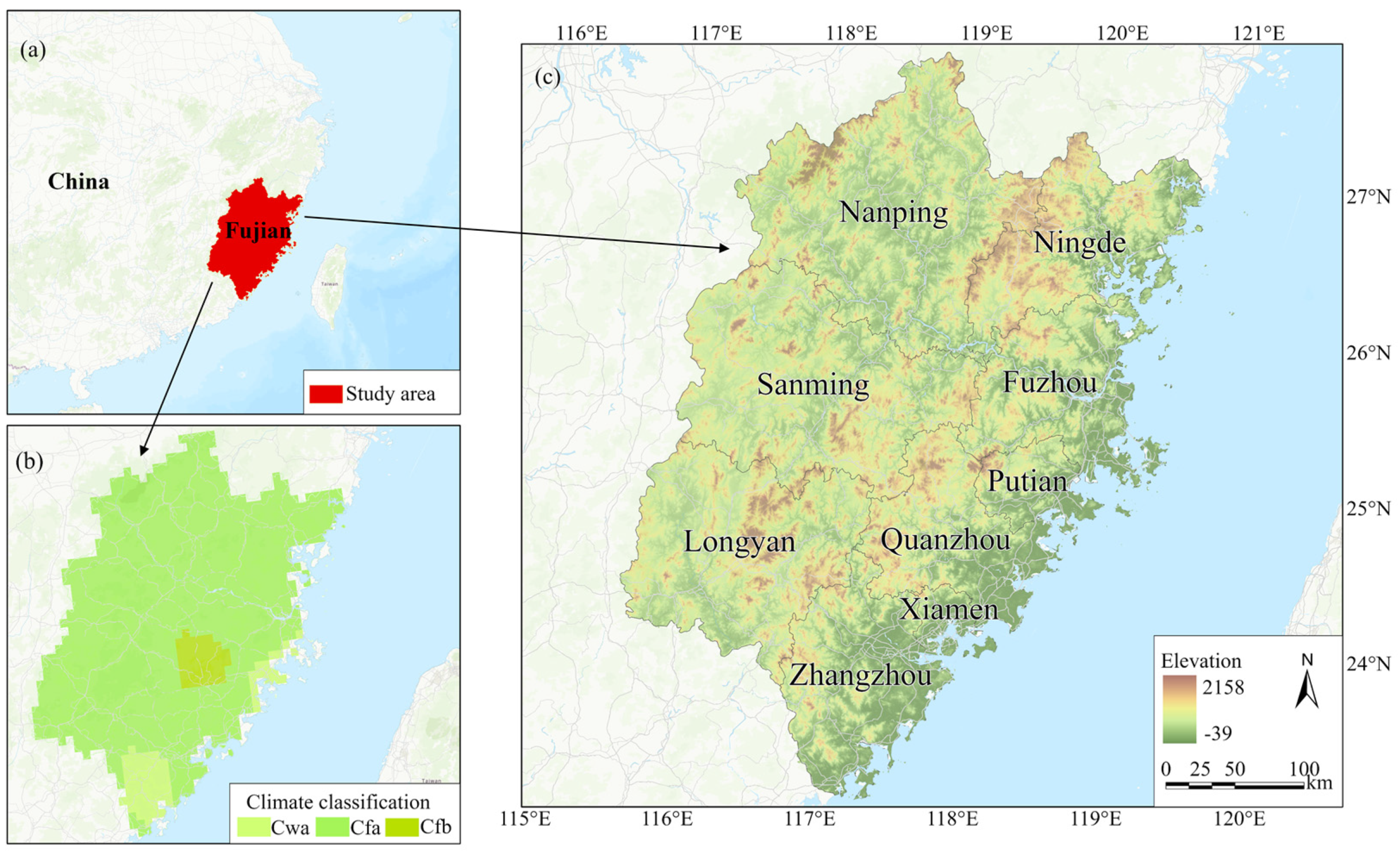
2.1. Study Area

The study area, Fujian Province (23°30′–28°22′ N, 115°50′–120°40′ E), covers approximately 124,000 km² and is characterized by a mountainous and hilly terrain, whose western and central areas are obliquely traversed by the Wuyi mountains and Daiyun mountains. The terrain ascends in the northwest and descends in the southeast (Figure 1). Fujian Province has a subtropical monsoon climate, with the annual temperature between 17 and 21 °C and precipitation ranging from 1000 to 2000 mm. Due to its unique natural conditions, the FC rate in Fujian Province is exceptionally high at 66.8%, boasting a variety of vegetation types [33]. These conditions supply vigorous safeguards for the ecological environment and biodiversity of Fujian Province.

2.2. Data Sources and Pre-Processing

The study utilized various datasets, including LUC, digital elevation model (DEM), climate, socio-economic data, and SSP database (

Table 1. Datasets used in this study.

Name	Resolution	Year	Sources
Land use/cover (LUC)	30 m	2000–2020	RESDC (https://www.resdc.cn, accessed on 9 July 2023)
Digital elevation model (DEM)	30 m	—	Geospatial data cloud (http://www.gscloud.cn, accessed on 9 July 2023)
Precipitation	1 km	2020	National Earth system science data center (http://www.geodata.cn, accessed on 12 July 2023)
Temperature
Population	1 km	2019	Resource environmental science data registry and publishing system (http://www.resdc.cn/DOI, accessed on 13 July 2023)
Population and gross domestic product (GDP)
Shared socio-economic pathways (SSPs) database	0.5°		NUIST disaster risk research team of Prof. Jiang T., graduate school of management (https://www.scidb.cn/en/detail?dataSetId=73c1ddbd79e54638bd0ca2a6bd48e3ff, accessed on 15 July 2023)

). LUC data were obtained from the resource and environment science and data center (RESDC) (https://www.resdc.cn, accessed on 9 July 2023), with a spatial resolution of 30 m from 2000 to 2020. The data were classified into six types: cropland, forest, grassland, water area, built-up land, and unused land. DEM data with a spatial resolution of 30 m, provided by the geospatial data cloud (http://www.gscloud.cn, accessed on 9 July 2023), were used to derive surface information, such as slope, aspect, and contour lines. The climate data for 2020, including monthly precipitation and temperature information with a spatial resolution of 1 km, were sourced from the national Earth system science data center (http://www.geodata.cn, accessed on 12 July 2023). The socio-economic data, including population and gross domestic product (GDP) with a spatial resolution of 1 km, were obtained from the resource environmental science data registry and publishing system (http://www.resdc.cn/DOI, accessed on 13 July 2023). The SSP database from 2020 to 2100 with a resolution of 0.5°, provided by the NUIST disaster risk research team, projected population and GDP data (https://www.scidb.cn/en/detail?dataSetId=73c1ddbd79e54638bd0ca2a6bd48e3ff, accessed on 15 July 2023) [24].

To investigate the impacts of FCC, ten factors were incorporated as driving forces in the PLUS model, including terrain (DEM, slope, and aspect), climate (monthly average temperature and precipitation), socio-economic indicators (population and GDP), and accessibility (distance to rivers, roads, and railways). We downscaled the climate, socio-economic, and SSPs data individually. For the climate and socio-economic data, we initially transformed them into point data; what followed was downscaled to a 30 × 30 m resolution by the inverse distance weighting method [35]. In terms of the population and GDP data from the SSPs database, it was assumed that the proportion of them remained constant over time. Initially, the grid was converted into points for interpolation based on the 2000 population and GDP data before downscaling the resulting dataset to 30 m. Next, we gathered the data from 2000 into 0.5° grids, and divided the 30 m count grid by the 0.5° count grid to derive the 30 m weight map. Subsequently, we substituted the grid cell with “1/30 m” whose denominator was 0 (indicating zero population at 0.5°). Ultimately, we multiplied the weight map with each 0.5° projection map to generate downscaled data [36]. These processing and analysis steps were conducted by the ArcGIS and PLUS models.

2.3. Methods

The research framework of this study consists of three modules: scenario design, LUC simulation, and MLCI construction (Figure 2). We employed ArcGIS 10.8 (made in Redlands, CA, USA) to calculate the dynamics degree of single land use, adopted the PLUS model developed by Liang et al. [30] to simulate scenarios, utilized ArcGIS 10.8 and GS+ 9.0 (made in Switzerland) to calculate the FLC indices, and employed Origin 2022 (made in Northampton, MA, USA) to visualize the MLCI. Eventually, we selected the optimal scenario to promote forest development and provide a scientific basis for preserving the ecological environment and biodiversity.

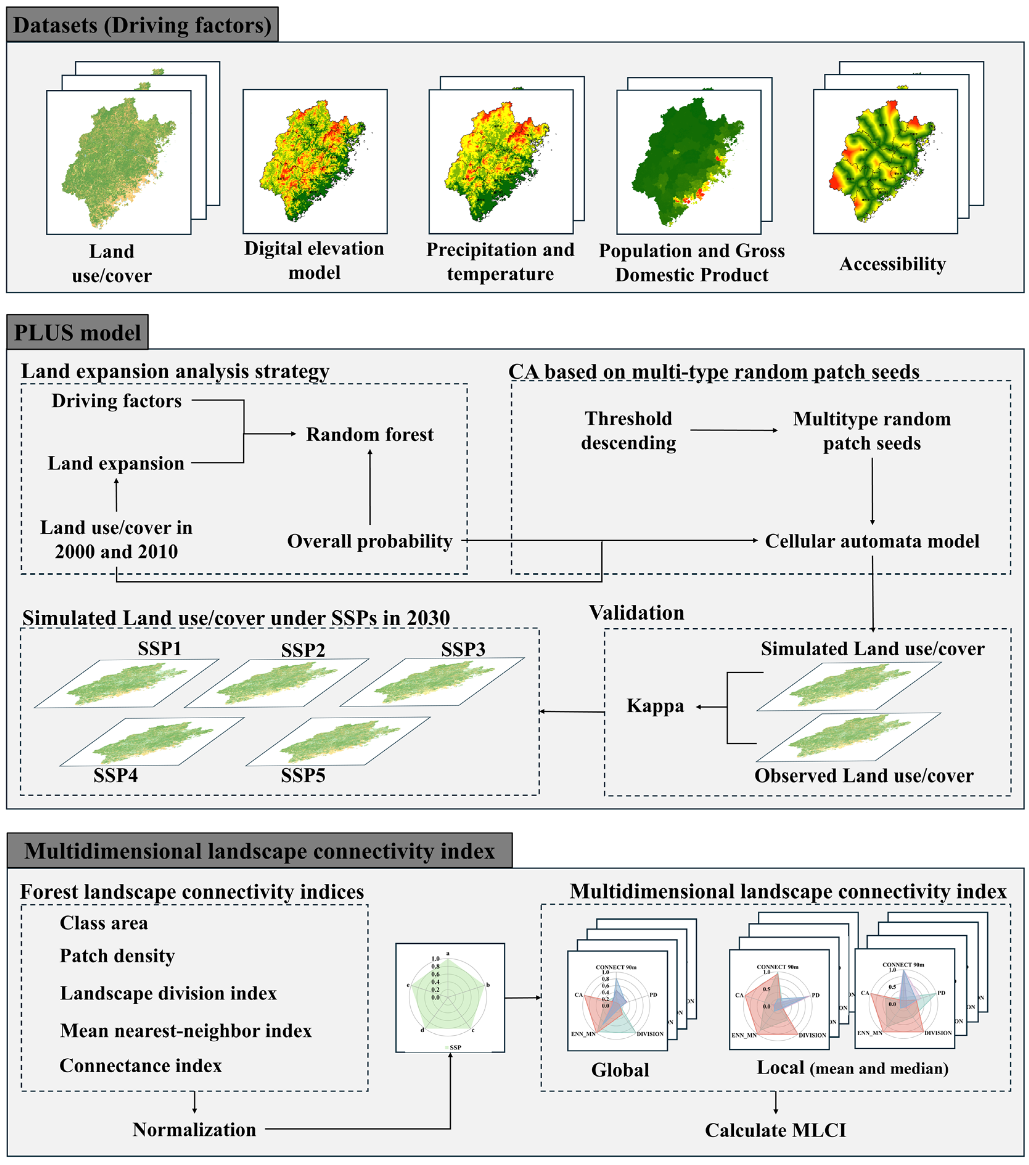
2.3.1. Dynamics Model of Land Use/Cover Changes

The dynamic degree of single land use (K) is frequently used to quantify the rate of land type area change. The absolute value of K reflects the intensity of LUCC, with the larger value indicating the more significant change. When the K value is above 0, it implies that the land expands, whereas when the value is below 0, it suggests that the area shrinks (Equation (1)) [37,38,39].

$$k={\displaystyle \frac{U_b-U_a}{U_a}}\times {\displaystyle \frac{1}{T}}\times 100\%$$

(1)

where U_a and U_b denote the areas of a specific LUC type at the beginning and end of the period, respectively. T represents the number of years between the two data periods.

2.3.2. Design of Multi-Scenarios

We selected five scenarios (SSP1, SSP2, SSP3, SSP4, and SSP5) to simulate FC and FLC in Fujian Province by 2030 (

Table 2. Conditions for the multi-scenarios.

Scenarios	Conditions
SSP1	Green and sustainable developments and strict regulation of LUCC.
SSP2	Continuing current social development and moderately regulating LUCC.
SSP3	Continuous regional competition and limited regulatory efforts for LUCC.
SSP4	Uneven development in different regions, well-regulated efforts for LUCC in middle-income and high-income countries, and poor development in low-income countries.
SSP5	Development relying mainly on fossil fuels and moderate supervision of LUCC.

) [20,23]. SSP1 emphasizes green and sustainable development as the principle, strictly regulating LUCC to prevent the worsening of environmental problems. In this scenario, the deforestation rate remains low, agricultural productivity improves, and there is an active pursuit of international cooperation to address climate change. SSP2 follows current societal development trends, with a moderate oversight of LUCC. The deforestation rate gradually decreases, agricultural productivity steadily improves, and global cooperation aims to combat climate change through semi-open approaches. SSP3 presents a worst-case scenario marked by ongoing regional competition and limited supervision of LUCC. Deforestation continues, agricultural productivity faces challenges, and global cooperation on climate change mitigation is severely delayed. SSP4 reflects uneven global development, with substantial advancements in LUCC regulations and agricultural productivity in middle-income and high-income countries, but inadequate progress in low-income countries. Furthermore, cooperation on climate change mitigation is primarily limited to well-developed nations. SSP5 relies on traditional fossil fuels for energy production, with moderate LUCC oversight. The deforestation rate shows a downward trend, agricultural productivity increases, and cooperation on climate change mitigation is postponed amidst extensive globalization efforts.

The conversion cost matrix serves as a vital tool for qualitatively describing SSPs, utilized to assess the feasibility of converting one land type to another [30]. Specific conversion cost matrices are developed for various scenario frameworks, as shown in

Table 3. The conversion the cost matrix in multi-scenarios.

	Cropland	Forest	Grassland	Water Area	Built-Up Land	Unused Land
	SSP1
Cropland	1	1	1	0	1	1
Forest	0	1	0	0	0	1
Grassland	0	1	1	0	0	1
Water area	0	0	0	1	1	1
Built-up land	1	1	1	0	1	1
Unused land	1	1	1	1	1	1
	SSP2
Cropland	1	0	0	0	1	1
Forest	0	1	0	0	1	1
Grassland	0	0	1	0	1	1
Water area	0	0	0	1	1	1
Built-up land	0	0	0	0	1	1
Unused land	1	1	1	1	1	1
	SSP3
Cropland	1	0	0	0	1	1
Forest	1	1	1	0	1	1
Grassland	1	0	1	0	1	1
Water area	0	0	0	1	0	1
Built-up land	1	0	0	0	1	1
Unused land	1	1	1	1	1	1
	SSP4
Cropland	1	1	1	0	1	1
Forest	0	1	1	0	0	1
Grassland	0	1	1	0	0	1
Water area	0	0	0	1	0	1
Built-up land	0	0	0	0	1	1
Unused land	1	1	1	1	1	1
	SSP5
Cropland	1	1	0	0	0	1
Forest	1	1	1	0	1	1
Grassland	1	0	1	0	1	1
Water area	0	0	0	1	0	1
Built-up land	1	0	0	0	1	1
Unused land	1	1	1	0	1	1

, where 1 indicates convertibility, while 0 signifies non-convertibility.

2.3.3. Simulation of Land Use/Cover Changes

The PLUS model consists of two main components: (1) a rule mining framework based on the land expansion analysis strategy (LEAS), and (2) a cellular automata (CA) model based on multitype random patch seeds (CARSs) [30]. The LEAS leverages two temporal datasets of LUC to identify changing units and analyze the expansion of each land type. Next, sub-datasets are created by randomly selecting sampling points and applying the labeling method to classify LUC types. Subsequently, the random forest (RF) algorithm [40] is applied to analyze the sub-datasets and driving factors to estimate the development probability of each category. In CARS, a multitype of the random patch seeding mechanism with threshold descent is employed under the constraint of development probability, along with the CA model to dynamically simulate future LUC patterns. Furthermore, the Markov chain model is widely employed to predict LUCC probability and demand [30]. In this study, the LUC area predicted by the Markov chain model was utilized as the input of land demand in CARS, and the change rate of these area was treated as the neighborhood weight. To evaluate the performance of the PLUS model, we employed three metrics: the Kappa coefficient, overall accuracy (OA), and figure of merit (FoM) [41,42,43]. Usually, the closer the Kappa coefficient and OA are to 1, the higher the accuracy of the model simulation. Although the Kappa coefficient has been widely used in previous studies to verify the simulation accuracy of the PLUS model, its reliability remains a subject of controversy [44]. Thus, we introduced the FoM coefficient to further verify the accuracy of PLUS. The coefficient assesses the model’s capability of predicting spatial distributions, serving as an effective tool to evaluate accuracy. Typically, its value less than 0.3, and the larger the value, the higher the simulation accuracy.

We inputted LUC data and ten driving factors into LEAS for 2000 and 2010. The factors included terrain (DEM, slope, and aspect), climate (monthly temperature and precipitation), socio-economic status (population and GDP), and accessibility (distance to rivers, roads, and railways). The RF algorithm was utilized to estimate the development probability of various LUC types. Subsequently, we employed the Markov chain model to predict the demand for LUC in 2020 and established a conversion cost matrix for LUCC in 2020 (Table 3). In the CARS model, to generate simulated LUC data for 2020, we used the development probability and predicted demand for LUC as input parameters. Finally, we assessed the accuracy of the simulated data for 2020 by the Kappa coefficient, OA, and FoM.

2.3.4. Selection and Calculation of Forest Landscape Connectivity Indices

To delineate the key characteristics of FLC, we adopted five FLC indices, including forest patch size (class area (CA), quantity (patch density (PD), isolation (landscape division index (DIVISION), aggregation (mean nearest-neighbor index (ENN_MN), and connectance index, (CONNECT) (

Table 4. List of forest landscape connectivity (FLC) indices used in the study.

Indices	Formulas	Description
Class area (CA)	${\sum }_{j=1}^n{a}_{ij}/\mathrm{10,000}$	CA represents the area of the patch type, measured in hectares (hm2), and is calculated by dividing the sum of patch type areas (m2) by 10,000. aij denotes the area of patch ij (m2).
Patch density (PD)	$n_i/A\times \mathrm{10,000}\times 100$	PD refers to the patch density, indicating the number of patches per 100 hectares. The higher the PD value, the higher the forest landscape fragmentation. ni signifies the value of patch i. A represents the total area of the landscape (m2).
Landscape division index (DIVISION)	$-{\sum }_{j=1}^n{(a_{ij}/A)}^2$	DIVISION represents the extent of dispersion of similar patches, serving as a metric to quantify the level of landscape fragmentation. A higher DIVISION value indicates greater landscape segregation. Value range: [0,1).
Mean nearest-neighbor index (ENN_MN)	${\displaystyle \frac{{\sum }_{j=1}^n{h}_{ij}}{n_i}}$	ENN_MN denotes the distance (m) between similar patches, judging if they are structurally connected. A larger value represents a larger distance between patches. hij is the nearest proximity of the patch, ij, to the same class patch.
Connectance index (CONNECT)	${\displaystyle \frac{{\sum }_{j\ne k}^n{C}_{ijk}}{\frac{n_i(n_i-1)}{2}}}\times 100$	CONNECT represents the number of nodes between specific patch classes divided by the number of potential nodes. The higher the patch connectivity, the greater the CONNECT value. Cijk denotes the connection between patches j and k linked to i within a critical distance.

) [45,46]. Landscape connectivity is defined as the measurement of continuity between structural units within the landscape, encompassing structural and functional aspects [47]. For the structural FLC, this study utilized the CA and PD indices to quantity the patch size and assess landscape fragmentation, respectively. For the functional FLC, we employed DIVISION and ENN_MN indices to evaluate the patch isolation and mean nearest-neighbor distance between patches, respectively. Additionally, the CONNECT index was utilized to provide a comprehensive assessment of landscape connectivity. To enhance the description of FLC characterization, the study set four thresholds for the CONNECT index: 90, 300, 600, and 1200 m.

The moving window method is extensively applied for depicting local landscape index characteristics, which enables us to reveal the landscape spatial continuity value [48]. The semi-variogram function is frequently employed to calculate the optimal moving window size for landscape connectivity indices. It is only when the range of moving window ranges is appropriate that actual conditions can be truly reflected. Consequently, we established six moving window side lengths: 300, 600, 900, 1200, 1500, and 1800 m [49]. Using ArcMap 10.8, we set up random sampling points and employed sampling tools to extract various FLC indices. Subsequently, the sampling point data were imported into GS+ 9.0, and the block basis ratio was computed by the semi-variogram model to identify the optimal moving window edge length. This method facilitates the elucidation of changes in FLC at the local scale.

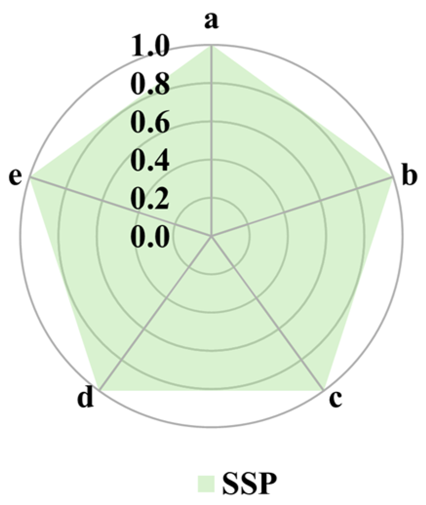
2.3.5. Construction of a Multi-Dimensional Landscape Connectivity Index

The radar chart serves as an effective tool for visualizing multi-dimensional data. In this study, we constructed radar charts to depict the FLC indices (Figure 3) and calculated the area enclosed by indices for each scenario to derive respective MLCI values. This analysis enabled us to determine the prioritization of development scenarios for FC.

Normalization: We applied the extreme value standardization method (Equation (2)) to normalize the FLC indices, limiting the range to [0.1, 1] [50]. Higher values of CA and CONNECT indices are beneficial for FC development, while higher values of PD, DIVISION, and ENN_MN indices are detrimental. To simplify the calculation of the radar chart area, we took the reciprocal of the PD, DIVISION, and ENN_MN indices to normalization (Equation (3)).

$$X=\mathrm{a}+(1-a)\times (X_i-X_{min})/(X_{max}-X_{min})$$

(2)

$$X=\mathrm{a}+(1-a)\times (1/X_i-1/X_{max})/(1/X_{min}-1/X_{max})$$

(3)

where X stands for the result of normalization. X_i represents the value to be normalized. X_min denotes the minimum value for normalization. X_max signifies the maximum value for normalization. a is a constant in the range from 0 to1, which is taken as 0.1 in this study.

Calculation of the radar chart area: We utilized the normalized FLC indices as dimensional values in radar graphs, and then employed Equation (4) to calculate the enclosed areas [17].

$$S=(ab+bc+cd+de+ea)\times \sin \alpha /2$$

(4)

where S refers to the enclosed area of five dimensions in the radar chart. a, b, c, d, and e separately stand for the values (FLC index values) of the dimension in the radargram. α (α = 360°/5) denotes the angle between two dimensions.

The disparate sort modes for the five indices lead to different results. Accordingly, we averaged the sum of all possible areas (the size of areas was determined by the summation of pairwise FLC index value multiplications) (Equation (5)) [17]. This value acts as a screening criterion for forest priority scenarios and is defined as the MLCI. A higher MLCI value signifies the superior performance of indices within a scenario, denoting increased suitability for future FC development.

$$MLCI=ab+bc+cd+de+ea+ac+ce+eb+bd+da$$

(5)

3. Results

3.1. Analysis of Land Use/Cover Change from 2000 to 2030

To validate the reliability of the PLUS model, we utilized the LUC data of 2000 and 2010 to simulate the 2020 data. Figure 4 shows that the simulated result is generally consistent with the observed LUC in 2020, with few differences. The Kappa coefficient is 0.932, the OA amounts to 96.2%, and the FoM coefficient is 0.164, which fulfills the requirement of accuracy. In conclusion, the PLUS model exhibits a favorable performance in LUC simulation, making it a reliable modeling tool.

Figure 5 illustrates the LUCC trends from 2000 to 2020. The results highlight that forest is the dominant LUC type in Fujian Province, accounting for over 62% in the past two decades. However, a discernible temporal decline in forests is observed, accompanied by a muted dynamic degree of single land use. Particularly, between 2000 to 2010, the K value is −0.06% (Figure 6), and 1134.160 km² of forest is primarily converted to built-up land (57.2%) and grassland (29.9%). From 2010 to 2020, the K value is −0.03%, and forest transferred 376.040 km² to built-up land (64.4%), cropland (15.6%), and grassland (13.4%). Employing the PLUS model, we project the LUC in 2030 under SSPs and discover that FC will increase in SSP1 and SSP4 (Figure 6). Specifically, by 2030, the global LUC structure remains essentially consistent under five SSPs, with FC accounting for over 61.4%. Notably, a decreasing trend in FC is observed for SSP2, SSP3, and SSP5. Consequently, SSP1 and SSP4 are more conducive to future FC developments in this aspect. In the periods of 2020 to 2030, SSP1 exhibits a K value of 0.04% and is projected to increase by 268.519 km² in the FC area. This growth stems from conversions of cropland (99.6%) and unused land (0.4%). For SSP4, with a K value of 0.2%, the FC area is expected to expand by 1793.725 km², primarily driven by conversions from cropland (63.6%) and grassland (36.0%).

3.2. Comparison of Forest Landscape Connectivity Indices at the Global Scale

The analysis of the index changes from 2000 to 2030 reveals optimization potential across all SSPs (Figure 7). The CA index displays growth trends exclusively for SSP1 and SSP4, with the latter showing a more significant increase. The PD index demonstrates upward trends in all five scenarios, notably peaking in SSP4 followed by SSP1. The DIVISION index decreases in both SSP1 and SSP4, with the most substantial decline observed in SSP1. The ENN_MN index exhibits notable decreases in all scenarios, with the more pronounced reductions seen in SSP1 and SSP4. At the threshold of 90 m, the CONNECT index remains stable in SSP4, but displays upward trends in other scenarios. However, at thresholds of 300, 600, and 1200 m, all scenarios exhibit decreasing trends. This analysis suggests that, in SSP1, the increase in PD and ENN_MN indices indicates that FC tends to be fragmented and the distance between patches elevated. In SSP2, the decline in the CA index alongside increases in PD and DIVISION indices signifies a reduced FC area and heightened fragmentation in the future. In SSP3, reductions in CA and CONNECT indices coupled with increases in PD and DIVISION indices point to FC area decrease, fragmentation intensification, and connectivity weakening. In SSP4, the increase in the PD index underscores an escalation of forest fragmentation. In SSP5, the decline in CA and most thresholds of CONNECT indices, coupled with the rise in PD and DIVISION indices, signifies a reduction in the FC area, an intensification of forest fragmentation, and a decrease in connectivity.

In this study, Equation (2) was employed to standardize the CA and CONNECT indices for 2030, while Equation (3) was utilized to normalize the PD, DIVISION, and ENN_MN indices to eliminate discrepancies in magnitude among various indicators. Subsequently, we combined the CONNECT index of four thresholds separately with the other FLC indices to construct radar charts (Figure 8), which revealed SSP4 as the scenario with the most frequent occurrence of the highest MLCI values (Figure 8e). In SSP1, the MLCI values consistently remain high across different thresholds, with a value of 2.569 at the 90 m threshold and 2.134 for the remaining three thresholds. Conversely, SSP2 and SSP3 exhibit similar yet lower MLCI values. At the 90 m threshold, the MLCI values are forecast to be 1.023 for SSP2 and 0.813 for SSP3. For SSP4, the MLCI values are particularly notable at the 300, 600, and 1200 m thresholds reaching 2.207, 2.183, and 2.302, respectively. Even at the 90 m threshold, its MLCI value of 2.092 ranks second, only surpassed by SSP1. In SSP5, the MLCI values at the 300, 600, and 1200 m thresholds are predicted to be 0.906, 0.879, and 0.913, respectively, representing the lowest values among these thresholds. At the global scale, through comprehensive comparisons of both single and multiple dimensions, SSP4 can be considered as the most prominent scenario for fostering FC development.

3.3. Comparison of Forest Landscape Connectivity Indices at the Local Scale

Employing the semi-variogram model, we identified the optimal moving window side length and subsequently calculated the FLC indices under SSPs from 2020 to 2030. The optimal development scenario at the local scale is identified as SSP4 (Figure 9). As depicted in Figure 10, SSP4 stands out prominently across all indices. Regarding the CA index, both the mean (28.202) and median (32.310) values for SSP4 surpass the other scenarios, indicating a larger FC area. While SSP1 demonstrates a suboptimal performance, there remains space for enhancement. Conversely, SSP2, SSP3, and SSP5 exhibit lower index distributions. Analysis of the PD index reveals that both SSP1 (2.929) and SSP4 (2.923) have higher mean values, signifying a greater degree of patch fragmentation in these scenarios. The remaining scenarios exhibit relatively lower levels of fragmentation. Analysis of the DIVISION index reveals that SSP4 shows the lowest median (0.482) and mean (0.500) values, indicating a low degree of separation. SSP1 performs suboptimally, whereas the remaining three scenarios exhibit a higher degree of separation. In terms of the ENN_MN index, SSP4 showcases the smallest maximum (120.000), median (79.155), and mean (107.547) values, reflecting optimized distances between patches. Similarly, SSP1 displays lower values, while the other scenarios display resemblances and higher distributions. In terms of the CONNECT index, each scenario’s performance varies across different thresholds. At the thresholds of 90 and 300 m, the mean values of SSP1 are 24.695 and 43.967, respectively, demonstrating a relatively high level of connectivity. Meanwhile, the mean values of SSP4 are 24.054 and 42.174, closely following SSP1. However, at the 600 m threshold, the mean values are all within the range of 50 to 55, and at the 1200 m threshold, the mean values are all between 60 and 66, implying minimal disparities in connectivity among scenarios. Overall, SSP4 exhibits optimization trends across multiple indices that positively influence local FC development. Nevertheless, the poor performance of the PD index underscores the need for ongoing attention to the issue of patch fragmentation in this scenario. Although SSP1 excels in specific indices, its overall optimization efficiency is relatively low. SSP2 faces challenges with high separation and increased distances between patches. SSP3, except the PD index, shows a poor performance across other indices, highlighting a critical need to improve the optimization efficiency of its FLC indices. Finally, in SSP5, the lower CA and higher DIVISION indices indicate a decrease in the local FC area and an increase in separation.

The mean and median values of FLC indices were normalized using Equations (2) and (3). Subsequently, a series of radar plots was constructed based on the threshold settings for the CONNECT indices, from which the MLCI values were calculated to assess the forest development prospects under each scenario (Figure 11a–d). The results reveal that, at the local scale, SSP4 exhibits significant superiority. Specifically, the radar chart constructed using mean values indicates that the MLCI values of SSP1 consistently remain high at 3.111 across all thresholds. In contrast, SSP2 demonstrates the lowest averaging MLCI value of 0.579 across all scenarios. While the MLCI values of SSP3 show minimal variation, they are generally low, averaging around 0.629. Compared with the other scenarios, SSP4’s MLCI values are significantly higher across all thresholds, specifically at 6.219, 4.189, 3.907, and 4.413. SSP5 also displays low MLCI values, but slightly higher values than SSP3 at all thresholds. Analysis of the radar chart based on median values reveals that SSP1 also maintains relatively high MLCI values across all thresholds. Specifically, the MLCI value at the 90 m threshold is 3.457 and the subsequent thresholds are all at 5.762. Notably, SSP4 stands out with its exceptional performance, boasting MLCI values of 7.573 at the 600 and 1200 m thresholds. Conversely, SSP2, SSP3, and SSP5 exhibit low MLCI values across all thresholds. A comprehensive analysis of both mean and median values underscores SSP4’s significant advantage in FLC development prospects. This result aligns with the findings from single-indicator analysis and further supports the argument that SSP4 is conducive to FC development at the local scale. Therefore, prioritizing SSP4 as the future development scenario can promote the sustained growth and optimization of FC.

4. Discussion

FC, as an essential component of natural ecosystems, not only provides a multi-fundamental service, but also plays a key role in climate regulation. The different configurations of LUC planning and FLC can profoundly impact on the distribution of FC, thereby influencing the quality of the ecological environment [1,51]. Hence, identifying the optimal development scenario for FC is essential to foster its sustainable and robust growth. Inspired by Liu et al. [17], who introduced a high-precision method for identifying multi-dimensional poverty in rural areas, this study developed the MLCI and identified SSP4 as the most suitable for the future development of FC in Fujian Province. Regarding methodological rationality, we employed the Kappa coefficient, OA, and FoM coefficient to test the reliability of the PLUS model under SSPs. Both the Kappa coefficient (0.932) and OA (96.2%) are considerable. Despite the FoM value not being high, it is noteworthy that Chen et al. reported an FoM coefficient range from 12% to 18% for the dynamic modeling of urban land use, while Pontius et al. also indicated that most FoM values are less than 30% [52,53]. Therefore, the FoM value of 0.164 obtained in this study is deemed acceptable. Additionally, we created radar charts using the mean and median values of FLC indices, with the consistency between these two outcomes. In terms of scenario construction, SSP4 is characterized by developmental differentiation, with middle-income and high-income regions showing a stronger focus on the ecological environment. Given Fujian Province’s substantial GDP, this scenario holds promising prospects for the advancement of its FC. In the aspect of FC, SSP1 and SSP4 demonstrate growing trends, whereas in the other scenarios, they exhibit declines. This result aligns with the research of Tang et al. [25], which also observed a substantial conversion of land to forests and other ecological uses under SSP1 and SSP4. From this perspective, both SSP1 and SSP4 exhibit high suitability. Specifically, FC increases significantly in SSP4 between 2020 and 2030, expanding by 1793.725 km², while in SSP1, the increase is relatively moderate at 268.519 km². There is essentially no diversion of forests to other land use in SSP1, while some forests are converted to cropland in SSP4 (+329.479 km²). In both scenarios, the primary source of forest is converted from cropland, with the transfer amount in SSP4 exceeding SSP1 by 1084.636 km². Consequently, SSP4 proves more advantageous than SSP1 in terms of FC development. Further analysis of the FLC indices reveals that multiple indices under SSP4 exhibit superiority. This indicates that, in this scenario, not only does FC increase in Fujian Province, but its FLC is also optimized, which is significant for maintaining the integrity and functionality of ecosystems.

Despite possessing certain advantages of FC development under SSP4, it still exhibits deficiencies in LUC structure and FLC indices. Specifically, by 2030, while SSP4 is projected to expand forest areas by 2126.533 km², 332.807 km² of forest that converts into cropland (99.0%) and built-up land (1.0%) exist. This conversion phenomenon primarily occurs in the southern Fujian Province, with a higher likelihood in Putian, Quanzhou, and Xiamen (Figure 6). Moreover, in SSP4, although most connectivity indices show an excellent performance by 2030, it is noteworthy that the PD index experiences a significant increase compared to 2020. This rise reflects an intensification of FC fragmentation, which is pronounced not only at the global scale, but also locally, with poor performances compared to other scenarios (Figure 7 and Figure 11). Such a trend of fragmentation may have adverse effects on the development of FC, thereby impeding the realization of its full ecological service potential.

Upon a comprehensive assessment of various indicators, it has been concluded that SSP4 is the preferred option for FC development in Fujian Province. However, in formulating forest development policies based on SSP4, it is imperative to focus on reducing the conversion rate of forests and optimizing the PD index. To achieve this goal, the following strategies are proposed: (1) Enhance forest quality and ecological functions through improved forest cultivation and increased tree species diversity; (2) Strengthen ecological restoration to boost the forest’s water retention and soil conservation capabilities, ensuring the stability and vitality of the forest ecosystem; (3) Heighten forest protection and management to combat illegal logging and destruction, ensuring the sustainable utilization of forest resources; and (4) Enhance forest connectivity and reduce fragmentation by optimizing forest road construction and augmenting vegetation cover. Based on the LUC projections in SSP4, a partial conversion of forest to cropland is to occur from 2020 to 2030. Therefore, an active policy of converting cropland back to forest is essential to facilitate the continued advancement of FC development. Additionally, the PD index displays an upward trend in Fuzhou and Ningde (Figure 12). Consequently, it is crucial to closely monitor the changes in PD in these two areas and make efforts to minimize fragmentation when implementing the FC development strategy in Fujian Province under SSP4. Although this study’s MLCI analysis model focuses on Fujian Province, its analytical framework and methodology offer novel insights into FC development in diverse regions. Therefore, this model can serve as a valuable guide and reference for FC development in other regions.

Due to data acquisition limitations, this study selected 10 available and qualifiable driving factors. Additionally, FCC is also influenced by complex interplays of numerous elements, including soil physicochemical properties and solar radiation. Given the intricacy of the driving factors for FCC, it is currently challenging to incorporate all influencing elements. Hence, in the subsequent research, it is necessary to analyze more driving factors to comprehensively reveal the intrinsic mechanisms of FCC. When employing the PLUS model for predictions, influenced by LEAS, the expansion of FC is impacted by historical trajectories. However, the overall space is limited, meaning that forests cannot perpetually encroach on other land types. Therefore, as formulating model assumptions, it is crucial to incorporate specific conditions, such as setting agricultural and ecological land red line and urban development boundaries. Moreover, we only selected five SSPs in this study. In combination with representative concentration pathways (RCPs) [19], we should design distinct scenarios for respective subareas to make the simulations more realistic and specific in future studies.

5. Conclusions

This study employed the SSPs framework and the PLUS model to predict FCC in 2030. Additionally, we calculated the FLC indices at both global and local scales, and constructed the MLCI to identify the most favorable FC development scenario. The conclusions are as follows:

(1)

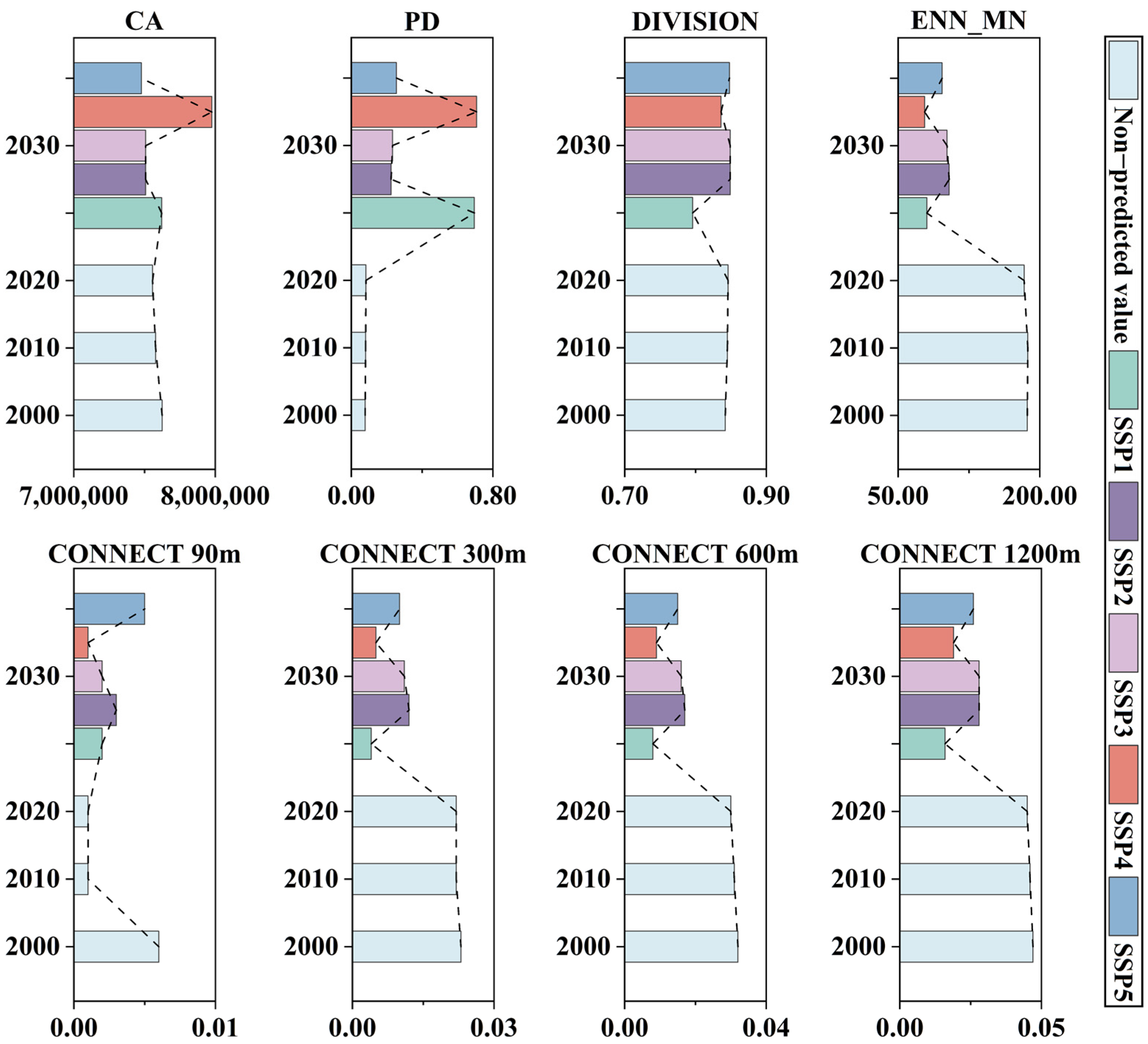
By 2030, the FC in all scenarios is projected to surpass 61.4%, with growth observed only in SSP1 (+268.519 km²) and SSP4 (+1793.725 km²), while reductions were evident in SSP2 (−220.938 km²), SSP3 (−219.558 km²), and SSP5 (−520.379 km²). Notably, forest in SSP1 is primarily converted from cropland (99.6%), with the transformation predominantly occurring in Longyan and the northwest of Zhangzhou, Putian, and Quanzhou. In SSP4, the main forest transfers involve cropland (63.6%) and grassland (36.0%). Additionally, the forest loss in SSP4 amounts to 332.807 km², with over 99.9% converted to cropland.

(2)

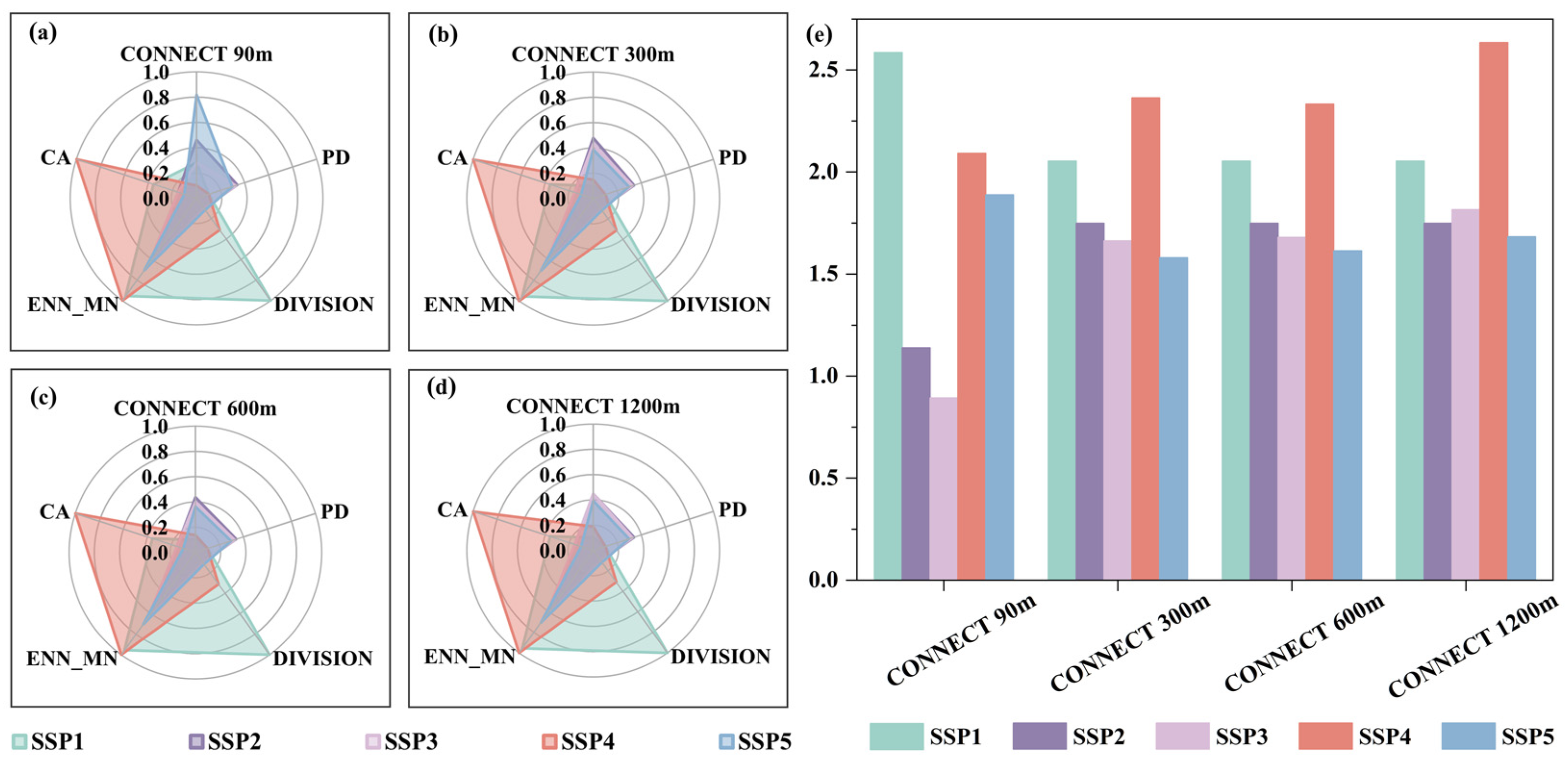
At a global scale, SSP4 outperforms the other scenarios. From 2020 to 2030, SSP4 consistently achieves high MLCI values across all thresholds. Specifically, at the CONNECT 90 m threshold, SSP1 attains the highest MLCI value of 2.569, followed by SSP4 at 2.092. At the 300, 600, and 1200 m thresholds, SSP4 records the highest MLCI values of 2.207, 2.183, and 2.302, respectively.

(3)

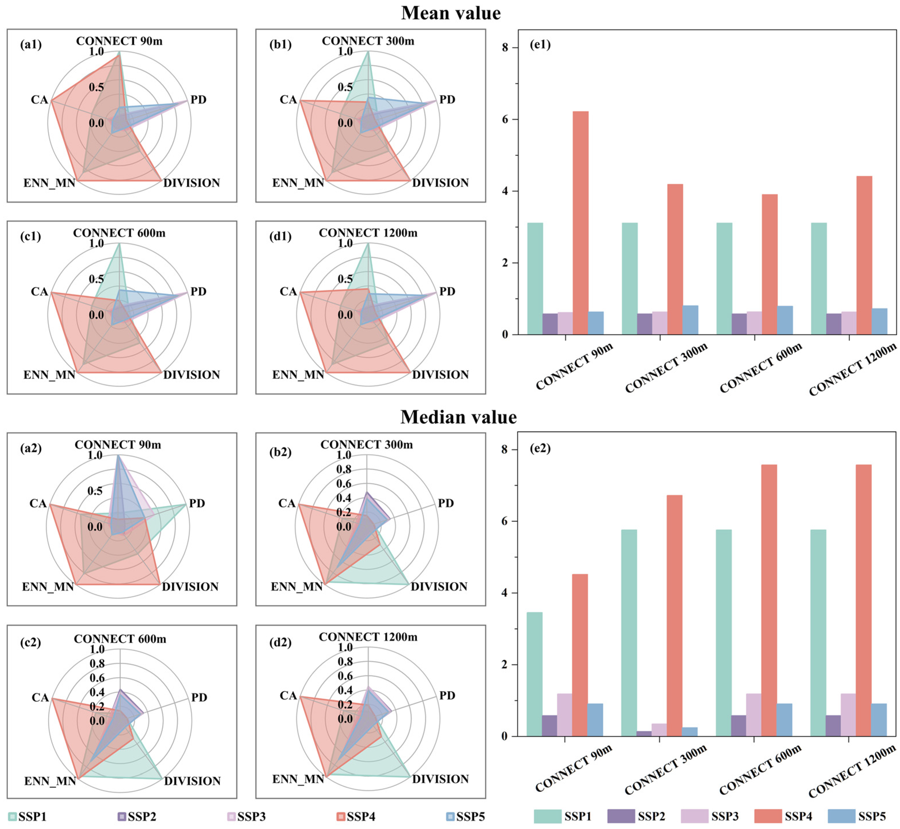
At a local scale, SSP4 also demonstrates significant superiority. When assessing MLCI values based on the mean FLC indices, SSP4 (3.907–6.219) consistently achieves the highest values across all thresholds, followed by SSP1 (3.111), and the lowest is SSP2 (0.579). Similarly, when considering MLCI values derived from the median FLC indices, SSP4 (4.519–7.573) maintains the highest value, surpassing SSP1 (3.457–5.762) that follows it, and the lowest value of SSP3 (0.354–1.188).

The superior performance of SSP4 at both global and local scales suggests a comprehensive enhancement in FLC indices, which is beneficial for the future development of FC. In conclusion, these findings hold significant implications for guiding future FC layouts and advancing the sustainable development of forest ecosystems.

References

1. Liu, S.; Dai, M.; Wen, Y.; Wang, H. A review on forest ecosystem management towards ecosystem services: Status, challenges, and future perspectives. Acta Ecol. Sin. 2015, 35, 0001–0009. [Google Scholar]
2. Houballah, M.; Cordonnier, T.; Mathias, J.D. Which infrastructures for which forest function? Analyzing multifunctionality through the social-ecological system framework. Ecol. Soc. 2020, 25, 22. [Google Scholar] [CrossRef]
3. Li, Y.; Xiao, X.; Li, X.; Qin, Y.; Dong, J. Multi-scale assessments of forest fragmentation in China. Biodivers. Sci. 2017, 25, 372–381. (In Chinese) [Google Scholar] [CrossRef]
4. Department of Forest Resources Management. The seventh national forest resources inventory and forest resources status. For. Resour. Manag. 2010, 1, 1–8. (In Chinese) [Google Scholar] [CrossRef]
5. Cui, H.; Liu, M. Analysis on the results of the 9th national forest inventory. J. West China For. Sci. 2020, 49, 90–95. (In Chinese) [Google Scholar] [CrossRef]
6. Zou, L.; Wang, J.; Bai, M. Assessing spatial–temporal heterogeneity of China’s landscape fragmentation in 1980–2020. Ecol. Indic. 2022, 136, 11. [Google Scholar] [CrossRef]
7. Morán-Ordóñez, A.; Hermoso, V.; Martínez-Salinas, A. Multi-objective forest restoration planning in Costa Rica: Balancing landscape connectivity and ecosystem service provisioning with sustainable development. J. Environ. Manag. 2022, 310, 114717. [Google Scholar] [CrossRef]
8. Wang, X.; Zhao, C.; Yang, R.; Jia, H. Dynamic characteristics of sandy vegetation landscape pattern based on dimidiate pixel model. Trans. Chin. Soc. Agric. Eng. 2016, 32, 285–294. [Google Scholar] [CrossRef]
9. Deng, Z.; Quan, B.; Zhang, H.; Xie, H.; Zhou, Z. Scenario simulation of land use and cover under safeguarding ecological security: A case study of Chang-Zhu-Tan Metropolitan Area, China. Forests 2023, 14, 2131. [Google Scholar] [CrossRef]
10. Cai, G.; Lin, Y.; Zhang, F.; Zhang, S.; Wen, L.; Li, B. Response of ecosystem service value to landscape pattern changes under low-carbon scenario: A case study of Fujian Coastal Areas. Land 2022, 11, 2333. [Google Scholar] [CrossRef]
11. Hayes, J.J.; Robeson, S.M. Spatial variability of landscape pattern change following a ponderosa pine wildfire in northeastern New Mexico, USA. Phys. Geogr. 2009, 30, 410–429. [Google Scholar] [CrossRef]
12. Zhang, W.; Yuan, Q.; Cai, H. Unravelling urban governance challenges: Objective assessment and expert insights on livability in Longgang District, Shenzhen. Ecol. Indic. 2023, 155, 110989. [Google Scholar] [CrossRef]
13. Chen, J.; Chen, S.; Fu, R.; Wang, C.; Li, D.; Jiang, H.; Zhao, J.; Wang, L.; Peng, Y.; Mei, Y. Simulation of water hyacinth growth area based on multi-source geographic information data: An integrated method of WOE and AHP. Ecol. Indic. 2021, 125, 107574. [Google Scholar] [CrossRef]
14. Yuan, Y.; Wang, M.; Zhu, Y.; Huang, X.; Xiong, X. Urbanization’s effects on the urban-rural income gap in China: A meta-regression analysis. Land Use Policy 2020, 99, 104995. [Google Scholar] [CrossRef]
15. Cunha-Zeri, G.; Guidolini, J.F.; Branco, E.A.; Ometto, J.P. How sustainable is the nitrogen management in Brazil? A sustainability assessment using the Entropy Weight Method. J. Environ. Manag. 2022, 316, 115330. [Google Scholar] [CrossRef]
16. Hu, X.; Xu, C.; Chen, J.; Lin, Y.; Lin, S.; Wu, Z.; Qiu, R. A synthetic landscape metric to evaluate urban vegetation quality: A case of Fuzhou City in China. Forests 2022, 13, 1002. [Google Scholar] [CrossRef]
17. Liu, Y.; Xu, Y. Geographical identification and classification of multi-dimensional poverty in rural China. Acta Geogr. Sin. 2015, 70, 993–1007. [Google Scholar] [CrossRef]
18. Su, F.; Xu, Z.; Shang, H. An Overview of Sustainable Livelihoods Approach. Adv. Earth Sci. 2009, 24, 61–69. [Google Scholar] [CrossRef]
19. IPCC. Climate Change 2014: Impacts, Adaptation, and Vulnerability; Cambridge University Press: Cambridge, UK; New York, NY, USA, 2014. [Google Scholar]
20. O’Neill, B.C.; Kriegler, E.; Ebi, K.L.; Kemp-Benedict, E.; Riahi, K.; Rothman, D.S.; van Ruijven, B.J.; van Vuuren, D.P.; Birkmann, J.; Kok, K.; et al. The roads ahead: Narratives for shared socioeconomic pathways describing world futures in the 21st century. Glob. Environ. Chang. 2017, 42, 169–180. [Google Scholar] [CrossRef]
21. Chen, J.; Liu, Y.; Pan, T.; Liu, Y.; Sun, F.; Ge, Q. Population exposure to droughts in China under the 1.5 °C global warming target. Earth Syst. Dyn. 2018, 9, 1097–1106. [Google Scholar] [CrossRef]
22. Li, M.; Zhou, B.; Gao, M.; Chen, Y.; Hao, M.; Hu, G.; Li, X. Spatiotemporal dynamics of global population and heat exposure (2020–2100): Based on improved SSP-consistent population projections. Environ. Res. Lett. 2022, 17, 094007. [Google Scholar] [CrossRef]
23. Jing, C.; Su, B.; Chao, Q.; Zai, J.; Wang, Y.; Tao, H.; Jiang, T. Projection of urbanization and economy in the ‘Belt and Road’ countries based on the shared socioeconomic pathways. China Popul. Resour. Environ. 2019, 29, 21–31. [Google Scholar]
24. Jiang, T.; Su, B.; Wang, Y.; Wang, G.; Luo, Y.; Zai, J.; Huang, J.; Gao, M.; Lin, Q.; Liu, S.; et al. Gridded datasets for population and economy under Shared Socioeconomic Pathways for 2020–2100. Clim. Chang. Res. 2022, 18, 381–383. [Google Scholar] [CrossRef]
25. Tang, Q.; Yu, P.; Chen, Z.; Bai, S.; Chen, Y. Simulation of land use change based on shared socioeconomic pathways. Res. Soil Water Conserv. 2022, 29, 301–310. [Google Scholar] [CrossRef]
26. Van Dessela, W.; Van Rompaeya, A.; Szilassib, P. Sensitivity analysis of logistic regression parameterization for land use and land cover probability estimation. Int. J. Geogr. Inf. Sci. 2011, 25, 489–508. [Google Scholar] [CrossRef]
27. Wu, H.; Li, Z.; Clarke, K.C.; Shi, W.; Fang, L.; Lin, A.; Zhou, J. Examining the sensitivity of spatial scale in cellular automata Markov chain simulation of land use change. Int. J. Geogr. Inf. Sci. 2019, 33, 1040–1061. [Google Scholar] [CrossRef]
28. Basse, R.M.; Omrani, H.; Charif, O.; Gerber, P.; Bódis, K. Land use changes modelling using advanced methods: Cellular automata and artificial neural networks. The spatial and explicit representation of land cover dynamics at the cross-border region scale. Appl. Geogr. 2014, 53, 160–171. [Google Scholar] [CrossRef]
29. Li, X.; Chen, G.; Liu, X.; Liang, X.; Wang, S.; Chen, Y.; Pei, F.; Xu, X. A new global land-use and land-cover change product at a 1-km resolution for 2010 to 2100 based on human-environment interactions. Ann. Am. Assoc. Geogr. 2017, 107, 1040–1059. [Google Scholar] [CrossRef]
30. Liang, X.; Guan, Q.; Keith, C.; Liu, S.; Wang, B.; Yao, Y. Understanding the drivers of sustainable land expansion using a patchgenerating land use simulation (PLUS) model: A case study in Wuhan, China. Comput. Environ. Urban Syst. 2021, 85, 101569. [Google Scholar] [CrossRef]
31. Li, Y.; Xia, Z.; Zhang, L. Carbon emission prediction and spatial optimization of land use in Chengdu-Chongqing economic circle in 2030 based on SSPs multi-scenarios. Ecol. Environ. Sci. 2023, 32, 535–544. [Google Scholar] [CrossRef]
32. Chen, Z.; Yu, P.; Chen, Y.; Jiang, S.; Bai, S.; Gu, S. Spatio-temporal changes of water resources ecosystem services in the Hanjiang River Basin based on the shared socioeconomic pathway. Chin. J. Eco-Agric. 2021, 29, 1800–1814. [Google Scholar] [CrossRef]
33. Fujian Provincial Bureau of Statistics. Statistical Bulletin on National Economic and Social Development of Fujian Province; Fujian Provincial Bureau of Statistics: Fuzhou, China, 2021.
34. Wang, B.; Liao, J.; Zhu, W.; Qiu, Q.; Wang, L.; Tang, L. The weight of neighborhood setting of the FLUS model based on a historical scenario: A case study of land use simulation of urban agglomeration of the Golden Triangle of Southern Fujian in 20. Acta Ecol. Sin. 2019, 39, 4284–4298. [Google Scholar]
35. Kebaili Bargaoui, Z.; Chebbi, A. Comparison of two kriging interpolation methods applied to spatiotemporal rainfall. J. Hydrol. 2009, 365, 56–73. [Google Scholar] [CrossRef]
36. Gao, J. Downscaling global spatial population projections from 1/8-degree to 1-km grid cells. In Enviromental Science, Geography; National Center for Atmospheric Research: Boulder, CO, USA, 2017. [Google Scholar] [CrossRef]
37. Zhen, Y.; Wu, Z.; Yin, Z.; Yang, X.; Zhao, X. Study on spatio-temporal change of land use in Zoige County, Sichuan Province. Ecol. Sci. 2022, 41, 41–49. [Google Scholar] [CrossRef]
38. Fu, J.; Cao, G.; Guo, W. Land use change and its driving force on the southern slope of Qilian Mountains from 1980 to 2018. Chin. J. Appl. Ecol. 2020, 31, 2699–2709. [Google Scholar] [CrossRef]
39. Cui, X.; Guo, Y. Analysis on the spatio-temporal dynamic evolution of land use structure of western urban agglomerations in the past 40 years. J. Arid Land Resour. Environ. 2022, 36, 16–24. [Google Scholar] [CrossRef]
40. Yao, Y.; Liu, X.; Li, X.; Liu, P.; Hong, Y.; Zhang, Y.; Mai, K. Simulating urban land-use changes at a large scale by integrating dynamic land parcel subdivision and vector-based cellular automata. Taylor Fr. 2017, 31, 2452–2479. [Google Scholar] [CrossRef]
41. Congalton, R.G. A review of assessing the accuracy of classifications of remotely sensed data. Remote Sens. Environ. 1991, 37, 35–46. [Google Scholar] [CrossRef]
42. Lin, J.; Li, X.; Li, S.; Wen, Y. What is the influence of landscape metric selection on the calibration of land-use/cover simulation models? Environ. Model. Softw. 2020, 129, 104719. [Google Scholar] [CrossRef]
43. Liang, X.; Liu, X.; Li, D.; Zhao, H.; Chen, G. Urban growth simulation by incorporating planning policies into a CA-based future land-use simulation model. Int. J. Geogr. Inf. Sci. 2018, 32, 2294–2316. [Google Scholar] [CrossRef]
44. Sun, J.; Zhang, Y.; Qin, W.; Chai, G. Estimation and Simulation of Forest Carbon Stock in Northeast China Forestry Based on Future Climate Change and LUCC. Remote Sens. 2022, 14, 3653. [Google Scholar] [CrossRef]
45. Li, X.; Bu, R.; Chang, Y.; Hu, Y.; Wen, Q.; Wang, X.; Xu, C.; Li, Y.; He, H. The response of landscape metrics against pattern scenarios. Acta Ecol. Sin. 2004, 24, 123–134. [Google Scholar]
46. Wu, J.; Shen, W.; Sun, W.; Tueller, P. Empirical patterns of the effects of changing scale on landscape metrics. Landsc. Ecol. 2002, 17, 761–782. [Google Scholar] [CrossRef]
47. Wu, J. Landscape ecology: Concepts and theories. Chin. J. Ecol. 2000, 19, 42–52. [Google Scholar] [CrossRef]
48. Hou, L.; Liu, T. Study on the landscape pattern of southwest transition zone from mountainous to hilly areas under the influence of multi-dimensional terrain factors: A case study of the middle and upper reaches of Fujiang River Basin. J. Ecol. Rural. Environ. 2020, 36, 741–751. [Google Scholar] [CrossRef]
49. Zhang, L.; Deng, C.; Kang, R.; Yin, H.; Xu, T. Josef Kaufmann, H. Assessing the responses of ecosystem patterns, structures and functions to drought under climate change in the Yellow River Basin, China. Sci. Total Environ. 2024, 929, 172603. [Google Scholar] [CrossRef]
50. Yang, H.; Zhao, X.; Wang, L. Review of data normalization methods. Comput. Eng. Appl. 2023, 59, 13–22. [Google Scholar] [CrossRef]
51. Lu, M.; Zhang, Y.; Liang, F.; Wu, Y. Spatial relationship between land use patterns and ecosystem services value—Case study of Nanjing. Land 2022, 11, 1168. [Google Scholar] [CrossRef]
52. Chen, Y.; Li, X.; Liu, X.; Ai, B. Modeling urban land-use dynamics in a fast developing city using the modified logistic cellular automaton with a patch-based simulation strategy. Int. J. Geogr. Inf. Sci. 2013, 28, 234–255. [Google Scholar] [CrossRef]
53. Pontius, R.G.; Boersma, W.; Castella, J.-C.; Clarke, K.; de Nijs, T.; Dietzel, C.; Duan, Z.; Fotsing, E.; Goldstein, N.; Kok, K.; et al. Comparing the input, output, and validation maps for several models of land change. Ann. Reg. Sci. 2008, 42, 11–37. [Google Scholar] [CrossRef]
Figure 1. The geographical location and the Köppen-Geiger climate classification of Fujian Province in southeast China. (a) Location and administrative divisions of the Fujian Province in China. (b) Koppen-Geiger climate classification of Fujian Province. (c) Elevation, latitude and longitude of Fujian Province. Note: Cwa: temperate, dry winter, hot summer; Cfa: temperate, no dry season, hot summer; Cfb: temperate, no dry season, warm summer.
Forests 15 01490 g001
Figure 2. Workflow of the study.
Forests 15 01490 g002
Figure 3. Composition and structure of the multi-dimensional landscape connectivity indices (MLCIs). Note: a, b, c, d, and e stand for the FLC index values.
Forests 15 01490 g003
Figure 4. Observed and simulated LUCs in 2020. (a) Observed LUC in 2020. (b) Simulated LUC in 2020. (c) Difference between observed and simulated LUCs in 2020. Note: A1 and A2: cases of observed LUC; B1 and B2: cases of simulated LUC; C1 and C2: cases of difference between observed and simulated LUCs; CL: cropland; F: forest; GL: grassland; WA: water area; BL: built-up land; UL: unused land.
Forests 15 01490 g004
Figure 5. Spatial distribution and transfer of LUCs from 2000 to 2020.
Forests 15 01490 g005
Figure 6. Predictions of spatial distribution and transfer of LUCs in multi-scenarios from 2020 to 2030, and dynamic degree of single land use (K) from 2000 to 2030. (ae) are spatial distribution and transfer of LUCs in SSP1–SSP5, respectively. (f) describes the dynamic degree of single land use. Note: S2020 and S2030 stand for LUCs in 2020 and 2030 in multi−scenarios, respectively. The values of 00–10, 10–20, and 00–20 represent the periods of 2000–2010, 2010–2020, and 2000–2020, respectively.
Forests 15 01490 g006
Figure 7. Changes in global FLC indices in multi-scenarios from 2000 to 2030. Note: CA: class area; PD: patch density; DIVISION: landscape division index; ENN_MN: mean nearest-neighbor index; CONNECT: connectance index. Non-predicted value: observed FLC indices for Fujian Province from 2000 to 2020.
Forests 15 01490 g007
Figure 8. Comparison of global MLCIs in multi-scenarios in 2030. Radar chart for the CONNECT 90 m threshold (a), 300 m threshold (b), 600 m threshold (c), and 1200 m threshold (d). The bar chart represents the area of the radar graph for each scenario—MLCI values (e).
Forests 15 01490 g008
Figure 9. Distribution of local FLC indices for SSP4 in 2030. Note: CA: class area; PD: patch density; DIVISION: landscape division index; ENN_MN: mean nearest-neighbor index; CONNECT: connectance index.
Forests 15 01490 g009
Figure 10. Changes in local FLC indices in multi-scenarios in 2030. Note: CA: class area; PD: patch density; DIVISION: landscape division index; ENN_MN: mean nearest-neighbor index; CONNECT: connectance index.
Forests 15 01490 g010
Figure 11. Comparison of local MLCIs in multi-scenarios in 2030. Radar charts for CONNECT 90 m threshold (a), 300 m threshold (b), 600 m threshold (c), and 1200 m threshold (d). Radar chart area in multi-scenarios (e). The bar chart represents the area of the radar graph under each scenario—MLCI values (e).
Forests 15 01490 g011
Figure 12. The distribution of PD index changes under SSP4 from 2020 to 2030. PD: patch density.
Forests 15 01490 g012