Article

Multi-Scenario Ecological Network Conservation Planning Based on Climate and Land Changes: A Multi-Species Study in the Southeast Qinghai–Tibet Plateau

1
Guangxi Key Laboratory of Forest Ecology and Conservation, Guangxi Colleges and Universities Key Laboratory for Cultivation and Utilization of Subtropical Forest Plantation, College of Forestry, Guangxi University, Nanning 530004, China
2
State Key Laboratory of Urban and Regional Ecology, Research Center for Eco-Environmental Sciences, Chinese Academy of Sciences, Beijing 100085, China
3
School of Mechanical Engineering, Guangxi University, Nanning 530004, China
*
Authors to whom correspondence should be addressed.
Forests 2024, 15(9), 1506; https://doi.org/10.3390/f15091506 (registering DOI)
Submission received: 15 July 2024 / Revised: 3 August 2024 / Accepted: 27 August 2024 / Published: 28 August 2024
(This article belongs to the Section Forest Ecology and Management)

Abstract

:
The Qinghai–Tibet Plateau ecosystem is fragile, experiencing rapid changes in land cover driven by both climate change and human activities, leading to habitat fragmentation and loss and resulting in biodiversity decline. Habitat ecological networks (HA-ENs) are considered effective solutions for habitat connectivity and biodiversity conservation in response to these dual drivers. However, HA-EN studies typically rely on current or historical landscape data, which hinders the formulation of future conservation strategies. This study proposes three future scenarios—improvement, deterioration, and baseline scenarios—focused on the southeastern Qinghai–Tibet Plateau (SE-QPT). The habitats of 10 species across three classes are extracted, integrating land use and climate change data into habitat ecological network modeling to assess the long-term dynamics of HA-ENs in the SE-QPT. Finally, conservation management strategies are proposed based on regional heterogeneity. The results show the following: Climate change and human activities are expected to reduce the suitable habitat area for species, intensifying resource competition among multiple species. By 2030, under all scenarios, the forest structure will become more fragmented, and grassland degradation will be primarily concentrated in the southeastern and western parts of the study area. Compared to 1985 (71,891.3 km2), the habitat area by 2030 is projected to decrease by 12.9% (62,629.3 km2). The overlap rate of species habitats increases from 25.4% in 1985 to 30.9% by 2030. Compared to the HA-EN control in 1985, all scenarios show a decrease in connectivity and complexity, with only the improvement scenario showing some signs of recovery towards the control network, albeit limited. Finally, based on regional heterogeneity, a conservation management strategy of “two points, two cores, two corridors, and two regions” is proposed. This strategy aims to provide a framework for future conservation efforts in response to climate change and human activities.

1. Introduction

Climate change and human activities have precipitated a crisis in biodiversity, leading to the loss and fragmentation of habitats for numerous species [1,2,3,4]. These global change factors are perceived as posing a significant threat to global biodiversity [5], negatively impacting nearly all taxonomic groups, encompassing birds [6] and mammals [7], amphibians [8,9], and plants [10]. The ecosystem of the Qinghai–Tibet Plateau (QTP) is under dual pressure from human activities and climate change. As one of the most unique and sensitive ecosystems on Earth, the QTP has experienced significant changes since the mid-20th century [11,12]. Taking proactive and comprehensive conservation measures to prevent habitat fragmentation and biodiversity loss has become an urgent and widespread concern in landscape planning and sustainable management.
Ecological networks are recognized as an effective tool for mitigating landscape fragmentation and promoting the preservation of threatened habitats and their inherent biological communities [13,14,15]. By optimizing the structure of ecological networks and identifying priority areas, regional biodiversity can be effectively maintained and stabilized. However, the effectiveness of these conservation efforts has been diminishing due to global changes. In response to this challenge, research related to ecological networks has evolved to encompass areas such as multi-layer ecological networks and future ecological network predictions. Scenario simulation serves as a crucial tool for predicting future development [16] and can furnish a theoretical foundation for natural resource planning and management [17,18]. The construction of multi-scenario ecological networks based on future multiple scenarios enables the formulation of protection plans and policies suitable for future climate change and land alterations, grounded in the monitoring of species habitat conditions and species dynamics.
The construction of ecological networks involves identifying ecological sources, constructing resistance surfaces, and extracting ecological corridors [19]. Ecological networks analysis typically involves the use of graph theory, where each node represents an ecological source and its spatial location, while ecological corridors connect two ecological sources [20,21]. These corridors generally indicate diffusion potential and possess attributes such as length and direction. In the context of biodiversity conservation, the identification of ecological sources is crucial and should be closely associated with the target species, thereby making species habitats the centerpiece of species conservation research [22]. However, the majority of prior studies have concentrated on a single species or a select few focal species [23,24]. Indeed, several studies have found that corridors identified for one species might not be effectively utilized by other species [25,26]. To improve biodiversity conservation more broadly, it is essential to establish a methodology that can address the functional connectivity needs of multiple species, which will play a critical role in advancing conservation research. Landscape connectivity refers to the extent to which the landscape facilitates or hinders movement between resource patches [27,28]. Enhancing landscape connectivity can foster animal migration, the spread of plant habitats, gene flow, and various other ecological functions of the landscape [29,30]. Therefore, connectivity is crucial for the survival of animal and plant populations and contributes to reducing the risk of extinction [31]. Furthermore, actions aimed at enhancing and preserving landscape connectivity are widely recognized as beneficial for adapting to climate change [1,32,33]. For instance, wildlife corridors serve a crucial role in bolstering the persistence and adaptability of species in the face of severe climate change [34].
Our goal is to establish a biodiversity conservation framework that effectively supports the protection of multi-species biodiversity in the face of global change, with a particular focus on the Plateau’s sensitivity to climate change and human activities. This framework utilizes past and future climate data, along with species distribution predictions, to identify suitable habitats for various species. Subsequently, based on land use prediction models, future land use changes are forecasted, and circuit theory is applied to establish habitat connectivity, thereby promoting the construction of long-term, multi-scenario, multi-species ecological networks. The framework enhances the integration of ecological network models with future data, and through multi-scenario ecological network analysis and comparison, develops biodiversity conservation strategies to address future global changes. The main contributions of this study include the following: (1) constructing a multi-scenario HA-EN that integrates climate and land change data of the study area, establishing spatial distribution patterns of habitats and ecological corridors for multiple species; (2) identifying expected ecological challenges under future scenarios through the analysis of research results, determining priority conservation areas in conjunction with current development trends, and ultimately formulating relevant ecological conservation strategies for reference.

2. Materials and Methods

2.1. Study Area

The study area, encompassing Lhasa, Nyingchi, and Shannan cities in the Tibet Autonomous Region, is situated in the southeastern Qinghai–Tibet Plateau (SE-QTP), covering approximately 223,600 km2 (Figure 1). At an average altitude of around 3500 m, the region experiences an annual average temperature ranging from 4 to 12 °C and an annual precipitation between 300 and 1200 mm. During the summer, the region experiences warmth and rainfall due to the influence of the southwest monsoon, carrying abundant moisture and heat from the Indian Ocean, contributing to a high level of biodiversity. With significant differences in elevation, the study area represents the most complete vertical natural zone for mountainous regions worldwide and serves as a crucial location for investigating global climate change. Nevertheless, against the backdrop of global warming, the temperature of the QTP has risen [35], leading to the accelerated retreat of glaciers, significant expansion of lakes, and increased glacial runoff, which have also caused major disasters such as avalanches and glacial lake outburst floods, and the potential risks of grassland degradation, ecological environment security, and water shortage may gradually increase in the future [36,37].

2.2. Data Sources

The data utilized in this study encompass geographical, socio-economic, and climatic data. All data are publicly available to ensure scalability of the experiments and models. To ensure data availability, all data in this study were converted to a uniform projected coordinate system with a uniform grid size of 200 × 200 m. Details are shown in Table 1.

2.3. Research Framework

The research framework of this paper is divided into three parts (Figure 2). Firstly, multi-scenario LULC in 2030 was conducted based on the future land use simulation model. Subsequently, we used the MaxEnt model to determine species habitats in both 1985 and 2030 as ecological sources. The resistance surface was constructed by integrating the minimum cumulative resistance model with multi-scenario LULC and temporal data. By leveraging circuit theory, we established the connectivity of species ecological sources to formulate multi-scenario ecological networks. Finally, we analyzed networks for the years 1985 and 2030 under various scenarios. A priority protection pattern was devised by considering both future scenarios and actual conditions.

2.4. Multi-Scenario Prediction of LULC

2.4.1. Future Land Use Simulation Model

Future land use simulation (FLUS) is a model for simulating land use change under human activity, natural influence, and future scenarios [18]. The model simulates land use change by defining a set of rules and conversion rules. Rules can be based on interactions between land use types, the influence of the surrounding environment, and decision-makers’ behavior. Currently, this method is widely used in urban expansion simulation [38,39] and land use simulation [40,41,42].
In this study, we selected an appropriate land use classification system based on the LULC classification and the study area’s size, and we classified LULC into six categories: cropland, forest, grassland, impervious surfaces, water body, and unused land. The driving factors were selected from the existing research on natural, economic, and social aspects [18,39]. We utilized the following 9 indicators in this study: DEM, slope, water distance, road distance, population density, night light data, NDVI, settlement distance, and soil type.
The land use map from the year 2000 served as the basis for generating the simulated map for 2015. The simulation results were compared with the actual land use map of 2015 to assess the accuracy of the simulation. We used the LULC data from the year 2000 to simulate the LULC data for 2015. By comparing the simulation results with the actual 2015 LULC data, we found that our model achieved a Kappa coefficient of 0.89. This indicates that the model can effectively simulate the real land use dynamics within the study area.

2.4.2. Multi-Scenario Setting

To assess the impact of different land use management models on the ecological environment and to provide scientific support for future land use planning and policy making, we simulated three scenarios: sustainable development, disregarding ecological protection, and maintaining the status quo. By analyzing the positive and negative effects of each scenario on the environment and ecosystem, we aim to explore the importance of protecting ecological land and guide practical land use decisions.
(1)
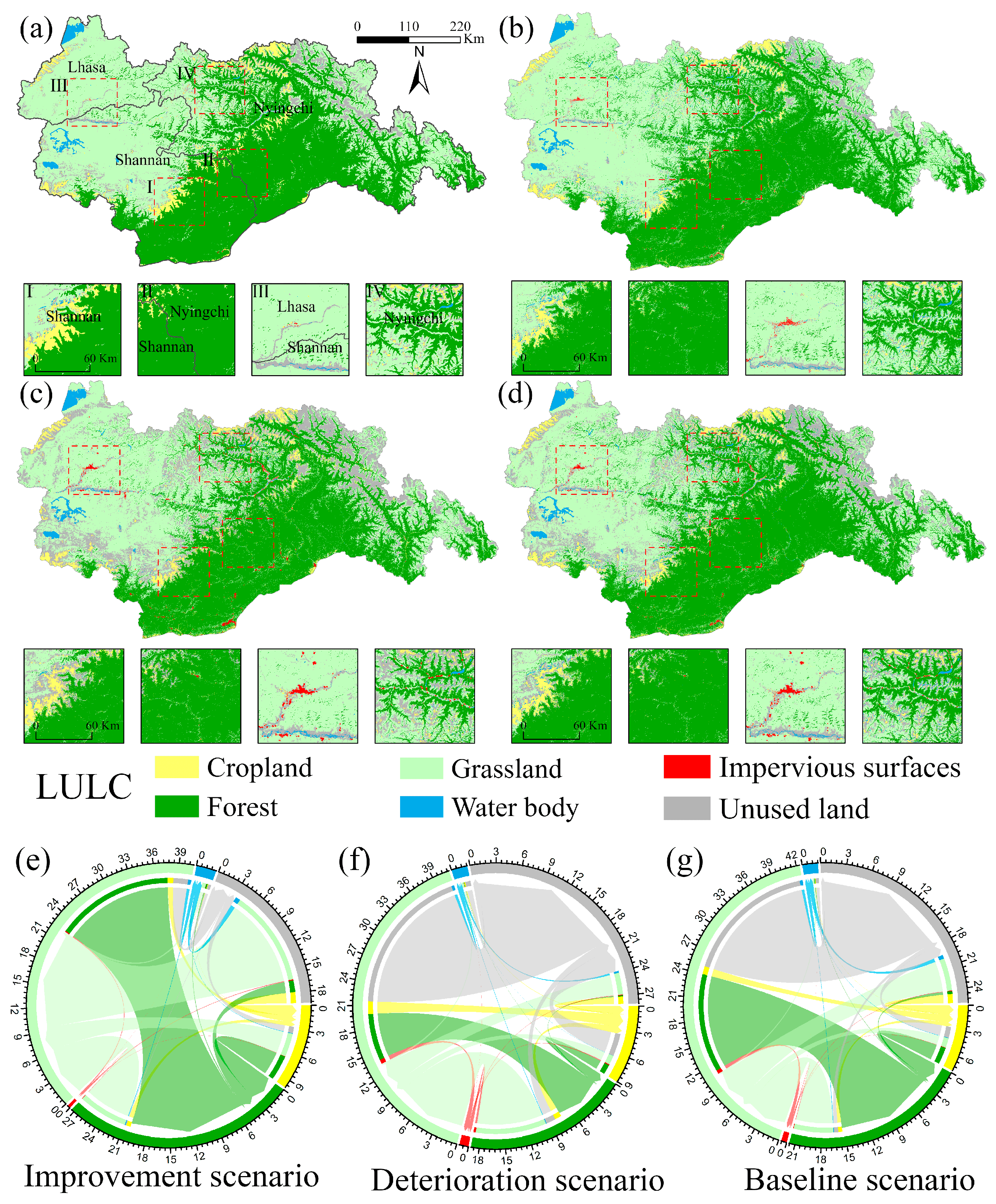
Improvement scenario: assume that forest land maintains its previous growth rate, grassland degradation is improved, and water bodies are designated as restricted conversion areas, while other land types convert randomly.
(2)
Deterioration scenario: abandon the protection of ecological land such as forests, grasslands, and water bodies, allowing these areas to be converted into other land types.
(3)
Baseline scenario: all land types continue their previous trends, with forest area increasing and grassland area continuing to decrease.

2.5. Construction of Multi-Scenario Ecological Networks

2.5.1. Identification of Ecological Source

In this study, we used the MaxEnt model to select habitats for species. The MaxEnt model is a machine learning model used to predict the potential distribution of species under different environmental conditions [43]. The MaxEnt model requires two types of data input: species distribution data and environmental variable data.
Based on previous research [44,45,46], we selected 19 bioclimatic data indicators as environmental variables. By excluding low-contribution and high-covariance environmental variables, 8 environmental variables were finally retained, and the specific environmental variable content is shown in Figure S1. The species distribution data came from the Global Biodiversity Information Facility (www.gbif.org) and field observation records. By combining the distribution and biological conservation status of species in Tibet, we selected 10 wild animals and plants from the IUCN Red List of Endangered Species and the National Key Protected Wild Animals and Plants List, including three birds (Grus nigricollis, Anser indicus, Nucifraga caryocatactes), three plants (Saussurea obvallata, Rhodiola crenulata, Rheum nobile), and four mammals (Catopuma temminckii, Martes flavigula, Capricornis sumatraensis, Budorcas taxicolor), with the spatial distribution as shown in Figure S2.
After fine-tuning the model parameters to obtain the probable distributions of the species, we reclassified the results of the species distribution probabilities into 5 categories using the natural breakpoint method and extracted the highest category as the ecological source.

2.5.2. Construction of Resistance Surface

Ecological resistance surface is the basis of ecological corridor extraction, which reflects the blocking effect of the landscape on material, energy, and species migration. Species behaviors such as migration, propagule dispersal, and gene exchange will be affected by natural conditions, human activities, etc., and will be concentrated in the characteristic diversity between different land use types and terrains. Therefore, we amalgamate previous methods of allocating habitat suitability predicated on land types [45,47] and couple multiple factors [48,49,50] to construct the resistance surface.
To simulate the ecological resistance pressures faced by species in different scenarios, we established ecological resistance surfaces for each of the four networks. Considering the impact of factors such as terrain, food, water sources, and human activities on wildlife and vegetation, we selected habitat quality, NDVI, road distance, elevation, and water source distance data to quantify the ecological resistance pressure faced by flora and fauna. Drawing from previous research, we categorized the resistance values for all factors into five levels (Table 2) and assigned values of 1, 5, 10, 20, and 50 based on increasing resistance values [45,51,52]. Finally, we used the minimum cumulative resistance model to integrate all resistance factors, creating an ecological resistance surface. The habitat quality calculation procedure is in Supplementary Materials.

2.5.3. Extraction of Ecological Corridor

We used the circuit theory model to establish the connectivity relationship between species habitats. The circuit theory model was initially applied to predict the genetic diversity of species and then gradually developed to predict the migration and diffusion processes of biological populations [53]. The circuit theory model establishes connections within complex landscapes and circuits, modeling the random walk characteristics of electrons in circuits, with ecological resistance surfaces represented as conductive surfaces. Circuit theory analogizes various components within complex landscapes (such as animals, plant reproductive bodies, etc.) to electrons. During movement, corridors with low resistance (low ecological barriers) imply a higher probability for species passage and are difficult to replace. Conversely, corridors with high resistance (high ecological barriers) indicate a lower probability of passage and insufficient stability [54].

2.6. Analysis of Multi-Scenario Ecological Networks

To further understand the impact of global change on the overall and local functions of ecological networks, we conducted network topology and species interaction analysis. In analyzing species interactions, this study began by examining the ecological sources, ecological corridor overlap, and intersection relationships among multiple species. The research involved calculating overlap areas, the number of intersections, and spatial relationships of species. In the network topology analysis, we abstracted the ecological sources as nodes and the ecological corridors as edges, and the structure of networks formed an undirected and unweighted complex network.
The network describes the spatial distribution and connectivity, and by observing and calculating the spatial characteristics of the entire ecological network, including edges and nodes, we can obtain the stability, stability, and importance of the source and node connections in the ecological network. In addition, discussing the topological characteristics of the ecological network from the perspective of complex networks helps to reveal the characteristics that traditional methods cannot determine and thus clarify the formation and evolution of the ecological network. In this study, five network topology indicators, namely, degree, average path length, clustering coefficient, betweenness centrality, closeness centrality, and eigenvector centrality, were used to describe multi-scenario ecological networks [48,49,50]. The concepts and calculation formulas of each indicator are shown in Table S2.

3. Results

3.1. Spatio-Temporal Changes of LULC Pattern in SE-QTP

Compared to the LULC situation in 1985, the forest structure in 2030 under each scenario is more fragmented. Grassland degradation is primarily concentrated in the southeast and west of the study area, and human activity impacts are most evident in the urban periphery and some southern areas of the study area. As shown in Figure 3, several significant features can be observed in the land use change from 1985 to 2030. Forest and grassland are the two main land use types in the study area, distributed in the south and west of the study area, respectively. In 1985, forests covered 42.6% of the study area, and the internal structure of the forest was largely intact with only a few fragmented areas. By 2030, under all scenarios, varying degrees of fragmentation appear in the forest. The forest proportions under the improvement and baseline scenarios were 46.0% and 45.6%, respectively, showing a slight increase. However, under the deterioration scenario, the forest area decreased to 41.1%, with much of the forest converting to grassland, cropland, and unused land.
In the deterioration scenario, the impervious surface proportion increased from 0.03% in 1985 to 0.43%. Due to the low population density of the study area, the spread of impervious surfaces mainly occurred from the central urban area. Notably, many forests in the southern part of the study area were converted into impervious surfaces, potentially harming the stability and connectivity of the forest interior.
Under the baseline scenario, the grassland proportion degraded to 38%, a 7% decrease compared to 1985, with grasslands mainly converting to unused land and forest. The most significant areas of grassland degradation were in the southeast and west of the study area, where the average elevation was above 4200 m, and the primary grassland type was alpine grassland. Therefore, the grassland degradation scenario predicted by this study aligns closely with the actual degradation situation.

3.2. Spatial Distribution of Ecological Network in SE-QTP

3.2.1. Spatial Distribution of Resistance Surface

From a spatial distribution perspective, the western and northern parts of the study area exhibit high resistance, while the central and southeastern parts show low resistance (Figure 4). The spatial distribution of resistance surfaces in 2030 under different scenarios is similar, with close resistance values. However, each scenario shows significant spatial differences compared to the resistance surfaces in 1985. In 1985, the highest resistance value was 37.7, while in 2030, under all scenarios, the highest resistance value for the improvement scenario was 41.5, lower than that of the degradation and baseline scenarios. The average resistance in the improvement scenario was 14.81, also lower than that of the degradation scenario (15.57) and baseline scenario (15.28).
From 1985 to 2030, resistance values in typical regions generally show an increasing trend, with the range of high-resistance areas expanding. Type I (mountainous and canyon crossing points) and Type II (forested areas) exhibit fragmentation of low-resistance areas, eventually evolving into large areas with moderate resistance values. Type III (urban areas) reflects changes in resistance surfaces due to rapid urban development, with urban areas becoming high-resistance zones. Type IV (grassland areas) shows continuous expansion of high-resistance areas, while low-resistance areas in grasslands continue to shrink. Compared to 1985, changes in resistance in typical regions under the improvement scenario in 2030 are less pronounced than those in the baseline and degradation scenarios. Changes in resistance surfaces indicate that habitats for flora and fauna will face increasing resistance values, leading to habitat loss and fragmentation, thereby threatening the stability of species populations and structure.

3.2.2. Spatial Distribution of Habitat Suitability

By 2030, both the total area and number of habitats will decrease (Table 3). Specifically, compared to 1985 (71,891.3 km2), the area of habitats in 2030 will decrease by 12.9% (62,629.3 km2). Among them, the distribution range of Rheum nobile will significantly decrease, approximately by 4259.0 km2. Next is Budorcas taxicolor, with a decrease of 3014.1 km2. At the same time, the overlap rate of species habitats will increase from 25.4% in 1985 to 30.9% in 2030, indicating that environmental changes will reduce the suitable habitat area for species and intensify the resource competition intensity among multiple species. However, environmental changes may be beneficial for the survival of individual species. For example, the distribution area of Rhodiola crenulata will increase by 2213.1 km2 by 2030; the habitat of Capricornis sumatraensis may increase by 688.8 km2 in the study area by 2030.

3.2.3. Spatial Distribution of Ecological Network

Figure 5 depicts the complete HA-EN under different scenarios (improvement, degradation, and baseline) for the study area in 1985 and 2030. The results reveal a dense spatial distribution pattern in the southeastern and northwestern parts of the study area, while connectivity is lacking in the western and northeastern parts. In 1985, the average corridor length was 62,589.3 m with an average resistance of 8.6, significantly lower than the values observed under all scenarios in 2030. Specifically, the average corridor length was 64,669.0 m for the improvement scenario, slightly less than 65,213.3 m for the baseline scenario and the maximum of 64,990.9 m for the degradation scenario. The ratio of habitat area to corridor crossing points reflects the intensity of species interactions. The results show the highest ratio in the baseline scenario (0.00808), followed by the degradation scenario (0.00782), with the lowest ratio observed in 1985 (0.00772). This indicates that environmental changes not only reduce suitable habitat area but also potentially increase the difficulty of species movement between habitats.
In typical regions (I-type: mountainous and canyon crossing points, II-type: forested areas, III-type: urban areas, and IV-type: grassland areas), significant reductions in habitat quantity and connectivity due to environmental changes are observed. Compared to 1985, the complexity of HA-EN substantially decreases under all simulated scenarios in 2030, highlighting the threat of habitat fragmentation to the stability of species populations and structure.

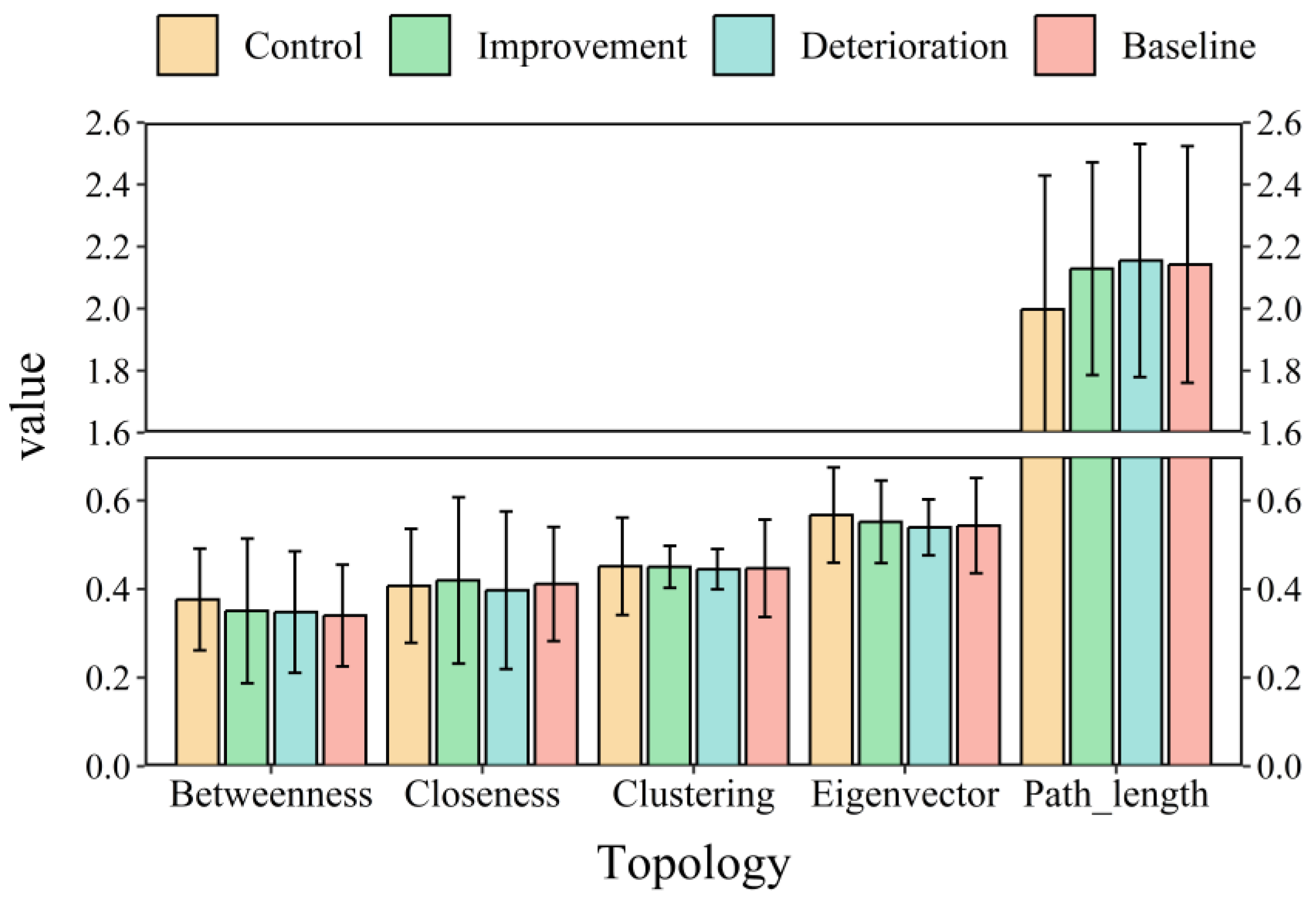
3.2.4. Changes in HA-EN Topology Indicators

Compared to 1985, the average path length in 2030 shows a significant increase in the deterioration and baseline scenarios, while it only slightly increases in the improvement scenario (Figure 6). Betweenness centrality in 1985 is significantly higher than in all scenarios for 2030. In 2030, the betweenness centrality of the improvement scenario is higher than that of the other two scenarios, with the baseline scenario being the lowest. Closeness centrality significantly decreases in the deterioration scenario, indicating that nodes in the network are increasingly deviating from the geometric center of the network, making the entire network more dispersed, while closeness centrality remains similar across the other three scenarios. The clustering coefficient is similar in 1985 and the improvement scenario, both higher than in the deterioration and baseline scenarios. Eigenvector centrality increases in 2030, suggesting a widening gap in node importance, with peripheral nodes becoming more dependent on central nodes due to the reduced importance of many nodes.
The clustering coefficient, reflecting the stability of the network nodes, was similar in the improvement network and the network in 1985, both higher than those of the deterioration and baseline networks. The eigenvector centrality, indicating the importance of the neighboring nodes of a node, increased in 2030, signifying a widening disparity in importance among nodes. Consequently, the periphery has become increasingly reliant on peripheral nodes, driven by the diminished significance of numerous nodes. Module analyses were performed for the network as a whole and for different species separately (Figure 7). In 1985, the network was divided into six modules, and in 2030, the number of modules was reduced to four for the deterioration and baseline networks and five for the improvement network. The reduction in modules reflects the fact that environmental changes in recent years have caused parts of the study area to become unsuitable for species, and species will move or congregate in new suitable habitats. Combined with topology results, from 1985 to 2030, the average degradation of network topology attributes was 4.1%. Compared to the baseline and deterioration networks, the topology of the improvement network increased by 1.6% and 2.2%.

4. Discussion

4.1. Discussion on Multi-Scenario Network

Given the profound influence of global change, the objectives and strategies for ecological restoration of national land vary under different development scenarios [18]. However, most existing research relies on current and historical landscape data, limiting the effectiveness of ecological network conservation in mitigating landscape fragmentation. Human activities and climate change, specifically LULC changes, determine the location and extent of habitat fragmentation and loss, as well as the likelihood of species traversing intermediate areas, thereby directly affecting the performance of ENs [55,56,57]. Static data may overlook future key changes and hotspot areas, failing to provide effective conservation strategies [58]. Assessing the potential impact of landscape changes on the structure and function of ENs is crucial for them to cope with landscape change disturbances. Zeller [59] noted that neglecting hotspot areas of change could result in misguided or ineffective conservation efforts. Bishop-Taylor [60] found that relying on static landscape priorities might lead to limited conservation budgets being misallocated to habitats that are not important for connectivity. Given limited resources and budgets, focusing on areas expected to change through multi-scenario simulations could be beneficial for long-term conservation. This dynamic and forward-looking analytical approach can more effectively guide the implementation of conservation measures, ensuring that ENs maintain their functionality and connectivity in the face of future climate change and land alteration [61]. Additionally, ongoing global climate changes will exacerbate the network cascading effects [62,63]. Predation, habitat, and reproduction relationships of species at regional scales are strongly interconnected, as are the impacts of global ecological cores, such as the Tibetan Plateau and the Amazon Rainforest, when subjected to climate change [62]. Consequently, scientists have begun to establish links between elements at the global scale through networks, which are used for tipping point analysis, early warning, detection, and prediction in dynamic systems [64].
The QTP, often referred to as the world’s “third pole” and “world water tower”, is primarily recognized for its unique advantages and the exceptional ecological value of its resources [12]. However, its distinctive geographical conditions render the QTP highly sensitive to global climate change, transforming it into a typically ecologically fragile area [65,66,67]. Over recent decades, global climate change has been rapidly and fiercely impacting the QTP, leading to an increasingly serious degradation of alpine grasslands and a gradual decrease in land productivity [11,12,68]. This poses a significant threat to the normal functioning of alpine grassland ecosystem services [69]. Furthermore, if the continued degradation of grasslands is allowed to persist, it will also pose a threat to the biodiversity of the alpine region [37]. Recognizing the immense harm caused by the ongoing degradation of grasslands should be a primary focus of ecological protection [70,71]. Therefore, our goal is to establish a framework to support efficient and effective planning of biodiversity under global change. This framework enhances the integration of ecological network models and future data and formulates biodiversity conservation plans that respond to future global change according to local conditions by analyzing long-term, multi-species, and multi-scenario ecological networks.

4.2. Multi-Scenario Conservation Pattern

In multi-scenario simulations, compared to the control network in 1985, the network indicators of three ecological networks in 2030 have changed to varying degrees. This clearly reflects the intensified ecological resource competition among animal and plant species due to human activities and environmental changes in recent years. The connectivity and stability of ecological networks have declined. The improvement and deterioration networks aim to align with the United Nations 2030 sustainable development plan and to find ecological problems from deterioration development. In our simulation results, the primary problem of the deterioration network is the significant increase in ecological resistance. Since we restricted the same correction factors, the increase in resistance is directly related to the change in LULC. Compared with the LULC in 1985, the forest and grassland proportions of the deterioration network both decreased, while the cropland, unused land, and impervious surface proportions increased. These proportion changes reflect the changes in land types caused by excessive logging and grazing, large-scale reclamation of farmland, and large-scale urban construction. Secondly, the deterioration network will aggravate the problem of landscape fragmentation. The deterioration network caused serious fragmentation of the forests in the south of Nyingchi and the south of Shannan due to large-scale urban construction, and then excessive logging and grazing and large-scale reclamation of farmland caused the ecological resistance of Lhasa and the north of Shannan to increase significantly, and the land structure became more fragmented. And large-area continuous habitats will be separated into small-area discontinuous habitat patches, forcing regional biodiversity to decline further.
The baseline scenario is grounded in the significant issue of grassland degradation that has persisted in the SE-QTP over recent decades. This scenario aligns with the observed trend in land changes within the study area in recent years. Among them, the most obvious change in land is the annual decline of grassland area, while the forest area keeps rising, so the baseline scenario more realistically reflects the current development trend of the study area. The most obvious area of grassland degradation in the baseline network is in Lhasa and the north of Shannan, where the average elevation is above 4200 m, classifying it as alpine grassland. Alpine grassland is very sensitive to environmental changes, and many studies have shown that alpine grassland is the most significant land type of grassland degradation in the QTP, and environmental conditions are the dominant factors affecting the stability of alpine grassland communities (Figure 8b). Therefore, protection measures should focus on studying the mechanism of grassland degradation caused by environmental conditions, while also controlling the impact of human activities on the growth environment. (Figure 8i) shows the direct harm of human development activities to grassland, and the deeper indirect harm caused by development should also be carefully considered, such as the impact of development on grassland water and heat conditions, soil conditions, and biological conditions. Secondly, some areas maintain a grazing lifestyle, and overgrazing leads to the decline of grassland biomass and soil nutrients, gradually causing grassland degradation (Figure 8j); in addition, rocky desertification directly destroys the grassland structure and causes irreversible damage (Figure 8g).
Compared to the other two scenarios, the implementation of the improvement network significantly improved the ecological conditions of the multi-species ecological network, moving closer to the network conditions of the 1985 control network. This includes a decrease in the length of ecological corridors, intersections, and ecological resistance values, an increase in network topology indicators, and a reduction in ecological resource competition pressure between species. In order to enhance the protection of biodiversity, we have integrated ecological issues and improvement measures from the three scenarios and have proposed protection interventions and policy suggestions. Ecological network and landscape connectivity play a key role in landscape planning and management policies and strategies [72,73]. The wild animals within the ecological network primarily inhabit the forests in the southern regions of Shannan and Nyingchi. The gradually expanding transportation network is detrimentally impacting the connectivity between animal habitats. During our field investigation, we observed the construction of protective barriers on both sides of the roads (Figure 8e). Although the protective net can reduce the occurrence of traffic accidents, the communication of terrestrial animals on both sides of the road will also be blocked. For this reason, governments and conservation organizations have built animal corridors to alleviate the serious damage and fragmentation of wildlife habitats caused by transportation facilities. This study identifies the intersections of roads and corridors and provides a reference for the spatial planning of wildlife corridors.
Summarizing all the above problems, we formulated the protection planning pattern of this study based on the baseline network: “two points, two cores, two belts, and two zones” (Table 4).

4.3. Shortcomings and Prospects

Given the complexity and long-term impacts of future scenarios, further research should consider more influencing factors and simulate different environmental change scenarios, such as farmland protection scenarios and ecosystem service enhancement scenarios. Additionally, since land policies vary across regions, land type simulations should align with the land policies of local decision-makers. In this study, because land use simulation is based on area changes, it is challenging to reflect more factors related to grassland quality degradation. However, the ultimate outcome of grassland quality degradation will evolve into desertification, characterized by changes in land type. Secondly, this study involves multiple species, selecting six plants and four animals (including two bird species) listed as endangered or protected globally and in China. These species exhibit a certain degree of similarity in their distribution points, leading to overlapping extracted ecological resources. We have only conducted a macro-level study of species habitat networks, and species-level analyses are still needed. Moreover, the ultimate goal of most spatial planning is to be applied in practical ecological protection; thus, more consideration should be given to issues that align with national policies, reality, effectiveness, and cost-efficiency. Finally, the SE-QTP is crucial for biodiversity conservation in East Asia and even Central Asia. Therefore, strengthening cooperation between China and its neighboring countries in establishing or managing transnational ecological protection and construction is wise. In future research, we will explore how to optimize the construction and management of HA-EN to better protect biodiversity. We hope these studies can provide more scientific evidence for biodiversity conservation and ecosystem management. With these improvements, future research will be able to more comprehensively assess the ecological environmental impacts under different scenarios, providing a solid foundation for formulating scientific and effective protection measures.

5. Conclusions

This study focuses on the SE-QTP, setting different scenarios to simulate the ecological space network of multi-species habitats and assess the impact of LULC and climate change on HA-EN. Based on the research results, we propose ecological protection schemes to address the challenges of spatio-temporal environmental changes. The main findings are as follows:
  • Resistance distribution characteristics: The western and northern parts of the study area exhibit high ecological resistance, while the central and southeastern parts exhibit low ecological resistance. With changes in climate and LULC, high-resistance areas continuously expand outward, and low-resistance areas continuously shrink. Under different scenarios, the ecological resistance of the improvement scenario is significantly better than that of the deterioration and baseline scenarios, yet there is still a significant difference compared to the baseline year of 1985.
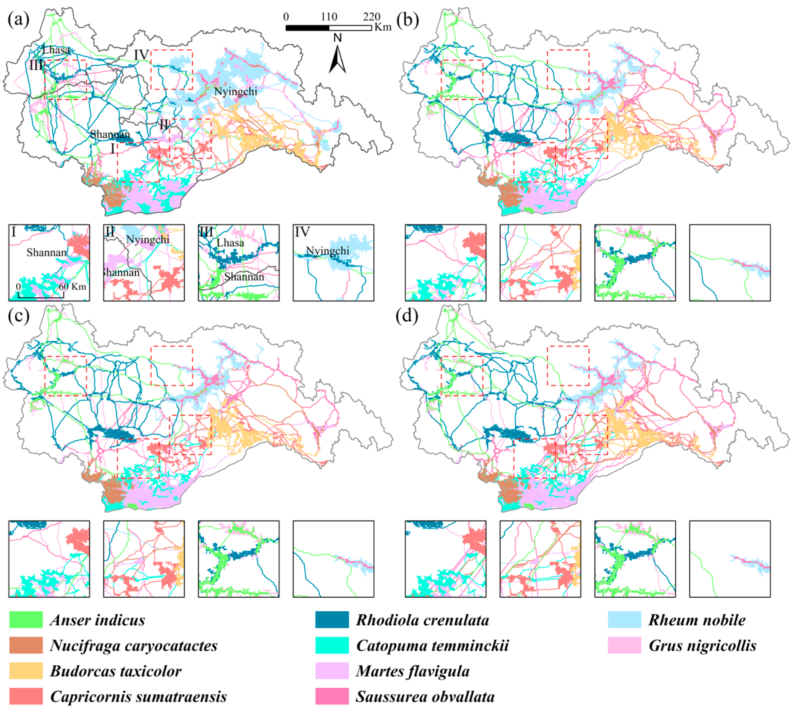
  • Changes in habitats and corridors: By 2030, the area of species’ habitats will have decreased by 12.9%, while the length of ecological corridors will have significantly increased under various scenarios. Changes in climate and LULC not only lead to a reduction in the area of suitable habitats for species but may also further increase the difficulty of species communication between habitats. Although the network topology indicators of the improvement scenario are better than those of the deterioration and baseline scenarios, there remains a significant difference compared to the baseline year of 1985.
  • Ecological protection planning: By optimizing the spatial layout of ecological elements, we propose a zoning and layout scheme of “two points, two cores, two belts, and two areas.” The regional hotspots are mainly located along corridors passing through areas of human activity and the edges of core habitats. This planning is based on the heterogeneity of the ecological space network and aims to enhance the connectivity of the HA-EN and the stability of species habitats.

Supplementary Materials

The following supporting information can be downloaded at: https://www.mdpi.com/article/10.3390/f15091506/s1, Figure S1: Environmental variable correlation; Figure S2: Spatial distribution of species and rivers in the study area; Table S1: Environment variable; Table S2: Definition of topological indicators. References [74,75] are cited in the Supplementary Materials.

Author Contributions

Conceptualization, C.L.; Methodology, C.L. and K.S.; Software, C.L.; Investigation, S.Y.; Resources, and X.J.; Writing—original draft, C.L.; Writing—review & editing, C.L., K.S. and and X.J.; Visualization, C.L.; Supervision, K.S. and S.Y.; Project administration, K.S. and S.Y.; Funding acquisition, K.S. and S.Y. All authors have read and agreed to the published version of the manuscript.

Funding

This research was funded by the Open Foundation of the State Key Laboratory of Urban and Regional Ecology of China (SKLURE2023-2-3), the Open Research Fund from the Key Laboratory of Forest Ecology in Tibet Plateau (Tibet Agricultural & Animal Husbandry University), Ministry of Education, China (XZA-JYBSYS-2023-09), and the Youth Science Foundation of the Natural Science Foundation of Guangxi (2022GXNSFBA035570).

Data Availability Statement

The original contributions presented in the study are included in the article and Supplementary Materials, further inquiries can be directed to the corresponding authors.

Acknowledgments

The authors are very grateful to the State Key Laboratory of Urban and Regional Ecology and researcher Wang Siyuan for their knowledge and technical guidance. We are also very grateful to the three anonymous reviewers for their valuable comments.

Conflicts of Interest

The authors declare no conflicts of interest.

References

  1. Heller, N.E.; Zavaleta, E.S. Biodiversity management in the face of climate change: A review of 22 years of recommendations. Biol. Conserv. 2009, 142, 14–32. [Google Scholar] [CrossRef]
  2. Scheffers, B.R.; De Meester, L.; Bridge, T.C.L.; Hoffmann, A.A.; Pandolfi, J.M.; Corlett, R.T.; Butchart, S.H.M.; Pearce-Kelly, P.; Kovacs, K.M.; Dudgeon, D.; et al. The broad footprint of climate change from genes to biomes to people. Science 2016, 354, aaf7671. [Google Scholar] [CrossRef] [PubMed]
  3. Xu, W.B.; Svenning, J.-C.; Chen, G.K.; Zhang, M.G.; Huang, J.H.; Chen, B.; Ordonez, A.; Ma, K.P. Human activities have opposing effects on distributions of narrow-ranged and widespread plant species in China. Proc. Natl. Acad. Sci. USA 2019, 116, 26674–26681. [Google Scholar] [CrossRef]
  4. Di Marco, M.; Santini, L. Human pressures predict species’ geographic range size better than biological traits. Glob. Chang. Biol. 2015, 21, 2169–2178. [Google Scholar] [CrossRef]
  5. Fei, S.L.; Desprez, J.M.; Potter, K.M.; Jo, I.; Knott, J.A.; Oswalt, C.M. Divergence of species responses to climate change. Sci. Adv. 2017, 3, e1603055. [Google Scholar] [CrossRef]
  6. Bay, R.A.; Harrigan, R.J.; Underwood, V.L.; Gibbs, H.L.; Smith, T.B.; Ruegg, K. Genomic signals of selection predict climate-driven population declines in a migratory bird. Science 2018, 359, 83–86. [Google Scholar] [CrossRef]
  7. Ceballos, G.; Ehrlich, P.R. Mammal Population Losses and the Extinction Crisis. Science 2002, 296, 904–907. [Google Scholar] [CrossRef]
  8. Bucciarelli, G.M.; Clark, M.A.; Delaney, K.S.; Riley, S.P.D.; Shaffer, H.B.; Fisher, R.N.; Honeycutt, R.L.; Kats, L.B. Amphibian responses in the aftermath of extreme climate events. Sci. Rep. 2020, 10, 3409. [Google Scholar] [CrossRef] [PubMed]
  9. Luedtke, J.A.; Chanson, J.; Neam, K.; Hobin, L.; Maciel, A.O.; Catenazzi, A.; Borzée, A. Ongoing declines for the world’s amphibians in the face of emerging threats. Nature 2023, 622, 308–314. [Google Scholar] [CrossRef] [PubMed]
  10. Liu, Y.C.; Li, Z.; Chen, Y.N. Continuous warming shift greening towards browning in the Southeast and Northwest High Mountain Asia. Sci. Rep. 2021, 11, 17920. [Google Scholar] [CrossRef]
  11. Yao, T.; Thompson, L.G.; Mosbrugger, V.; Zhang, F.; Ma, Y.; Luo, T.; Xu, B.; Yang, X.; Joswiak, D.R.; Wang, W.; et al. Third Pole Environment (TPE). Environ. Dev. 2012, 3, 52–64. [Google Scholar] [CrossRef]
  12. Qiu, J. China: The third pole. Nature 2008, 454, 393–396. [Google Scholar] [CrossRef]
  13. Fath, B.D.; Scharler, U.M.; Ulanowicz, R.E.; Hannon, B. Ecological network analysis: Network construction. Ecol. Model. 2007, 208, 49–55. [Google Scholar] [CrossRef]
  14. Hüse, B.; Szabó, S.; Deák, B.; Tóthmérész, B. Mapping an ecological network of green habitat patches and their role in maintaining urban biodiversity in and around Debrecen city (Eastern Hungary). Land Use Policy 2016, 57, 574–581. [Google Scholar] [CrossRef]
  15. Wang, S.; Wu, M.Q.; Hu, M.M.; Fan, C.; Wang, T.; Xia, B.C. Promoting landscape connectivity of highly urbanized area: An ecological network approach. Ecol. Indic. 2021, 125, 107487. [Google Scholar] [CrossRef]
  16. Verburg, P.H.; Schot, P.P.; Dijst, M.J.; Veldkamp, A. Land use change modelling: Current practice and research priorities. GeoJournal 2004, 61, 309–324. [Google Scholar] [CrossRef]
  17. Schulp, C.J.E.; Nabuurs, G.-J.; Verburg, P.H. Future carbon sequestration in Europe—Effects of land use change. Agric. Ecosyst. Environ. 2008, 127, 251–264. [Google Scholar] [CrossRef]
  18. Liu, X.; Liang, X.; Li, X.; Xu, X.; Ou, J.; Chen, Y.; Li, S.; Wang, S.; Pei, F. A future land use simulation model (FLUS) for simulating multiple land use scenarios by coupling human and natural effects. Landsc. Urban Plan. 2017, 168, 94–116. [Google Scholar] [CrossRef]
  19. Yin, H.W.; Kong, F.H.; Hu, Y.M. Assessing Growth Scenarios for Their Landscape Ecological Security Impact Using the SLEUTH Urban Growth Model. J. Urban Plan. Dev. 2016, 142, 05015006. [Google Scholar] [CrossRef]
  20. Fall, A.; Fortin, M.-J.; Manseau, M.; O’Brien, D. Spatial Graphs: Principles and Applications for Habitat Connectivity. Ecosystems 2007, 10, 448–461. [Google Scholar] [CrossRef]
  21. Urban, D.; Keitt, T. Landscape Connectivity: A Graph-Theoretic Perspective. Ecology 2001, 82, 1205–1218. [Google Scholar] [CrossRef]
  22. Jetz, W.; McGowan, J.; Rinnan, D.S.; Possingham, H.P.; Visconti, P.; O’Donnell, B.; Londoño-Murcia, M.C. Include biodiversity representation indicators in area-based conservation targets. Nat. Ecol. Evol. 2022, 6, 123–126. [Google Scholar] [CrossRef]
  23. Teng, M.; Wu, C.; Zhou, Z.; Lord, E.; Zheng, Z. Multipurpose greenway planning for changing cities: A framework integrating priorities and a least-cost path model. Landsc. Urban Plan. 2011, 103, 1–14. [Google Scholar] [CrossRef]
  24. Préau, C.; Grandjean, F.; Sellier, Y.; Gailledrat, M.; Bertrand, R.; Isselin-Nondedeu, F. Habitat patches for newts in the face of climate change: Local scale assessment combining niche modelling and graph theory. Sci. Rep. 2020, 10, 3570. [Google Scholar] [CrossRef]
  25. LaPoint, S.; Gallery, P.; Wikelski, M.; Kays, R. Animal behavior, cost-based corridor models, and real corridors. Landsc. Ecol. 2013, 28, 1615–1630. [Google Scholar] [CrossRef]
  26. Cushman, S.A.; Landguth, E.L.; Flather, C.H. Evaluating population connectivity for species of conservation concern in the American Great Plains. Biodivers. Conserv. 2013, 22, 2583–2605. [Google Scholar] [CrossRef]
  27. Bukvareva, E. The optimal biodiversity–A new dimension of landscape assessment. Ecol. Indic. 2018, 94, 6–11. [Google Scholar] [CrossRef]
  28. Taylor, P.D.; Fahrig, L.; Henein, K.; Merriam, G. Connectivity Is a Vital Element of Landscape Structure. Oikos 1993, 68, 571–573. [Google Scholar] [CrossRef]
  29. Tambosi, L.R.; Martensen, A.C.; Ribeiro, M.C.; Metzger, J.P. A Framework to Optimize Biodiversity Restoration Efforts Based on Habitat Amount and Landscape Connectivity. Restor. Ecol. 2014, 22, 169–177. [Google Scholar] [CrossRef]
  30. Hamonic, F.; Albert, C.; Couëtoux, B.; Vaxès, Y. Optimizing the ecological connectivity of landscapes. Networks 2023, 81, 278–293. [Google Scholar] [CrossRef]
  31. Pietsch, M. Contribution of connectivity metrics to the assessment of biodiversity—Some methodological considerations to improve landscape planning. Ecol. Indic. 2018, 94, 116–127. [Google Scholar] [CrossRef]
  32. Ricotta, C.; Stanisci, A.; Avena, G.C.; Blasi, C. Quantifying the network connectivity of landscape mosaics: A graph-theoretical approach. Community Ecol. 2000, 1, 89–94. [Google Scholar] [CrossRef]
  33. Saura, S.; Pascual-Hortal, L. A new habitat availability index to integrate connectivity in landscape conservation planning: Comparison with existing indices and application to a case study. Landsc. Urban Plan. 2007, 83, 91–103. [Google Scholar] [CrossRef]
  34. Keeley, A.T.H.; Ackerly, D.D.; Cameron, D.R.; Heller, N.E.; Huber, P.R.; Schloss, C.A.; Thorne, J.H.; Merenlender, A.M. New concepts, models, and assessments of climate-wise connectivity. Environ. Res. Lett. 2018, 13, 073002. [Google Scholar] [CrossRef]
  35. Bai, L.; Yao, Y.; Lei, X.; Liang, Z. Annual and Seasonal Variation Characteristics of Surface Temperature in the Qinghai–Tibetan Plateau. J. Geomat. 2018, 43, 15–18. [Google Scholar] [CrossRef]
  36. Luo, L.H.; Ma, W.; Zhuang, Y.L.; Zhang, Y.N.; Yi, S.H.; Xu, J.W.; Long, Y.P.; Ma, D.; Zhang, Z.Q. The impacts of climate change and human activities on alpine vegetation and permafrost in the Qinghai-Tibet Engineering Corridor. Ecol. Indic. 2018, 93, 24–35. [Google Scholar] [CrossRef]
  37. Dong, S.K. Revitalizing the grassland on the Qinghai–Tibetan Plateau. Grassl. Res. 2023, 2, 241–250. [Google Scholar] [CrossRef]
  38. Liang, X.; Liu, X.P.; Li, X.C.; Chen, Y.M.; Tian, H.; Yao, Y. Delineating multi-scenario urban growth boundaries with a CA-based FLUS model and morphological method. Landsc. Urban Plan. 2018, 177, 47–63. [Google Scholar] [CrossRef]
  39. Zhang, Y.; Zheng, M.R.; Qin, B. Optimization of spatial layout based on ESV-FLUS model from the perspective of “Production-Living-Ecological”: A case study of Wuhan City. Ecol. Model. 2023, 481, 110356. [Google Scholar] [CrossRef]
  40. Luo, H.Z.; Li, Y.Y.; Gao, X.Y.; Meng, X.Z.; Yang, X.H.; Yan, J.Y. Carbon emission prediction model of prefecture-level administrative region: A land-use-based case study of Xi’an city, China. Appl. Energy 2023, 348, 121488. [Google Scholar] [CrossRef]
  41. Wang, Q.Z.; Guan, Q.Y.; Sun, Y.F.; Du, Q.Q.; Xiao, X.; Luo, H.P.; Zhang, J.; Mi, J.M. Simulation of future land use/cover change (LUCC) in typical watersheds of arid regions under multiple scenarios. J. Environ. Manag. 2023, 335, 117543. [Google Scholar] [CrossRef] [PubMed]
  42. Jayanthi, M.; Duraisamy, M.; Thirumurthy, S.; Samynathan, M.; Muralidhar, M. Dynamics of land-use changes and their future trends using spatial analysis and the CA-Markov model—A case-study with a special emphasis on aquaculture development in India. Land Degrad. Dev. 2021, 32, 2563–2579. [Google Scholar] [CrossRef]
  43. Phillips, S.J.; Anderson, R.P.; Schapire, R.E. Maximum entropy modeling of species geographic distributions. Ecol. Model. 2006, 190, 231–259. [Google Scholar] [CrossRef]
  44. Qian, M.Y.; Huang, Y.T.; Cao, Y.R.; Wu, J.Y.; Xiong, Y.M. Ecological network construction and optimization in Guangzhou from the perspective of biodiversity conservation. J. Environ. Manag. 2023, 336, 117692. [Google Scholar] [CrossRef] [PubMed]
  45. Ortega-Andrade, H.M.; Prieto-Torres, D.A.; Gómez-Lora, I.; Lizcano, D.J. Ecological and Geographical Analysis of the Distribution of the Mountain Tapir (Tapirus pinchaque) in Ecuador: Importance of Protected Areas in Future Scenarios of Global Warming. PLoS ONE 2015, 10, e0121137. [Google Scholar] [CrossRef]
  46. Xu, C.L.; Yu, Q.; Wang, F.; Qiu, S.; Ai, M.S.; Zhao, J.K. Identifying and optimizing ecological spatial patterns based on the bird distribution in the Yellow River Basin, China. J. Environ. Manag. 2023, 348, 119293. [Google Scholar] [CrossRef]
  47. Jiang, H.; Peng, J.; Zhao, Y.N.; Xu, D.M.; Dong, J.Q. Zoning for ecosystem restoration based on ecological network in mountainous region. Ecol. Indic. 2022, 142, 109138. [Google Scholar] [CrossRef]
  48. Wang, L.Y.; Wang, S.Y.; Liang, X.F.; Jiang, X.B.; Wang, J.P.; Li, C.; Chang, S.H.; You, Y.F.; Su, K. How to Optimize High-Value GEP Areas to Identify Key Areas for Protection and Restoration: The Integration of Ecology and Complex Networks. Remote Sens. 2023, 15, 3420. [Google Scholar] [CrossRef]
  49. Li, C.; Su, K.; Liang, X.F. Identification of priority areas to provide insights for ecological protection planning: A case study in Hechi, China. Ecol. Indic. 2023, 154, 110738. [Google Scholar] [CrossRef]
  50. Chang, S.H.; Su, K.; Jiang, X.B. Impacts and Predictions of Urban Expansion on Habitat Connectivity Networks: A Multi-Scenario Simulation Approach. Forests 2023, 14, 2187. [Google Scholar] [CrossRef]
  51. Wang, Y.J.; Qu, Z.Y.; Zhong, Q.C.; Zhang, Q.P.; Zhang, L.; Zhang, R.; Yi, Y.; Zhang, G.L.; Li, X.C.; Liu, J.G. Delimitation of ecological corridors in a highly urbanizing region based on circuit theory and MSPA. Ecol. Indic. 2022, 142, 109258. [Google Scholar] [CrossRef]
  52. Wei, Q.Q.; Halike, A.; Yao, K.X.; Chen, L.M.; Balati, M. Construction and optimization of ecological security pattern in Ebinur Lake Basin based on MSPA-MCR models. Ecol. Indic. 2022, 138, 108857. [Google Scholar] [CrossRef]
  53. McRae, B.H. Isolation by Resistance. Evolution 2006, 60, 1551–1561. [Google Scholar] [CrossRef] [PubMed]
  54. McRae, B.H.; Beier, P. Circuit theory predicts gene flow in plant and animal populations. Proc. Natl. Acad. Sci. USA 2007, 104, 19885–19890. [Google Scholar] [CrossRef]
  55. Taylor, C.M.; Stutchbury, B.J.M. Effects of breeding versus winter habitat loss and fragmentation on the population dynamics of a migratory songbird. Ecol. Appl. 2016, 26, 424–437. [Google Scholar] [CrossRef]
  56. Xu, Y.; Si, Y.; Wang, Y.; Zhang, Y.; Prins, H.H.T.; Cao, L.; de Boer, W.F. Loss of functional connectivity in migration networks induces population decline in migratory birds. Ecol. Appl. 2019, 29, e01960. [Google Scholar] [CrossRef]
  57. Fan, Z. Simulation of land-cover change in Jing-Jin-Ji region under different scenarios of SSP-RCP. J. Geogr. Sci. 2022, 32, 421–440. [Google Scholar] [CrossRef]
  58. Shen, Z.; Wu, W.; Chen, S.; Tian, S.; Wang, J.; Li, L. A static and dynamic coupling approach for maintaining ecological networks connectivity in rapid urbanization contexts. J. Clean. Prod. 2022, 369, 133375. [Google Scholar] [CrossRef]
  59. Zeller, K.A.; Lewison, R.; Fletcher, R.J.; Tulbure, M.G.; Jennings, M.K. Understanding the Importance of Dynamic Landscape Connectivity. Land 2020, 9, 303. [Google Scholar] [CrossRef]
  60. Bishop-Taylor, R.; Tulbure, M.G.; Broich, M. Evaluating static and dynamic landscape connectivity modelling using a 25-year remote sensing time series. Landsc. Ecol. 2018, 33, 625–640. [Google Scholar] [CrossRef]
  61. Oliveira-Junior, N.D.d.; Heringer, G.; Bueno, M.L.; Pontara, V.; Meira-Neto, J.A.A. Prioritizing landscape connectivity of a tropical forest biodiversity hotspot in global change scenario. For. Ecol. Manag. 2020, 472, 118247. [Google Scholar] [CrossRef]
  62. Liu, T.; Chen, D.; Yang, L.; Meng, J.; Wang, Z.; Ludescher, J.; Fan, J.; Yang, S.; Chen, D.; Kurths, J.; et al. Teleconnections among tipping elements in the Earth system. Nat. Clim. Chang. 2023, 13, 67–74. [Google Scholar] [CrossRef]
  63. Wunderling, N.; Winkelmann, R.; Rockström, J.; Loriani, S.; Armstrong McKay, D.I.; Ritchie, P.D.L.; Sakschewski, B.; Donges, J.F. Global warming overshoots increase risks of climate tipping cascades in a network model. Nat. Clim. Chang. 2023, 13, 75–82. [Google Scholar] [CrossRef]
  64. Livina, V.N. Connected climate tipping elements. Nat. Clim. Chang. 2023, 13, 15–16. [Google Scholar] [CrossRef]
  65. Ren, L.; Huo, J.X.; Xiang, X.; Pan, Y.P.; Li, Y.Q.; Wang, Y.Y.; Meng, D.H.; Yu, C.; Chen, Y.; Xu, Z.C.; et al. Environmental conditions are the dominant factor influencing stability of terrestrial ecosystems on the Tibetan plateau. Commun. Earth Environ. 2023, 4, 196. [Google Scholar] [CrossRef]
  66. Feng, Z.; Li, X.; Hu, J.; Wang, L. Ecological security analysis of typical areas in the eastern Qinghai-Tibet Plateau based on landscape pattern. Chin. J. Ecol 2022, 41, 1188–1196. [Google Scholar]
  67. Han, D.L.; Huang, J.P.; Ding, L.; Zhang, G.L.; Liu, X.Y.; Li, C.Y.; Yang, F. Breaking the Ecosystem Balance Over the Tibetan Plateau. Earth’s Future 2022, 10, e2022EF002890. [Google Scholar] [CrossRef]
  68. IPCC. Climate Change 2013: The Physical Science Basis. Contribution of Working Group I to the Fifth Assessment Report of the Intergovernmental Panel on Climate Change 2013; IPCC: Geneva, Switzerland, 2013; 1535p. [Google Scholar]
  69. Jiao, K.; Gao, J.B.; Liu, Z.H. Precipitation Drives the NDVI Distribution on the Tibetan Plateau While High Warming Rates May Intensify Its Ecological Droughts. Remote Sens. 2021, 13, 1305. [Google Scholar] [CrossRef]
  70. Harris, R.B. Rangeland degradation on the Qinghai-Tibetan plateau: A review of the evidence of its magnitude and causes. J. Arid Environ. 2010, 74, 1–12. [Google Scholar] [CrossRef]
  71. Zhang, Q.; Ma, L.; Zhang, Z.H.; Xu, W.H.; Zhou, B.R.; Song, M.H.; Qiao, A.H.; Wang, F.; She, Y.D.; Yang, X.Y.; et al. Ecological restoration of degraded grassland in Qinghai-Tibet alpine region: Degradation status, restoration measures, effects and prospects. Acta Ecol. Sin. 2019, 39, 7441–7451. [Google Scholar]
  72. De Montis, A.; Caschili, S.; Mulas, M.; Modica, G.; Ganciu, A.; Bardi, A.; Ledda, A.; Dessena, L.; Laudari, L.; Fichera, C.R. Urban–rural ecological networks for landscape planning. Land Use Policy 2016, 50, 312–327. [Google Scholar] [CrossRef]
  73. De Montis, A.; Ganciu, A.; Cabras, M.; Bardi, A.; Peddio, V.; Caschili, S.; Massa, P.; Cocco, C.; Mulas, M. Resilient ecological networks: A comparative approach. Land Use Policy 2019, 89, 104207. [Google Scholar] [CrossRef]
  74. Yan, L.; Xi, W.J.; Zhang, Z.Y. Analysis of the Habitat Quality Changes and Influencing Factors in Chuxiong Prefecture under the Background of Landscape Pattern Changes. Int. J. Ecol. 2021, 10, 655–665. [Google Scholar] [CrossRef]
  75. Wang, B.X.; Cheng, W.M.; Lan, S.X. Impact of Land Use Changes on Habitat Quality in Altay Region. J. Resour. Ecol. 2021, 12, 715–728. [Google Scholar] [CrossRef]
Figure 1. Elevation and land use/land cover (LULC) of the study area.
Forests 15 01506 g001
Figure 2. Research framework. The research framework of this study is divided into three parts from top to bottom, including multi-scenario simulation of future LULC, construction of the ecological network, and analysis of the ecological network.
Forests 15 01506 g002
Figure 3. Spatial pattern change in LULC: (a) 1985 control network; (b) 2030 improvement network; (c) 2030 deterioration network; (d) 2030 baseline network and change transfer matrix of LULC; (e) 2030 improvement network; (f) 2030 deterioration network; (g) 2030 baseline network. (I) the intersection of high mountains and canyons, (II) dense forests, (III) urban neighborhoods, and (IV) grassland.
Forests 15 01506 g003
Figure 4. Spatial pattern of resistance surfaces in multi-scenario ecological networks: (a) 1985 control network; (b) 2030 improvement network; (c) 2030 deterioration network; (d) 2030 baseline network. The letters in the figure represent four typical regions, (I) the intersection of high mountains and canyons, (II) dense forests, (III) urban neighborhoods, and (IV) grassland.
Forests 15 01506 g004
Figure 5. The spatial distribution of networks. Each color represents a different species, patches represent ecological sources, and lines represent ecological corridors. (a) The 1985 control network; (b) 2030 improvement network; (c) 2030 deterioration network; (d) 2030 baseline network. The letters in the figure represent four typical regions, (I) the intersection of high mountains and canyons, (II) dense forests, (III) urban neighborhoods, and (IV) grassland.
Forests 15 01506 g005
Figure 6. Network topology for multi-scenario ecological networks.
Forests 15 01506 g006
Figure 7. A schematic diagram of the module division of the multi-species ecological network in the study area. Ecological sources with similar structure and close connection will form a module. The rectangle of each color represents a module, the lines in the rectangle represent different ecological sources, and the serial number of the source is marked at the bottom of the line. (a) The 1985 control network; (b) 2030 improvement network; (c) 2030 deterioration network; (d) 2030 baseline network.
Forests 15 01506 g007
Figure 8. Conservation patterns in the study area: (a) habitat for migratory birds; (b) grassland degradation and restoration areas; (c) rivers and canyons; (d) forest sea; (e) animals in captivity; (f) melting glaciers; (g) rocky desertification; (h) urban green space; (i) human-made development; (j) overgrazing. (Shot by Chuang Li).
Forests 15 01506 g008
Table 1. Data used in this study.
Data TypesIndicator FactorsYearsData Sources
Climatic variables19 bioclimates (see Table S1 for details)1970–2000 and 2021–2040http://www.worldclim.org
(accessed on 1 January 2024)
Geographical dataElevation2020https://www.resdc.cn/
(accessed on 1 January 2024)
LULC1985, 2000, 2015, and 2020https://data.casearth.cn/
(accessed on 1 January 2024)
NDVI2020https://www.resdc.cn/
(accessed on 1 January 2024)
Soil type2020https://www.resdc.cn/
(accessed on 1 January 2024)
Vegetation type2020https://www.resdc.cn/
(accessed on 1 January 2024)
Road2020https://www.openstreetmap.org
(accessed on 1 January 2024)
Water2020https://www.resdc.cn/
(accessed on 1 January 2024)
Socio-economic dataGross domestic product2020http://www.resdc.cn/
(accessed on 1 January 2024)
Population density2020http://www.resdc.cn/
(accessed on 1 January 2024)
Settlement data2020http://www.resdc.cn/
(accessed on 1 January 2024)
Table 2. Resistance factor grading and weight.
Resistance FactorResistance Factor AssignmentWeight
15102050
Elevation/m≤1500(1500–3000](3000–4000](4000–5000]>50000.04
Water distance/km≤1(1–3](3–5](5–7]>70.15
Road distance/km>20(10–20](5–10](1–5]≤10.05
NDVI(0.7–1](0.5–0.7](0.3–0.5](0.1–0.3]≤0.10.11
Habitat provision(80–100](60–80](40–60](40–20](20–0]0.14
LULCForest, wetlandsGrasslandWater, croplandUnused landImpervious surface0.5
Table 3. Changes in network values for networks.
ParametersControl
Network
Improvement
Network
Deterioration
Network
Baseline
Network
Area of ecological sources/km2
(overlapping rate of source areas)
71,891.3 (25.4%)62,629.3 (30.8%)
Number of ecological sources180167167167
Number of ecological corridors346345343343
Average length of ecological corridors/m62,589.364,669.065,213.364,990.9
Average resistance value of corridors8.610.210.49.8
Intersection point of ecological corridors555485490506
Intersection point of ecological corridors/area of ecological sources0.007720.007740.007820.00808
Table 4. Conservation pattern and countermeasures.
PatternContentDefinitionCountermeasure
Two pointsBreak point and stepping stoneThe break point is the intersection of the animal corridor and the road; a stepping stone is the intersection of two roads and a corridor.Building an animal corridor at the break point; the stepping stone area restricts human activities.
Two coresGrassland degradation areaThe most obvious area of grassland degradation.Strictly restrict grazing, return farmland to grassland, study the degradation mechanism of alpine grassland, and find a breakthrough plan.
Two beltsCorridor core zoneThe strip area with the highest corridor density.Restrict the discharge of construction and pollution sources and establish protection countermeasures according to the migration date and habits of animals.
Two zonesRestoration areas and conservation areasComparing the ecological sources in 1985 and 2030, the lost ecological source in 2030 is the restoration area, and the emerging ecological source is the conservation area.The conservation and restoration countermeasures shall be formulated by zoning, and the countermeasures for the first ecological resistance source in the restoration area shall be studied, so as to prevent the degradation and fragmentation of the conservation area.
Disclaimer/Publisher’s Note: The statements, opinions and data contained in all publications are solely those of the individual author(s) and contributor(s) and not of MDPI and/or the editor(s). MDPI and/or the editor(s) disclaim responsibility for any injury to people or property resulting from any ideas, methods, instructions or products referred to in the content.

