Article

EIAGA-S: Rapid Mapping of Mangroves Using Geospatial Data without Ground Truth Samples

School of Information Science and Technology, Hainan Normal University, Haikou 571158, China
*
Author to whom correspondence should be addressed.
Forests 2024, 15(9), 1512; https://doi.org/10.3390/f15091512 (registering DOI)
Submission received: 26 July 2024 / Revised: 24 August 2024 / Accepted: 26 August 2024 / Published: 29 August 2024
(This article belongs to the Special Issue New Tools for Forest Science)

Abstract

:
Mangrove forests are essential for coastal protection and carbon sequestration, yet accurately mapping their distribution remains challenging due to spectral similarities with other vegetation. This study introduces a novel unsupervised learning method, the Elite Individual Adaptive Genetic Algorithm-Semantic Inference (EIAGA-S), designed for the high-precision semantic segmentation of mangrove forests using remote sensing images without the need for ground truth samples. EIAGA-S integrates an adaptive Genetic Algorithm with an elite individual’s evolution strategy, optimizing the segmentation process. A new Mangrove Enhanced Vegetation Index (MEVI) was developed to better distinguish mangroves from other vegetation types within the spectral feature space. EIAGA-S constructs segmentation rules through iterative rule stacking and enhances boundary information using connected component analysis. The method was evaluated using a multi-source remote sensing dataset covering the Hainan Dongzhai Port Mangrove Nature Reserve in China. The experimental results demonstrate that EIAGA-S achieves a superior overall mIoU (mean intersection over union) of 0.92 and an F1 score of 0.923, outperforming traditional models such as K-means and SVM (Support Vector Machine). A detailed boundary analysis confirms EIAGA-S’s ability to extract fine-grained mangrove patches. The segmentation includes five categories: mangrove canopy, other terrestrial vegetation, buildings and streets, bare land, and water bodies. The proposed EIAGA-S model offers a precise and data-efficient solution for mangrove semantic mapping while eliminating the dependency on extensive field sampling and labeled data. Additionally, the MEVI index facilitates large-scale mangrove monitoring. In future work, EIAGA-S can be integrated with long-term remote sensing data to analyze mangrove forest dynamics under climate change conditions. This innovative approach has potential applications in rapid forest change detection, environmental protection, and beyond.

1. Introduction

Mangroves are among the most productive ecosystems, and they are mainly distributed in the intertidal zones of tropical and subtropical areas, with tremendous social, ecological, and economic value [1,2]. However, influenced by human activities and other factors, mangrove ecosystems are under serious threat [3,4]. Remote sensing technology plays a critical role in mangrove monitoring [5,6]. Furthermore, the semantic segmentation of mangroves is a prerequisite for studies on mangrove change monitoring, area estimation, risk warning, etc. [7]. Therefore, the accurate extraction of semantic information from images is of great importance [8]. However, mangrove segmentation is affected by image classification techniques and sensor resolutions [9,10,11]. In addition, mangroves have similar spectral characteristics to other forms of vegetation, croplands, and analogous objects [12,13]. Meanwhile, the limited scale of mangrove datasets and segmentation accuracy has long been a bottleneck in remote sensing image semantic segmentation [14,15].
Earlier remote sensing image semantics relied on human cognition and understanding to set parameters [16]. Manually setting feature extraction parameters for remote sensing images is extremely difficult [17,18,19,20]. Given the advancements in deep learning and machine learning technologies, numerous high-performance semantic segmentation networks have been developed [21,22,23,24]. Chen et al. [25] introduced an improved semantic segmentation framework, SDFCNv2, based on SDFCNv1, and devised a post-processing algorithm for the segmentation of ultra-large remote sensing images using mask-weighted voting decisions. This enhancement led to an increase of up to 5.22% in the mIoU metric. Guo et al. [26] proposed the ME-Net semantic segmentation model based on the Fully Convolutional Network (FCN) architecture to dynamically delineate and monitor mangrove forest distribution areas. With the global attention module, multi-scale context embedding, and boundary fitting unit, the overall accuracy of the extraction network reached 97.48%. Fu et al. [27] integrated recursive feature elimination (RFE) and deep learning (DL) algorithms to stack five foundational models (Random Forest, XGBoost, LightGBM, CatBoost, and AdaBoost) to construct an ensemble learning model (SEL), achieving an overall accuracy of 94.8%. Sun et al. [28] developed a detailed mangrove mapping method for long-term time series data using five sensor types and a U-Net model, achieving an average accuracy of 92.54% for mangrove extraction. This supports sustainable mangrove ecosystem management.
However, neural networks are often regarded as black boxes, and network training relies on a large number of parameters, resulting in the considerable loss of semantic information. This makes it difficult to explain their internal workings and decision processes [29]. In addition, deep learning and machine learning models heavily depend on large amounts of training data, requiring substantial computational resources [30,31,32]. Additionally, methods using convolutional modules often struggle with decision-making in complex semantic areas, such as class boundaries, small patches, and mixed pixels [32,33]. While high-resolution data can significantly alleviate this issue, obtaining and annotating such data is challenging [33,34].
Swarm intelligence algorithms offer innovative solutions for applications across various fields and continue to undergo enhancements [35,36,37]. Numerous researchers have explored the applications of swarm intelligence algorithms, achieving significant results [38,39]. To alleviate the need for extensive field sampling in remote sensing research while addressing the challenges posed by the variability and instability of data collection equipment, in this article, we introduce a swarm intelligence algorithm into the mapping of mangrove forests. We propose an Elite Individual Adaptive Genetic Algorithm for Semantic Segmentation Model (EIAGA-S), which enables the rapid mapping of mangrove growth areas without the need for ground truth samples. The EIAGA-S algorithm enhances the traditional adaptive Genetic Algorithm by modifying the genetic and mutation strategies of the conventional GA and incorporating an elite individual evolution strategy. This optimizes the slow convergence issues and susceptibility to local optima typically associated with traditional genetic algorithms. Furthermore, the OTSU algorithm is employed as the objective optimization function, replacing the manual threshold adjustments commonly used in mangrove extraction and facilitating dynamic parameter adjustments for data collected under various sensor and lighting conditions. Additionally, to enhance the distinguishability of mangrove features, in this study, we employ a Modified Enhanced Vegetation Index (MEVI) specifically tailored for mangroves, improving the discrimination between mangroves and other types of vegetation. In the final stage, EIAGA-S utilizes a tree-based decision reasoning method to construct semantic decision rules, classifying objects into five categories: mangrove canopies, water bodies, land, other terrestrial vegetation, and buildings.
The primary contributions of this study are as follows:
(1)
Stable and unsupervised segmentation: The EIAGA-S model eliminates the need for extensive field sampling and labeled data, achieving stable and accurate mapping results without relying on ground truth samples. This makes it a practical and efficient solution for large-scale mangrove monitoring.
(2)
Boundary and small object segmentation: The EIAGA-S model excels in boundary delineation and small object segmentation. It accurately identifies fine details such as small river tributaries and complex terrain features, outperforming other methods like GA, K-means, SVM, and U-Net in handling intricate and dispersed objects.
(3)
The development and application of MEVI: A new Mangrove Enhanced Vegetation Index (MEVI) was developed to better distinguish mangroves from other vegetation types. This index improves the discrimination within the spectral feature space, enhancing the overall segmentation accuracy and supporting effective monitoring in areas like the Hainan Dongzhai Port Mangrove Nature Reserve.

2. Materials

The research area, an integral part of the Dongzhai Port Nature Reserve, is strategically located at the intersection of Haikou City and Wenchang City in the northeastern part of Hainan Province, China (Figure 1). The geographical coordinates of this area range from 110°32′ to 110°37′ E in longitude and 19°51′ to 20°1′ N in latitude. The area experiences a stable annual average temperature of approximately 23.8 °C. It spans a total of 3337.6 hectares, with the core zone accounting for 1635 hectares. The mangrove coverage, extending over a significant area of 1771 hectares, coexists harmoniously with the coast-line, spanning a length of 28 km. This region is home to the largest, most diverse, and best-preserved mangrove forest in China. It hosts five families and eight genera of mangroves, comprising eleven species [26].
On 4 May 2024, a survey was conducted in the study area using the MATRICE 350 RTK hexacopter (DJI Technology Co., Ltd. (Shenzhen, China)), equipped with GNSS (global navigation satellite system) receivers for the RTK (real-time kinematic) method, achieving a horizontal position accuracy of 1 cm + 1 ppm and a vertical accuracy of 1.05 cm + 1 ppm. This UAV carried a DJI Mavic 3E, capturing high-resolution orthoimagery with a resolution of 20 million pixels. The UAV flew at an altitude of 115 m, meeting a 1:500 precision requirement, with a longitudinal overlap of 75% and a lateral overlap of 80%. Stable wind conditions ensured optimal performance. The survey area spanned coordinates from 20°1′7″ N to 19°57′46″ N and 110°32′4″ E to 110°34′41″ E. During the survey, the tide was notably low, exposing most mangrove stands in the intertidal zone, allowing for the identification of fine-scale mangrove patches. Field surveys took place on 12–14 December 2023 and 4–5 May 2024, in the Dongzhai Port study area, to verify the mangrove patch boundaries and assess the growth of newly established mangroves. Combining ground-based observations with orthoimagery from UAVs enabled precise delineation of mangrove forest growth boundaries.
In this study, we utilized satellite imagery from three distinct sources: WorldView-2, with a spectral resolution of 0.4 m, Sentinel-2, with 20 m, and Landsat 8, with 30 m. The remote sensing data from all three satellite sources underwent radiometric calibration to ensure accuracy. The WorldView-2 offers higher resolution, resulting in less mixed pixel imagery. In contrast, Sentinel-2 and Landsat 8 satellites have relatively low resolutions.

3. Methodology

Figure 2 illustrates the main process of EIAGA-S. The raw band information and vegetation indices provide the data foundation. Next, the Building module of EIAGA-S offers the optimal thresholds for class division. Subsequently, the Decision module of EIAGA-S performs semantic fusion decision-making.

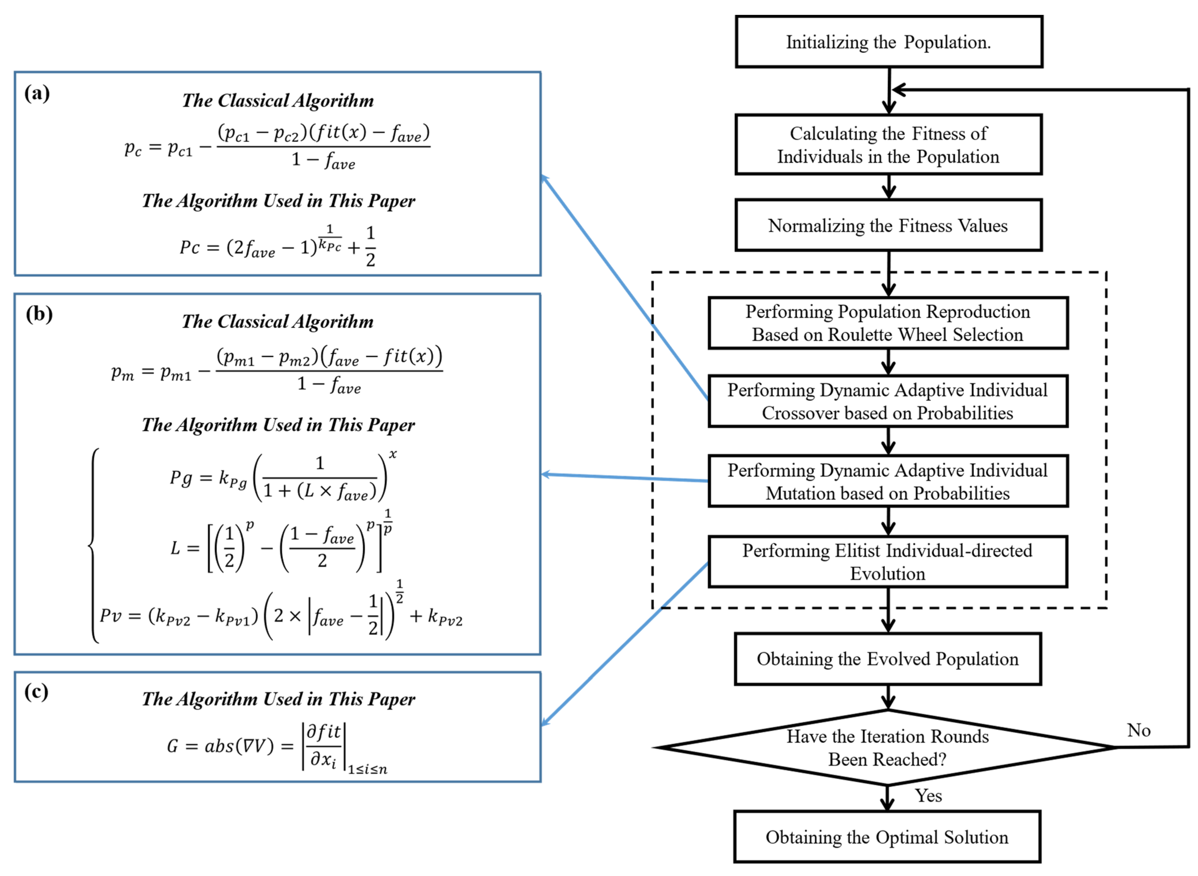
3.1. Elite Individual Adaptive Genetic Algorithm

Based on the population’s average fitness, EIAGA-S resets the “crossover” and “mutation” operators and employs elite individuals to guide the population’s evolutionary direction. The flowchart of EIAGA-S is depicted in Figure 3.

3.1.1. Population Encoding and Fitness Function

In this study, assuming that the remote sensing data need to be divided into c classes, c − 1 threshold variables need to be set within the range [0, 255]. A set of segmentation threshold variables H can be denoted as {0, k1, k2, ⋯, kc−1, 255}. Using an 8-bit binary code (i.e., 2 8 = 256 possible threshold values) to represent a segmentation threshold, a population individual x can be represented by an 8 × (c − 1) bit code. The OTSU algorithm is selected as the fitness function for optimizing individual encoding [40,41]. The function f(x) represents the fitness value of individual x for the target problem. A higher fitness value f(x) indicates better genetic encoding of individual x, suggesting improved optimization results for the population.
The normalization of fitness values provides an intuitive representation of the distribution of individual fitness within the population. The calculation method is given by Equation (1):
fit ( x ) = f ( x ) f min f max f min
where f(x) represents the fitness of an individual, fmax represents the maximum normalized fitness value within the population, and fmin represents the minimum normalized fitness value within the population. The resulting values fit(x) are distributed within the range of [0, 1].

3.1.2. Adaptive Crossover and Mutation Strategies

In the early stages, the adaptation of the population is dispersed. As iterations progress, the population gradually converges. However, convergence does not necessarily mean optimality. Therefore, EIAGA-S introduces the average fitness (Equation (2)):
f ave = i = 1 n fit ( x i ) n
where fave represents the average fitness, and n is the size of the population. If fit(xi) exceeds fave, it is considered an elite individual. Therefore, when fave is closer to fmax, this indicates that the average fitness of individuals in the population is higher and that the proportion of elite individuals is larger.
Population crossover (Pc) exchanges genes between individuals in a population to produce new individuals. In the past, researchers proposed various methods of Pc. Studies have indicated that uniform crossover is an efficient method for Pc [42,43]. Building on this, EIAGA-S uses fave to dynamically regulate the iteration process, as shown in Equation (3):
Pc ( x ) = ( 2 f ave 1 ) 1 k Pc + 1 2         k Pc = 2 m + 1 ( m 1 )
Here, kpc = 9 was determined experimentally. In this setting, when the population contains many elite individuals, Pc(x) increases to obtain better individuals. Conversely, when elite individuals are scarce, the Pc(x) probability decreases, and the mutation rate increases to explore more promising evolutionary directions.
The mutation module improves solutions by altering individual genes. However, excessive mutation can disrupt optimal solutions, while when there is too little mutation, it is difficult to escape local optima. Therefore, EIAGA-S sets a population mutation rate (Pm) and a gene mutation rate (Gm). P determines which individuals in the population undergo mutation, and Gm decides which genes within an individual are mutated. Generally, Gm is inversely proportional to fitness. Thus, Gm is set as shown in Equation (4).
Gm ( x ) = k Gm ( 1 1 + L × f ave ) x
where kGm = 0.22 is used to control the upper limit of the Gm(x), and L is the offset operator, which increases the change gradient of the Gm for individuals with low fitness and decreases it for individuals with higher fitness. The calculation method is as follows, in Equation (5):
L = [ ( 1 2 ) p ( 1 f ave 2 ) p ] 1 p
where p = 2. When fave is low, the L operator further reduces Gm. As fave increases, Gm is moderately lowered to prevent excessive interference with the solution. Additionally, to avoid premature convergence, a lower limit for Gm is set.
In classical GA, the value of Pm is fixed; however, a fixed Pm may not be suitable for all populations. EIAGA-S believes that populations with fewer elite individuals require a larger Pm to explore better evolutionary directions, while populations with more elite individuals also require a larger Pm to prevent excessive accumulation. Therefore, when fave is either low or high, a larger Pm need to be set, as shown in Equation (6):
Pm ( x ) = ( k Pm2 k Pm1 ) ( 2 × | f ave 1 2 | ) 1 2 + k Pm1
where kPm1 and kPm2 are control parameters for upper and lower limits, kPm1 is the lower limit of the mutation rate for the Pm operator, with a value of 0.2, while kPm2 is the upper limit of the mutation rate for the Pm operator, with a value of 0.28. The Pm is uniformly distributed between sets [kPm1, kPm2].

3.1.3. Elite-Individual-Oriented Evolutionary Strategy

Elite individuals can act as a “compass”. Based on this, EIAGA-S establishes a directional evolution strategy. Assuming that the optimization problem involves n dimensions, the fitness equation of the best individual is represented as f i t x 1 , , x n , where x1, x2, …, xn are the n dimensions of the optimization problem. Thus, the potential optimization direction can be represented by Equation (7):
V = [ fit ( ( x 1 + λ e ) , x 2 L , x n ) fit ( x 1 , ( x 2 + λ e ) L , x n ) fit ( x 1 , x 2 L , ( x n + λ e ) ) ]
where V represents the set of individual evolution directions. In remote sensing image segmentation tasks, the continuity of the optimization problem addressed by EIAGA-S is not known. Therefore, the minimum unit length of individual encoding is treated as a unit vector, obtaining the growth gradient of elite individuals, as shown in Equation (8):
fit x i = lim Δ x 0 fit ( x 1 , , ( x i + Δ x i ) , , x n ) fit ( x 1 , , x i , , x n ) Δ x i fit ( x 1 , , ( x i + λ e ) , , x n ) fit ( x 1 , , x i , , x n ) e
Therefore, the evolutionary gradient values for the best individual in all directions are obtained as follows:
G = abs ( V ) = | fit x i | 1 i n
It is important to note that if the target problem has multiple evolutionary directions, the population size may need to be increased or filtered. Otherwise, the algorithm is more likely to become trapped in a local optimum, affecting the final result.

3.2. Semantic Information Enhancement Method for Mangrove (MEVI)

Mangroves have two unique characteristics compared to typical vegetation. Firstly, they have dense canopy growth with stable spectral features. Secondly, they grow in the inter-tidal zone, where although the water’s strong absorption in the infrared band creates differences from terrestrial vegetation, they also remain distinct from submerged vegetation.
Vegetation indices are widely used to analyze vegetation growth, species distribution, and related areas [44,45,46,47,48]. Normalized Difference Vegetation Index (NDVI) [49], LSWI [50,51], MNDVI [52], and others provide critical information and are commonly used in tidal vegetation monitoring, as shown in Equations (10)–(12):
NDVI = ( NIR R ) ( NIR + R )
LSWI = ( NIR SWIR ) ( NIR + SWIR )
MNDWI = ( G SWIR ) ( G + SWIR )
where R represents the red band, NIR represents the near-infrared band, and SWIR represents the short-wave infrared band. To better distinguish mangroves from other tree species, their unique characteristics in wetland ecosystems are considered. The NIR2 influence coefficient is introduced to develop the Mangrove Enhanced Vegetation Index (MEVI), as shown in Equation (13):
MEVI = ( ρ 705 ρ 665 ) ε ρ 1610
where ε = 0.4 is an empirical parameter, with its optimal value determined through experimental tuning. In the near-infrared band, vegetation reflectance gradually increases, peaking around 1.1 μm. The reflectance in the red-edge region depends on the internal chlorophyll content. The rate of increase in reflectance of mangroves in the red-edge band differs from other vegetation. ρ705 − ρ665 captures this change [53]. However, this result has some fluctuations, as the chlorophyll content in mangroves is unstable under different growth and density conditions [54]. Additionally, the ρ1610 band helps to collect additional information about water content fluctuations [55,56]. Due to the unique growing environment of mangroves in intertidal zones, the water content in mangrove growing areas is far greater than in general terrestrial vegetation growing areas.
The combination in MEVI highlights the differences between mangroves and other terrestrial vegetation, as well as the differences between mangrove growing environments and other vegetation growing environments. Therefore, it effectively enhances the characteristics of mangroves. The setting of ε is aimed at fluctuations in different study areas, dynamically setting a more effective combination factor for this combination.

3.3. Semantic Feature Decision

3.3.1. Connectivity Analysis

Mangrove areas with poor growth and boundary regions often blend with other categories, creating mixed pixels in lower-resolution data, leading to spectral instability. The introduction of connectivity analysis is designed to eliminate uncertainty in decision-making.
Assume that an open set G exists on a 2D image. If any closed curve within G always belongs to G, it is called a simply connected domain. In image processing, searching for connected domains includes 4-connectivity and 8-connectivity. The 8-connectivity growth pattern typically produces larger connected components. In this study, we chose the 8-connectivity growth pattern, using an image segmentation module to process coastal images, extract mangrove areas from segmentation results, calculate the connected area, and remove connected regions smaller than 0.05.
Connectivity analysis reduces the impact of mixed pixels on final decisions, enhances mangrove flux information, and improves the accuracy of semantic analysis.

3.3.2. Classification Decision

Different objects exhibit distinct characteristics across various spectral bands. Therefore, EIAGA-S integrates different semantics for effective classification. Thanks to improvements in its internal structure, the optimization results are stable, replacing the manual threshold-setting process. For different segmentation tasks, only the segmentation parameters need to be reset based on collected data and specific segmentation goals.
In remote sensing images, since chlorophyll and other pigments in plant cells absorb more visible light, the low band radiation in C, B, G, Y, and R is usually reflected by vegetation cells and chlorophyll structures, exhibiting higher reflectivity and a darker color. The absorption rates of RE, NIR1, and NIR2 are higher, presenting brighter colors. On the contrary, molecules and suspended substances in water can absorb or scatter radiation in high-wavelength bands, with higher radiation absorption rates in the RE, NIR1, and NIR2 bands. Therefore, information on water bodies, such as oceans, rivers, and pools, exhibits distinct information characteristics in the RE, NIR1, and NIR2 bands. Especially for a semantic understanding of land–water information in conditions of poor mobility and the growth of algae and microorganisms, high-band spectral data can provide a more accurate and effective understanding.
The absorption rate of semantic information on objects such as houses, residential areas, and streets for low-wavelength spectra is low, so the target semantics have obvious semantic features in the C, B, G, Y, and R bands, and the image is brighter. However, in the RE and NIR1 bands, there are similar characteristics for certain land information, with sparse plants. Due to the complexity of the land situation, its semantic features are unstable in the range of approximately 585 nm–745 nm under different water contents and vegetation coverages. The spectral information under the high-wavelength radiation of 745 nm–1040 nm has similar characteristics to the semantics of vegetation with higher chlorophyll content. The semantic information within this band is less affected by the categories of land, trees, and grass, and can obtain more accurate semantic analysis results for house and street categories.
Assume that a certain input pixel in the image is x, and that the semantic information of x is as follows: in the coastal band, xC, blue band, xB, green band, xG, yellow line band, xY, red band, xR, near-infrared band 2, xNIR2 and xMEVI. Perform connectivity analysis on the xR band to obtain xCAR. We obtain the final segmentation results using the following approach:
R 1 : I f ( x CAR i s T u r e ) t h e n y i s m a n g r o v e s R 2 : I f ( x CAR i s F a l s e ) ( x NIR2 i s T r u e ) t h e n y i s w a t e r R 3 : I f ( x CAR i s F a l s e ) ( x NIR2 i s F a l s e ) ( x Y i s T r u e ) t h e n y i s h o u s e R 4 : I f ( x CAR i s F a l s e ) ( x NIR2 i s F a l s e ) ( x Y i s F a l s e ) ( x MEVI i s T r u e ) t h e n y s h r u b s R 5 : I f ( x CAR i s F a l s e ) ( x NIR2 i s F a l s e ) ( x Y i s F a l s e ) ( x MEVI i s F a l s e ) t h e n y l a n d

3.4. Experimental Evaluation Indicators

Mean intersection over union (mIoU) and F1 score are selected as two evaluation indicators to evaluate the segmentation effect of the segmentation model in this article. The mathematical expression of IoU is shown in Equation (14) [57]:
IoU = U 1 U 2 U 1 U 2
Assuming that pixels are divided into n classes in semantic segmentation, the calculation method for mIoU is as follows:
mIoU = i = 0 n IoU i n
The higher the mIoU value, the better the segmentation effect of the model.
The F1 score is a metric that combines precision and recall to provide a single score that balances both. F1 score is shown in Equation (16) [58]:
F 1 = 2 × Precision × Recall Precision + Recall

4. Experimental Results and Analysis

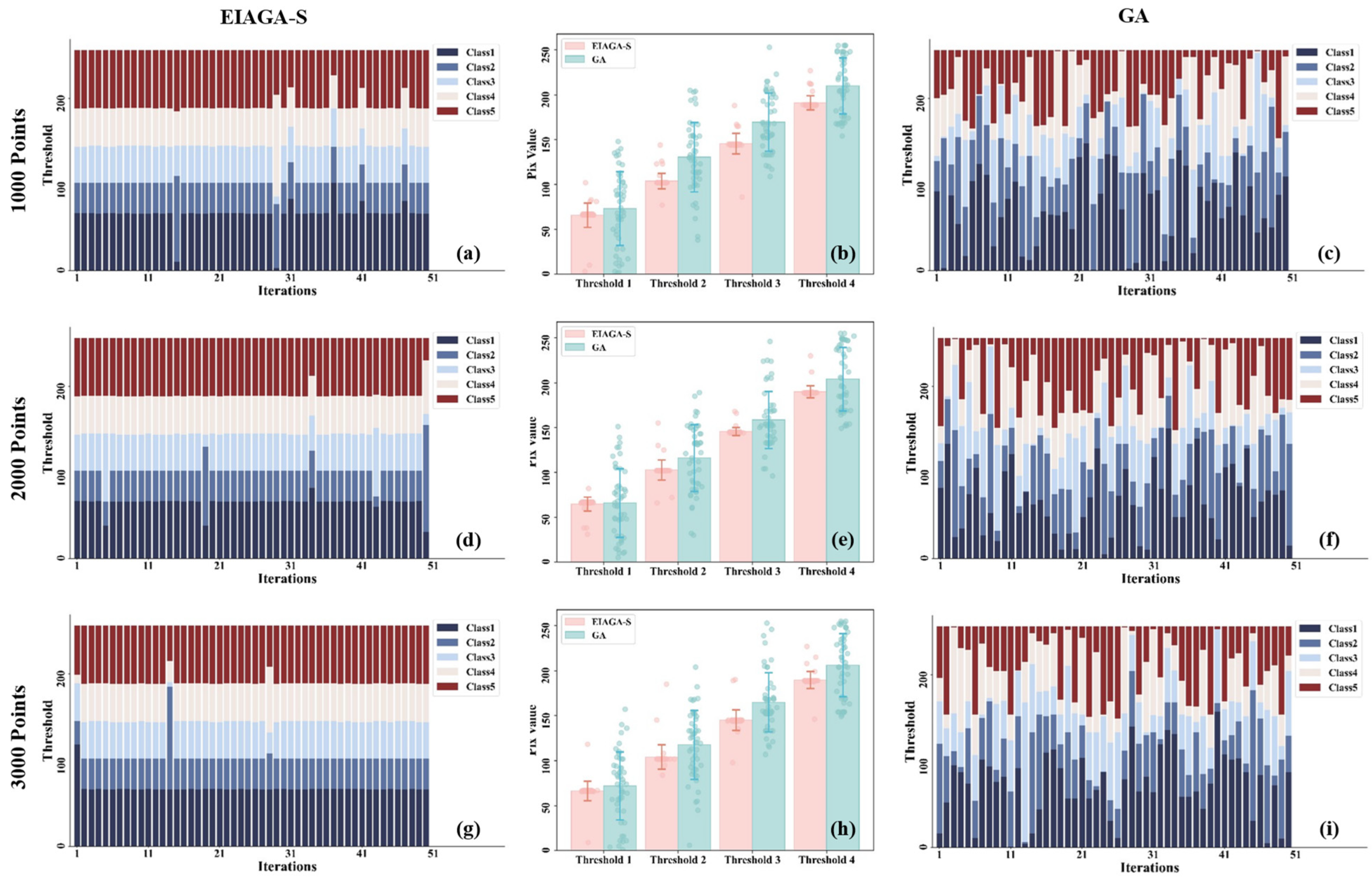
4.1. Precision and Result Analysis of EIAGA-S

To validate the advantages of EIAGA-S in complex semantic segmentation tasks involving remote sensing images, a comparative analysis was conducted with GA, K-means, SVM algorithms, and U-net network. All the algorithms were set with the same classification number, and the input band features were identical (B, G, R, NIR1, NIR2). K-means was implemented with default parameter settings. The SVM performed spatial random sampling from the training set, collecting spectral features of 1000 points with classification labels for training. The U-net network, requiring a larger training sample, divided the original image into 58 feature matrices of 200 × 200, and training was conducted with a 1:1 split of the training set and validation set over 200 iterations. The experiments were conducted on a Windows 11 system. The primary hardware included a 2.20 GHz 6-core i7-8750H CPU, 24 GB of RAM, and an NVIDIA GTX 1050 Ti GPU. The image processing, machine learning, and deep learning modules were developed using Python 3.11. The key libraries included OpenCV 4.9.0, sklearn 1.4.1, and PyTorch 2.2.1, with CUDA 11.8 support. The semantic segmentation classes in the experiment consisted of five categories, mangroves, shrubs (other vegetation), buildings, land, and ocean, totaling 2,147,961 segmentation pixels. The pixel category labels were determined based on UAV and field data.
The statistics for the semantic segmentation results for each algorithm were obtained from experiments conducted on WorldView-2 data. The mIoU values for the predicted category information were calculated, as shown in Table 1.
The F1 score values for all the predicted pixels in each category were calculated and presented in Table 2.
According to the evaluation data from Table 1 and Table 2, except for the GA, all the algorithms demonstrated favorable segmentation results for mangroves, with the EIAGA-S algorithm achieving the highest processing accuracy. Furthermore, for all the segmentation targets, EIAGA-S consistently attained optimal segmentation precision. The comparison between EIAGA-S and GA serves to validate the effectiveness of the improvement on GA. Additionally, the comparison with K-means highlights the limitations of general unsupervised segmentation algorithms in accurately capturing image semantics.
K-means, the U-Net network, and our proposed algorithm all achieved good results in predicting samples for the mangrove and ocean categories with relatively concentrated distribution areas. The U-Net network and our proposed algorithm have more advantages in ocean recognition. However, for intertidal flats, shrubs, and residential areas with dispersed distribution and complex features, the segmentation results of various comparison algorithms were poor. Due to the complex surface information features of intertidal flats, shallow machine learning algorithms such as SVM, GA, and K-means were unable to accurately capture sample rules, and they were often misclassified as other categories, with mIoU values below 10%. The U-Net neural network was able to extract higher-dimension features through multi-layer convolutional layers, which improved the detection effect to a certain extent, but the mIoU value was still only 27%. Our proposed algorithm further improved the results by incorporating vegetation index and connectivity density analysis based on multi-band data. The F1 score reached 76%, and the mIoU reached 61%.
In terms of the shrub category, due to the similarity of its features to those of mangroves, the GA algorithm and SVM algorithm showed poor performance in terms of the mIoU and F1 score. The K-means algorithm and U-Net network had better segmentation results, with the F1 score evaluation results reaching above 60%.
The residential area category has more distinct image features, but it often accounts for a relatively small proportion of remote sensing images. Therefore, the U-Net network and SVM algorithm had poor detection effects on residential areas due to the loss of high-dimensional features during the classification and extraction. Compared to the analysis of global features, the GA algorithm and K-means algorithm extracted more residential area information, resulting in some improvements in the F1 score and mIoU, but still with results of less than 50%. The proposed algorithm extracted features based on multi-dimensional characteristics, achieving a detection mIoU of 90% for this category, a significant improvement.
Utilizing the EIAGA-S model, an estimation was conducted within the research area located between the northeastern part of Dongzhaigang and the northwestern part of Wenchang city. The mangrove area was approximately 634.59 hectares. This research area is a part of the Dongzhaigang Mangrove Reserve in Haikou City, Hainan Province, China. The estimated area has a similar ratio compared to the total area of the reserve (based on the calculation data published by the National Forestry and Grassland Administration and National Park Administration of China (https://www.forestry.gov.cn/c/www/sdfc/55436.jhtml, accessed on 25 July 2024).

4.2. Analysis of Generalization Capability of the EIAGA-S Model

In order to assess the generalization capability of the model proposed in this study across different datasets, we conducted comparative experiments using WorldView-2 (0.4 m), Sentinel-2 (20 m), and Landsat 8 (30 m) images. The unsupervised models EIAGA-S, GA, and K-means were directly applied to the new data. The supervised learning models SVM and U-Net used weights trained on labeled WorldView-2 data. None of the models required additional training or parameter tuning, as shown in Figure 4.
EIAGA-S and its comparative models were trained on the WorldView-2 data. Both U-Net and EIAGA-S achieved good results on this dataset. In contrast, SVM failed to distinguish clear land boundaries, GA confused mangroves with other vegetation, and K-means incorrectly detected the ocean as tidal flats. These methods have evident shortcomings.
From the perspective of model classification, algorithms such as SVM, GA, EIAGA-S, and K-means primarily focus on analyzing the features of individual pixels, neglecting spatial characteristics. This approach is susceptible to the mixed pixel effect and may produce significant noise (as shown by the SVM predictions for WorldView-2). The U-Net model, on the other hand, employs convolutional modules to consider spatial features. With the support of sample training data, these methods can achieve more detailed land cover classification. However, they often struggle to precisely delineate boundaries.
Analyzing the generalization capabilities of different models based on the experimental results from Sentinel-2 and Landsat 8 in Figure 4, it can be observed that the unsupervised learning models (EIAGA-S, GA, K-means) demonstrated more stable generalization abilities. In contrast, SVM and U-Net showed nearly ineffective performances in their predictions for Sentinel-2 and Landsat 8. This was related to the training patterns of these models; the U-Net and SVM models are more adept at handling tasks with large amounts of labeled data. In situations in which field data are limited, the K-means and EIAGA-S models typically prove to be more reliable.
Comprehensively comparing the detection results of all the algorithms, EIAGA-S demonstrates the following advantages. Firstly, EIAGA-S exhibits excellent performance in detecting small target objects. Secondly, the EIAGA-S model can effectively generalize to data scenarios from different devices.

4.3. Analysis of EIAGA-S Model’s Effectiveness on Boundaries and Small Target Objects

To investigate the performance of the EIAGA-S model on class boundaries and small target objects, we analyzed several scenes from the WorldView-2 image, as shown in Figure 5.
The comparison of the original images, ground truth annotations, and results from various segmentation methods (GA, K-means, SVM, and U-Net) with our proposed EIAGA-S method revealed clear differences in performance. The EIAGA-S method demonstrated superior accuracy in handling small objects and fine details.
Rows (a) and (b) both contained a narrow river channel. Small river tributaries were accurately identified and segmented by EIAGA-S. The U-Net model failed to recognize the fine river areas. GA and K-means incorrectly detected these features. Although SVM detected the river channel information, it included a large amount of noise.
The left side of row (c) included part of an artificial pond. This area gradually degraded from 2020 to 2024, with newly planted mangroves growing. EIAGA-S accurately identified the pond information, matching the ground truth situation. The other methods failed to accurately identify the pond.
Rows (d) and (e) showcased more complex ground scenes. The K-means and EIAGA-S methods provided more reasonable divisions, clearly matching building areas, mangrove growth areas, and other vegetation. The GA, U-Net, and SVM models produced more severe confusion.
Overall, EIAGA-S demonstrated superior performance in segmenting boundaries and small target areas. The other methods showed limitations in these complex scenarios, with obvious errors and blurred areas in their segmentation results.

5. Discussion

5.1. Analysis of Model Convergence and Stability for EIAGA-S

To mitigate the inherent randomness in the experimental data and to determine the optimal threshold, we employed the target function x + 10sin(5x) + 7cos(4x). A series of tests were conducted on each experimental parameter. The average performance was computed over 200 runs of the algorithm for each parameter. The performance results of different parameters in the experiment are shown in Figure 6.
The selection of the threshold was informed by the experimental results, and we specifically opted for the threshold that demonstrated the strongest average optimization capability across the algorithm parameters.
To assess the optimization capabilities of the algorithm in multidimensional nonlinear problems, segmentation experiments were conducted on grayscale images using both the classical Genetic Algorithm (GA) combined with Otsu’s maximum between-class variance algorithm, as well as the improved Genetic Algorithm (EIAGA-S) combined with Otsu’s maximum between-class variance algorithm. The population size was set to thirty, and the segmentation threshold was set to four (i.e., the original image was divided into five classes). Different population iteration rounds of 200, 300, and 400 were set for the optimization experiments, and the same initial population was set for each iteration round experiment to avoid accidental experimental data. To obtain the optimal threshold results for each iteration round, 50 optimization experiments were conducted for each population iteration setting, and the average optimization result was taken, as shown in Figure 7.
As shown in Figure 7a, the optimization results for the traditional GA under different iteration rounds were different and unstable, indicating poor robustness and an inability to obtain stable solutions for target-solving problems. In contrast, the optimization results for the EIAGA-S were almost unchanged under different round settings, and the optimization results were highly stable when the round setting was above 800, as shown in Figure 7b. The box plot in Figure 7c shows that the oscillation range, mean, and error of the EIAGA-S were much better than those of the traditional GA for all the data statistics.
In the second experiment, the composition of the initial population was changed, and optimization experiments were conducted with three different population iteration rounds of 1000, 2000, and 3000, respectively, with different initial populations set for each iteration round experiment while keeping other conditions unchanged, as shown in Figure 8.
Examining Figure 8a,d,g, it can be seen that the traditional GA had different optimization results in different initial populations and iteration rounds, resulting in poor robustness and poor stability of the optimization results for target-solving problems. In Figure 8c,f,i, it can be seen that under different round settings, the optimization results for the EIAGA-S remained almost unchanged, and that with the increase in rounds, the optimization stability gradually improved. The fluctuation range, mean, error, and 50 other experimental data were statistically plotted into box charts, as shown in Figure 8b,e,h. The improved algorithm had significantly smaller errors and variances than the traditional GA optimization results and maintained high optimization stability when the rounds were set to 1000, 2000, and 3000. The EIAGA-S in this paper was improved in terms of optimization stability, algorithm robustness, and generalization ability.

5.2. Comparison of Different Vegetation Index Results

In this study, we introduced the Mangrove Enhanced Vegetation Index (MEVI) as an important tool for mangrove identification. To validate the effectiveness of the MEVI, we compared its results with NDVI, LSWI, and MNDWI in three typical mangrove areas, as shown in Figure 9.
Among these, the three study areas are located in Dongzhai Port in Hainan, China, Dongfang in Hainan, China, and Maowei Sea in Guangxi, China. The first row displays the RGB composite true color images of the three study areas. Rows 2–5 show the heat maps of the calculation results for the MEVI, MNDVI, NDVI, and LSWI in the three study areas, respectively. The heat maps visually demonstrate the parameter differences between mangroves and other land features. The red circles and white circles emphasize the differences in the indices for key targets. Due to color mapping reasons, we used two colors to make the display more obvious.
LSWI and NDVI are commonly used remote sensing indices, and they are suitable for detecting vegetation water content and growth conditions. However, these indices show similar response effects for mangroves and other vegetation. From the interval distribution of the threshold heatmap, it is not possible to effectively distinguish mangroves from other vegetation types using these indices. They are more suitable for general vegetation analysis.
MNDWI uses G and SWIR, showing unique effects in the detection of wetlands and submerged vegetation. MNDWI can effectively distinguish mangroves from non-mangrove vegetation. At the same time, MNDWI’s high sensitivity to water content allows for more intuitive observation of the distinction between vegetation, ponds, and land. However, some tidal flats also have high water contents, while also having significantly different spectra from real water bodies. This causes some tidal flats to show results that are similar to mangroves. The areas marked with red and white in the third row of Figure 9 include some tidal flats. From the RGB true color image or other vegetation indices, like NDVI, tidal flats can be clearly observed as distinct from surrounding mangrove areas. However, MNDWI shows confusing calculation results, which increases the risk of misclassification using this index.
The MEVI also considers the high absorption of water by SWIR. The growth difference between ρ705 and ρ665 distinguishes general high water content areas from mangroves. According to the effects in Figure 9, the MEVI clearly distinguishes mangroves from other targets. Comparing the performances of MNDWI and the MEVI in the red or white circled areas in the three study areas, it was found that the MEVI is superior in distinguishing tidal flats. It not only better identifies tidal flat areas, but also clearly distinguishes mangroves from other terrestrial vegetation. This indicates that the MEVI provides higher reliability when dealing with mangrove coastal wetland ecosystems. However, the MEVI often shows high sensitivity to inland lakes, ponds, and coastal turbid shallow water areas. Therefore, in the design of this paper’s method, NDWI was used to eliminate these erroneous areas.

5.3. Analysis of MEVI’s Best Empirical Parameters and Results

To validate the optimal empirical parameters of the MEVI, we selected 1933 mangrove verification points and 7314 non-mangrove verification points (excluding water bodies), based on unmanned aerial vehicle (UAV) observations and field surveys. Utilizing this data, we calculated the optimal segmentation threshold to obtain the F1 score, which was used to determine the optimal value of ϵ, as shown in Figure 10.
Based on the optimal balance point indicated by the performance metrics in Figure 10, the F1 score of the model peaks at ϵ = 0.5, demonstrating the best balance between precision and recall. Additionally, the recall was also maximized at this parameter value, indicating that the model is capable of identifying the maximum number of relevant instances.
Examining the effect of the MEVI on mangroves in Figure 9, it can be verified that this vegetation index achieves a relatively good experimental effect of around 0.5. However, this does not reach the result obtained by EIAGA-S in the experiment (F1 Score 95.8%). Therefore, using only the mangrove vegetation index in experiments in relatively broad study areas is not sufficient. Reasonable decision-making combinations will yield better results [53,59].

5.4. Advantages and Challenges of EIAGA-S

The significant advantage of EIAGA-S lies in its ability to achieve high-precision semantic segmentation without requiring extensive field sampling or labeled data, making it a practical and efficient solution for large-scale mangrove monitoring. Additionally, it maintains good generalization capabilities across data from different satellites.
Despite these advantages, EIAGA-S also has some limitations. Firstly, the segmentation results of EIAGA-S depend on the configuration of the fitness function. In study areas with smaller proportions of mangroves, OTSU tends to ignore the characteristics of the mangrove canopy, leading EIAGA-S into an incorrect solution space. Configuring appropriate fitness functions for different application scenarios can better address this issue. Secondly, although the model performs well in unsupervised settings, its effectiveness may be limited in highly complex or dynamically changing environments due to the lack of training data typically utilized by supervised learning methods. Thirdly, the model’s reliance on specific indices, like the MEVI, may limit its application to other vegetation or ecosystems. In this study, the MEVI was applied to enhance mangrove features, but its effectiveness in practical applications requires further adjustment.
Overall, EIAGA-S offers a promising approach for rapid and accurate mangrove mapping. Future research could focus on integrating more diverse datasets and exploring hybrid methods that combine unsupervised and supervised techniques to enhance its adaptability and accuracy.

6. Conclusions

In this study, we propose an innovative model, EIAGA-S, for the semantic segmentation of mangrove remote sensing images. It improves extraction accuracy for mangrove growth areas by enhancing the crossover and mutation modules of the Genetic Algorithm (GA) and introducing an elite individual evolution strategy. EIAGA-S incorporates the improved vegetation index, MEVI, effectively enhancing the distinction between mangroves and other vegetation. The experimental results demonstrate the model’s excellent performance on the WorldView-2 dataset and good generalization to Sentinel-2 and Landsat 8 satellite data. EIAGA-S adaptively extracts mangrove feature information, significantly reducing dependence on data quality and large amounts of labeled samples. It exhibits faster detection speed and higher accuracy under varying light intensities and complex geographical areas. This approach paves the way for applying intelligent swarm algorithms in mangrove research. Future studies will focus on optimizing the model’s fitness function and optimization direction, considering multi-source remote sensing data types, such as radar and hyperspectral imaging, to improve segmentation stability, exploring the potential of other intelligent swarm algorithms in this field, and expanding sample size and diversity to enhance the model’s generalization ability, ultimately applying it to downstream tasks like change detection and species analysis.

Author Contributions

Y.Z., S.W., X.Z. and H.C. wrote the paper, designed the model and the computational framework, and analyzed the data. S.W. and Y.Z. developed the theoretical framework. H.L. and C.S. contributed to the interpretation of the results. All authors discussed the results, commented on the manuscript, reviewed drafts of the article, and approved the final draft. All authors have read and agreed to the published version of the manuscript.

Funding

This work was supported by National Natural Science Foundation of China (No. 61966013).

Data Availability Statement

The Sentinel-2 satellite data used for this research are publicly available and can be obtained from https://www.gscloud.cn (accessed on 9 December 2023). The Worldview-2 satellite data were purchased from TOPVIEW Company. The algorithms developed during the current research period can be obtained from the corresponding author upon reasonable request.

Acknowledgments

We thank the master’s students (Peiran Liu and Huaze Chen) from the Hainan Normal University for their contributions during the field investigation.

Conflicts of Interest

The authors declare that they have no conflicts of interest to report regarding the present study.

References

  1. Rijal, S.S.; Pham, T.D.; Noer’Aulia, S.; Putera, M.I.; Saintilan, N. Mapping Mangrove Above-Ground Carbon Using Multi-Source Remote Sensing Data and Machine Learning Approach in Loh Buaya, Komodo National Park, Indonesia. Forests 2023, 14, 94. [Google Scholar] [CrossRef]
  2. Schürholz, D.; Castellanos-Galindo, G.A.; Casella, E.; Mejía-Rentería, J.C.; Chennu, A. Seeing the forest for the trees: Mapping cover and counting trees from aerial images of a mangrove forest using artificial intelligence. Remote Sens. 2023, 15, 3334. [Google Scholar] [CrossRef]
  3. Goldberg, L.; Lagomasino, D.; Thomas, N.; Fatoyinbo, T. Global declines in human-driven mangrove loss. Glob. Chang. Biol. 2020, 26, 5844–5855. [Google Scholar] [CrossRef] [PubMed]
  4. Lassalle, G.; de Souza Filho, C.R. Tracking canopy gaps in mangroves remotely using deep learning. Remote Sens. Ecol. Conserv. 2022, 8, 890–903. [Google Scholar] [CrossRef]
  5. Lu, C.; Li, L.; Wang, Z.; Su, Y.; Su, Y.; Huang, Y.; Jia, M.; Mao, D. The national nature reserves in China: Are they effective in conserving mangroves? Ecol. Indic. 2022, 142, 109265. [Google Scholar] [CrossRef]
  6. de Souza Moreno, G.M.; de Carvalho Júnior, O.A.; de Carvalho, O.L.F.; Andrade, T.C. Deep semantic segmentation of mangroves in Brazil combining spatial, temporal, and polarization data from Sentinel-1 time series. Ocean Coast. Manag. 2023, 231, 106381. [Google Scholar] [CrossRef]
  7. Xu, C.; Wang, J.; Sang, Y.; Li, K.; Liu, J.; Yang, G. An Effective Deep Learning Model for Monitoring Mangroves: A Case Study of the Indus Delta. Remote Sens. 2023, 15, 2220. [Google Scholar] [CrossRef]
  8. Wu, S.; Zeng, W.; Chen, H. A sub-pixel image registration algorithm based on SURF and M-estimator sample consensus. Pattern Recognit. Lett. 2020, 140, 261–266. [Google Scholar] [CrossRef]
  9. Thakur, S.; Mondal, I.; Ghosh, P.; Das, P.; De, T. A review of the application of multispectral remote sensing in the study of mangrove ecosystems with special emphasis on image processing techniques. Spat. Inf. Res. 2020, 28, 39–51. [Google Scholar] [CrossRef]
  10. Fu, C.; Song, X.; Xie, Y.; Wang, C.; Luo, J.; Fang, Y.; Cao, B.; Qiu, Z. Research on the spatiotemporal evolution of mangrove forests in the Hainan Island from 1991 to 2021 based on SVM and Res-UNet Algorithms. Remote Sens. 2022, 14, 5554. [Google Scholar] [CrossRef]
  11. Jia, M.; Wang, Z.; Mao, D.; Ren, C.; Song, K.; Zhao, C.; Wang, C.; Xiao, X.; Wang, Y. Mapping global distribution of mangrove forests at 10-m resolution. Sci. Bull. 2023, 12, 1306–1316. [Google Scholar] [CrossRef]
  12. Wang, Z.; Li, J.; Tan, Z.; Liu, X.; Li, M. Swin-UperNet: A Semantic Segmentation Model for Mangroves and Spartina alterniflora Loisel Based on UperNet. Electronics 2023, 12, 1111. [Google Scholar] [CrossRef]
  13. Gao, E.; Zhou, G. Spatio-Temporal Changes of Mangrove-Covered Tidal Flats over 35 Years Using Satellite Remote Sensing Imageries: A Case Study of Beibu Gulf, China. Remote Sens. 2023, 15, 1928. [Google Scholar] [CrossRef]
  14. Dong, H.; Gao, Y.; Chen, R.; Wei, L. MangroveSeg: Deep-Supervision-Guided Feature Aggregation Network for Mangrove Detection and Segmentation in Satellite Images. Forests 2024, 15, 127. [Google Scholar] [CrossRef]
  15. Zhang, Z.; Ahmed, M.R.; Zhang, Q.; Li, Y.; Li, Y. Monitoring of 35-Year Mangrove Wetland Change Dynamics and Agents in the Sundarbans Using Temporal Consistency Checking. Remote Sens. 2023, 15, 625. [Google Scholar] [CrossRef]
  16. Wu, S.; Chen, H. Smart city oriented remote sensing image fusion methods based on convolution sampling and spatial transformation. Comput. Commun. 2020, 157, 444–450. [Google Scholar] [CrossRef]
  17. Xu, Y.; Zhou, S.; Huang, Y. Transformer-Based Model with Dynamic Attention Pyramid Head for Semantic Segmentation of VHR Remote Sensing Imagery. Entropy 2022, 24, 1619. [Google Scholar] [CrossRef]
  18. Wu, S.; Zhao, Y.; Wang, Y.; Chen, J.; Zang, T.; Chen, H. Convolution Feature Inference-Based Semantic Understanding Method for Remote Sensing Images of Mangrove Forests. Electronics 2023, 12, 881. [Google Scholar] [CrossRef]
  19. Tang, R.; Pu, F.; Yang, R.; Xu, Z.; Xu, X. Multi-domain fusion graph network for semi-supervised PolSAR image classification. Remote Sens. 2022, 15, 160. [Google Scholar] [CrossRef]
  20. Li, X.; Pu, F.; Yang, R.; Gui, R.; Xu, X. AMN: Attention metric network for one-shot remote sensing image scene classification. Remote Sens. 2020, 12, 4046. [Google Scholar] [CrossRef]
  21. Robin, S.L.; Marchand, C.; Mathian, M.; Baudin, F.; Alfaro, A.C. Distribution and bioaccumulation of trace metals in urban semi-arid mangrove ecosystems. Front. Environ. Sci. 2022, 10, 2202. [Google Scholar] [CrossRef]
  22. Long, J.; Shelhamer, E.; Darrell, T. Fully convolutional networks for semantic segmentation. In Proceedings of the IEEE Conference on Computer Vision and Pattern Recognition, Boston, MA, USA, 7–12 June 2015; pp. 3431–3440. [Google Scholar]
  23. Li, J.; Pu, F.; Chen, H.; Xu, X.; Yu, Y. Crop Segmentation of Unmanned Aerial Vehicle Imagery Using Edge Enhancement Network. IEEE Geosci. Remote Sens. Lett. 2024. [Google Scholar] [CrossRef]
  24. Tong, Q.; Wu, J.; Zhu, Z.; Zhang, M.; Xing, H. STIRUnet: SwinTransformer and inverted residual convolution embedding in unet for Sea–Land segmentation. J. Environ. Manag. 2024, 357, 120773. [Google Scholar] [CrossRef] [PubMed]
  25. Chen, G.; Tan, X.; Guo, B.; Zhu, K.; Liao, P.; Wang, T.; Wang, Q.; Zhang, X. SDFCNv2: An improved FCN framework for remote sensing images semantic segmentation. Remote Sens. 2021, 13, 4902. [Google Scholar] [CrossRef]
  26. Guo, M.; Yu, Z.; Xu, Y.; Huang, Y.; Li, C. ME-Net: A Deep Convolutional Neural Network for Extracting Mangrove Using Sentinel-2A Data. Remote Sens. 2021, 13, 1292. [Google Scholar] [CrossRef]
  27. Fu, B.; He, X.; Yao, H.; Liang, Y.; Deng, T.; He, H.; Fan, D.; Lan, G.; He, W. Comparison of RFE-DL and stacking ensemble learning algorithms for classifying mangrove species on UAV multispectral images. Int. J. Appl. Earth Obs. Geoinf. 2022, 112, 102890. [Google Scholar] [CrossRef]
  28. Sun, Z.; Jiang, W.; Ling, Z.; Zhong, S.; Zhang, Z.; Song, J.; Xiao, Z. Using Multisource High-Resolution Remote Sensing Data (2 m) with a Habitat–Tide–Semantic Segmentation Approach for Mangrove Mapping. Remote Sens. 2023, 15, 5271. [Google Scholar] [CrossRef]
  29. Wu, S.; Bai, Y.; Chen, H. Change detection methods based on low-rank sparse representation for multi-temporal remote sensing imagery. Clust. Comput. 2019, 22, 9951–9966. [Google Scholar] [CrossRef]
  30. Chu, B.; Gao, F.; Chai, Y.; Liu, Y.; Yao, C.; Chen, J.; Wang, S.; Li, F.; Zhang, C. Large-area full-coverage remote sensing image collection filtering algorithm for individual demands. Sustainability 2021, 13, 13475. [Google Scholar] [CrossRef]
  31. Zhang, R.; Jia, M.; Wang, Z.; Zhou, Y.; Mao, D.; Ren, C.; Zhao, C.; Liu, X. Tracking annual dynamics of mangrove forests in mangrove National Nature Reserves of China based on time series Sentinel-2 imagery during 2016–2020. Int. J. Appl. Earth Obs. Geoinf. 2022, 112, 102918. [Google Scholar] [CrossRef]
  32. Copenhaver, K.L. Combining Tabular and Satellite-Based Datasets to Better Understand Cropland Change. Land 2022, 11, 714. [Google Scholar] [CrossRef]
  33. Li, H.; Hu, B.; Li, Q.; Jing, L. CNN-based individual tree species classification using high-resolution satellite imagery and airborne LiDAR data. Forests 2021, 12, 1697. [Google Scholar] [CrossRef]
  34. Fu, L.; Chen, J.; Wang, Z.; Zang, T.; Chen, H.; Wu, S.; Zhao, Y. MSFANet: Multi-scale fusion attention network for mangrove remote sensing lmage segmentation using pattern recognition. J. Cloud Comput. 2024, 13, 27. [Google Scholar] [CrossRef]
  35. Hashim, F.A.; Houssein, E.H.; Hussain, K.; Mabrouk, M.S.; Al-Atabany, W. Honey Badger Algorithm: New metaheuristic algorithm for solving optimization problems. Math. Comput. Simul. 2022, 192, 84–110. [Google Scholar] [CrossRef]
  36. Lian, J.; Hui, G. Human evolutionary optimization algorithm. Expert Syst. Appl. 2024, 241, 122638. [Google Scholar] [CrossRef]
  37. Jayathunga, S.; Pearse, G.D.; Watt, M.S. Unsupervised Methodology for Large-Scale Tree Seedling Mapping in Diverse Forestry Settings Using UAV-Based RGB Imagery. Remote Sens. 2023, 15, 5276. [Google Scholar] [CrossRef]
  38. Li, X.; Zheng, H.; Han, C.; Wang, H.; Dong, K.; Jing, Y.; Zheng, W. Cloud detection of superview-1 remote sensing images based on genetic reinforcement learning. Remote Sens. 2020, 12, 3190. [Google Scholar] [CrossRef]
  39. Shen, Y.; Wei, Y.; Zhang, H.; Rui, X.; Li, B.; Wang, J. Unsupervised Change Detection in HR Remote Sensing Imagery Based on Local Histogram Similarity and Progressive Otsu. Remote Sens. 2024, 16, 1357. [Google Scholar] [CrossRef]
  40. Dutta, K.; Talukdar, D.; Bora, S.S. Segmentation of unhealthy leaves in cruciferous crops for early disease detection using vegetative indices and Otsu thresholding of aerial images. Measurement 2022, 189, 110478. [Google Scholar] [CrossRef]
  41. Ma, G.; Yue, X. An improved whale optimization algorithm based on multilevel threshold image segmentation using the Otsu method. Eng. Appl. Artif. Intell. 2022, 113, 104960. [Google Scholar] [CrossRef]
  42. Amirteimoori, A.; Mahdavi, I.; Solimanpur, M.; Ali, S.S.; Tirkolaee, E.B. A parallel hybrid PSO-GA algorithm for the flexible flow-shop scheduling with transportation. Comput. Ind. Eng. 2022, 173, 108672. [Google Scholar] [CrossRef]
  43. Tebbal, I.; Hamida, A.F. Effects of Crossover Operators on Genetic Algorithms for the Extraction of Solar Cell Parameters from Noisy Data. Eng. Technol. Appl. Sci. Res. 2023, 13, 10630–10637. [Google Scholar] [CrossRef]
  44. Jia, M.; Wang, Z.; Wang, C.; Mao, D.; Zhang, Y. A new vegetation index to detect periodically submerged mangrove forest using single-tide Sentinel-2 imagery. Remote Sens. 2019, 11, 2043. [Google Scholar] [CrossRef]
  45. Tian, Y.; Jia, M.; Wang, Z.; Mao, D.; Du, B.; Wang, C. Monitoring invasion process of Spartina alterniflora by seasonal Sentinel-2 imagery and an object-based random forest classification. Remote Sens. 2020, 12, 1383. [Google Scholar] [CrossRef]
  46. Díaz, B.M.; Blackburn, G.A. Remote sensing of mangrove biophysical properties: Evidence from a laboratory simulation of the possible effects of background variation on spectral vegetation indices. Int. J. Remote Sens. 2003, 24, 53–73. [Google Scholar] [CrossRef]
  47. de Jong, S.M.; Shen, Y.; de Vries, J.; Bijnaar, G.; van Maanen, B.; Augustinus, P.; Verweij, P. Mapping mangrove dynamics and colonization patterns at the Suriname coast using historic satellite data and the LandTrendr algorithm. Int. J. Appl. Earth Obs. Geoinf. 2021, 97, 102293. [Google Scholar] [CrossRef]
  48. Lu, Y.; Wang, L. How to automate timely large-scale mangrove mapping with remote sensing. Remote Sens. Environ. 2021, 264, 112584. [Google Scholar] [CrossRef]
  49. Zhang, X.; Treitz, P.M.; Chen, D.; Quan, C.; Shi, L.; Li, X. Mapping mangrove forests using multi-tidal remotely-sensed data and a decision-tree-based procedure. Int. J. Appl. Earth Obs. Geoinf. 2017, 62, 201–214. [Google Scholar] [CrossRef]
  50. Chandrasekar, K.; Sesha Sai, M.; Roy, P.; Dwevedi, R. Land Surface Water Index (LSWI) response to rainfall and NDVI using the MODIS Vegetation Index product. Int. J. Remote Sens. 2010, 31, 3987–4005. [Google Scholar] [CrossRef]
  51. Xiang, K.; Yuan, W.; Wang, L.; Deng, Y. An LSWI-based method for mapping irrigated areas in China using moderate-resolution satellite data. Remote Sens. 2020, 12, 4181. [Google Scholar] [CrossRef]
  52. Xu, H. Modification of normalised difference water index (NDWI) to enhance open water features in remotely sensed imagery. Int. J. Remote Sens. 2006, 27, 3025–3033. [Google Scholar] [CrossRef]
  53. Chen, Z.; Zhang, M.; Zhang, H.; Liu, Y. Mapping mangrove using a red-edge mangrove index (REMI) based on Sentinel-2 multispectral images. IEEE Trans. Geosci. Remote Sens. 2023. [Google Scholar] [CrossRef]
  54. Herrmann, I.; Karnieli, A.; Bonfil, D.; Cohen, Y.; Alchanatis, V. SWIR-based spectral indices for assessing nitrogen content in potato fields. Int. J. Remote Sens. 2010, 31, 5127–5143. [Google Scholar] [CrossRef]
  55. Schuster, C.; Förster, M.; Kleinschmit, B. Testing the red edge channel for improving land-use classifications based on high-resolution multi-spectral satellite data. Int. J. Remote Sens. 2012, 33, 5583–5599. [Google Scholar] [CrossRef]
  56. Kumar, T.; Mandal, A.; Dutta, D.; Nagaraja, R.; Dadhwal, V.K. Discrimination and classification of mangrove forests using EO-1 Hyperion data: A case study of Indian Sundarbans. Geocarto Int. 2019, 34, 415–442. [Google Scholar] [CrossRef]
  57. van Beers, F.; Lindström, A.; Okafor, E.; Wiering, M. Deep neural networks with intersection over union loss for binary image segmentation. In Proceedings of the 8th International Conference on Pattern Recognition Applications and Methods, Prague, Czech Republic, 19–21 February 2019; pp. 438–445. [Google Scholar]
  58. Maung, W.S.; Tsuyuki, S.; Guo, Z. Improving land use and land cover information of Wunbaik mangrove area in Myanmar using U-Net model with multisource remote sensing datasets. Remote Sens. 2023, 16, 76. [Google Scholar] [CrossRef]
  59. Shulei, W.; Fengru, Z.; Huandong, C.; Yang, Z. Semantic understanding based on multi-feature kernel sparse representation and decision rules for mangrove growth. Inf. Process. Manag. 2022, 59, 102813. [Google Scholar] [CrossRef]
Figure 1. Location of the study. (a) Administrative map of China; (b) distribution of cities and counties on Hainan Island; (c) Dongzhai Port Mangrove Nature Reserve.
Forests 15 01512 g001
Figure 2. The flowchart of semantic segmentation using EIAGA-S on WorldView-2 data for the study area.
Forests 15 01512 g002
Figure 3. Flowchart of Elite Individual Adaptive Genetic Algorithm. (a) Improvements to the Crossover module; (b) improvements to the Mutation module; (c) addition of the elite-individual-directed Evolution module.
Forests 15 01512 g003
Figure 4. Comparison of segmentation results for different algorithms.
Forests 15 01512 g004
Figure 5. Comparison of experimental segmentation results of different algorithms for mangroves, houses, water pools, rivers, and land areas. (a) Mangroves and water pools area; (b) Mangroves and rivers area; (c) Mangroves and water pools area; (d) Houses and land area; (e) Land areas.
Forests 15 01512 g005
Figure 6. Comparison of ablation parameters optimized by EIAGA model. (a) Optimization results for different kPc parameters; (b) optimization results for different kPm1 parameters; (c) optimization results for different kPm2 parameters; (d) optimization results for different kGm parameters.
Forests 15 01512 g006
Figure 7. Comparison of GA and EIAGA models’ effects. (a) The optimization results for the EIAGA model under different iteration rounds; (b) comparison of GA and EIAGA optimization results; (c) optimization results for GA model under different iteration rounds.
Forests 15 01512 g007
Figure 8. Comparison of GA and EIAGA model effects. (a) 1000 rounds of EIAGA model optimization results; (b) comparison of GA and EIAGA for 1000 rounds of optimization results; (c) 1000 rounds of GA model optimization results; (d) 2000 rounds of EIAGA model optimization results; (e) comparison of GA and EIAGA for 2000 rounds of optimization results; (f) 2000 rounds of GA model optimization results; (g) 3000 rounds of EIAGA model optimization results; (h) comparison of GA and EIAGA for 3000 rounds of optimization results; (i) 3000 rounds of GA model optimization results.
Forests 15 01512 g008
Figure 9. MEVI thermal maps for various locations. Red and white circles mark the tidal flat areas detected by different algorithms. (a) Dongzhai Port, (b) Dongfang, (c) Maowei Sea.
Forests 15 01512 g009
Figure 10. Experimental results for the Mangrove Density Vegetation Index (MDVI)’s empirical parameters: (a) Sampling points used for validation; (b) variation in evaluation metrics across different parameter settings.
Forests 15 01512 g010
Table 1. Comparison of mIoU values for different algorithms on WorldView-2 test data.
AlgorithmClasses
MangroveOceanBare SoilShrubResidential Area
GA0.3130.3850.1040.2620.302
K-means0.8750.4030.1350.4480.207
SVM0.5670.5800.0130.3180.030
U-Net0.8570.8150.2720.3690.102
EIAGA-S0.9200.9300.4500.6160.902
Table 2. Comparison of F1 score values for different algorithms on WorldView-2 test data.
AlgorithmClasses
MangroveOceanBare SoilShrubResidential Area
GA0.4760.5560.1880.4150.464
K-means0.9330.5740.2370.6180.344
SVM0.7230.7340.0260.4820.059
U-Net0.9230.8980.4280.5390.185
EIAGA-S0.9580.9640.6210.7620.948
Disclaimer/Publisher’s Note: The statements, opinions and data contained in all publications are solely those of the individual author(s) and contributor(s) and not of MDPI and/or the editor(s). MDPI and/or the editor(s) disclaim responsibility for any injury to people or property resulting from any ideas, methods, instructions or products referred to in the content.

