Abstract
Ecological environment quality reflects the overall condition and health of the environment. Analyzing the spatiotemporal dynamics and driving factors of ecological environment quality across large regions is crucial for environmental protection and policy-making. This study utilized the Google Earth Engine (GEE) platform to efficiently process large-scale remote sensing data and construct a multi-scale Remote Sensing Ecological Index (RSEI) based on Landsat and Sentinel data. This approach overcomes the limitations of traditional single-scale analyses, enabling a comprehensive assessment of ecological environment quality changes across provincial, municipal, and county levels in Fujian Province. Through the Mann–Kendall mutation test and Sen + Mann–Kendall trend analysis, the study identified significant change points in the RSEI for Fujian Province and revealed the temporal dynamics of ecological quality from 1987 to 2023. Additionally, Moran’s I statistic and Geodetector were employed to explore the spatial correlation and driving factors of ecological quality, with a particular focus on the complex interactions between natural factors. The results indicated that: (1) the integration of Landsat and Sentinel data significantly improved the accuracy of RSEI construction; (2) the RSEI showed a consistent upward trend across different scales, validating the effectiveness of the multi-scale analysis approach; (3) the ecological environment quality in Fujian Province experienced significant changes over the past 37 years, showing a trend of initial decline followed by recovery; (4) Moran’s I analysis demonstrated strong spatial clustering of ecological environment quality in Fujian Province, closely linked to human activities; and (5) the interaction between topography and natural factors had a significant impact on the spatial patterns of RSEI, especially in areas with complex terrain. This study not only provides new insights into the dynamic changes in ecological environment quality in Fujian Province over the past 37 years, but also offers a scientific basis for future environmental restoration and management strategies in coastal areas. By leveraging the efficient data processing capabilities of the GEE platform and constructing multi-scale RSEIs, this study significantly enhances the precision and depth of ecological quality assessment, providing robust technical support for long-term monitoring and policy-making in complex ecosystems.
1. Introduction
Ecological environment refers to the natural environment that encompasses the interactions between living organisms as well as between organisms and their surrounding natural environment. It is a fundamental element for human survival and serves as the cornerstone for sustainable economic and social development [1]. However, with the rapid growth of the global population and increasingly frequent human activities [2], such as large-scale air pollution [3], rampant deforestation [4], uncontrolled exploitation of natural resources [5,6], urban expansion [7], and port construction [8], the reduction of natural vegetation and the increase in impervious surfaces [9] have exacerbated conflicts between human activities and the environment. As an important ecological barrier along the southeast coast of China, Fujian Province boasts diverse ecosystems, including forests, rivers, and coastal areas. Yet these ecosystems are facing challenges such as habitat fragmentation, deforestation, and biodiversity loss, due to both natural and human factors. Additionally, population growth and human activities have led to land resource scarcity and increased environmental pollution pressure. Rapid urbanization in cities like Fuzhou, Xiamen, and Quanzhou has resulted in the expansion of built-up areas, an increase in impervious surfaces, and a reduction in green spaces, exacerbating environmental issues such as air and water pollution, and intensifying the urban-heat-island effect [10]. Furthermore, natural disasters such as floods and typhoons have profound adverse impacts on terrestrial ecosystems [11,12]. These disasters not only cause direct damage, but also lead to long-term ecological disruptions, accelerating climate change [13,14]. Fujian Province, with its over-3000 km of coastline, is particularly vulnerable to the effects of climate change, which is expected to increase the frequency and intensity of extreme weather events such as typhoons, heavy rains, and droughts. As a coastal province, Fujian is also susceptible to sea-level rise, which threatens coastal communities, infrastructure, and ecosystems, particularly sensitive mangrove forests and coastal wetlands. To understand these long-term changes in ecosystems and to assist the relevant departments in formulating appropriate ecological protection measures and sustainable management strategies, it is essential to conduct long-term monitoring and evaluation of the region [15].
The monitoring and evaluation of ecological environment quality have received widespread attention and application internationally [16,17]. Remote sensing technology, as an important tool for ecological monitoring, provides extensive surface data that facilitate rapid, long-term, and effective analysis of ecosystems. Moreover, remote sensing indices have gradually become a key component in assessing ecological environment quality. Historically, ecological monitoring via remote sensing primarily utilized single indices. The Normalized Difference Vegetation Index (NDVI) [18], a widely recognized remote sensing metric, is instrumental in evaluating vegetation conditions and has been extensively used in satellite data analysis to understand land-cover vegetation dynamics [19]. For instance, Fung et al. [20] leveraged NDVI to investigate the expansion of regional urbanization, offering insightful contributions to environmental quality assessment. Similarly, the Enhanced Vegetation Index (EVI) [21], another prominent index, has been employed for assessing vegetation health and coverage, as demonstrated in the work of Waring et al. [22], who utilized EVI in lieu of traditional climate data for predicting tree species richness in forest zones in the United States. Additionally, the Difference Normalized Burn Ratio (dNBR) [23] has been validated as an effective measure for evaluating the impact of forest fires on vegetation, as evidenced by the studies of Giddey et al. [24]. In a novel approach, Sun et al. [25] developed the Hyperspectral Vegetation Index (HSVI) specifically for urban ecological research. However, given the inherent complexity of ecosystems, reliance on a single indicator often falls short of providing a holistic understanding of ecological environmental quality. This realization has led to the adoption of more comprehensive indices. The Ecological Condition Index (EI) [26], for instance, was used by Qiao et al. [27] to encapsulate the overall state of regional ecological environments. Lynne et al. [28] introduced the Environmental Quality Index (EQI), a tool for assessing the environmental quality of non-residential areas, utilizing public data for all counties in the United States. This index was later applied by Sruthi et al. in the Ernakulam area of Kerala, India, to evaluate the impacts of urbanization on ecological quality [29]. Furthermore, the Sustainable Development Index (SDI), as used by Adrián et al. [30] in the Kuksar River Basin, incorporates ecological, economic, and social aspects to gauge regional progress towards sustainable development. Nevertheless, these indices, predominantly numeric, have limitations, particularly in visualizing and mapping the spatial distribution of various ecological conditions. Moreover, their capacity for conducting spatial change analysis remains constrained. This gap underscores the need for more sophisticated indices that can effectively translate numerical data into comprehensive spatial analyses, enhancing our understanding and management of ecological environments.
The Remote Sensing Ecological Index (RSEI), as proposed by Xu Hanqiu [31], represents a significant advancement in the field of ecological monitoring through remote sensing. This index is a composite metric designed to assess ecological environmental quality by integrating four key indices: the Normalized Difference Vegetation Index (NDVI), Wetness (WET), Land Surface Temperature (LST), and Normalized Difference Bare Soil Index (NDBSI). These indices collectively reflect critical aspects of the ecological environment, including vegetation health, moisture-content humidity, thermal characteristics, and dryness. To ensure accurate weighting and interpretation, these indices are standardized to mitigate the effects of scale differences. Additionally, water masking is applied before performing Principal Component Analysis (PCA) to minimize the influence of water bodies. The RSEI is derived by calculating the first principal component (PC1) from these standardized indices and adjusting it to align with higher values with better ecological quality. This index ranges from 0 to 1, with values closer to 1 indicating superior ecological conditions. By integrating diverse environmental parameters into a single, interpretable metric, RSEI provides a comprehensive and quantifiable measure of ecological health, facilitating effective environmental monitoring and management [32]. A distinct advantage of RSEI is its capability for visualization, providing a swift, quantitative, and objective assessment of regional ecological environments, thus surpassing the traditional EI in terms of analytical depth and breadth. The construction of RSEI often involves obtaining raw remote sensing imagery followed by a series of preprocessing steps, including calibration [33]. While this method is viable, its efficiency diminishes when applied to long-term monitoring series. An alternative and more efficient approach is the utilization of GEE [34], a platform entirely reliant on remote sensing technology. This approach enables the rapid construction of extensive time series, catering effectively to the demands of monitoring ecological environmental quality. However, in previous studies, researchers such as Xiong et al. [35] and Wen et al. [36] used Landsat satellite data to construct the RSEI for monitoring regional ecological environment quality, and Yuan et al. [37] explored the use of MODIS satellite data to monitor the ecological environment quality of the Dongting Lake Basin. These scholars conducted effective ecological monitoring using a single data source, but high-resolution imagery can provide more detailed texture information. Meanwhile, Liu et al. [38] used RSEI to evaluate the ecological environment of a county-level region using images from 2016 and 2017. Gao et al. [39] conducted an 18-year monitoring and evaluation of the Hami Oasis, using Landsat data. These studies focused on monitoring and evaluating at the county or city level, but whether the same conclusions can be drawn at different scales within a region remains unknown. Constructing RSEI at multiple scales allows for a more comprehensive analysis and understanding of ecological environment quality at different levels, helping to identify scale effects, where the same indicator may exhibit different trends or characteristics at different spatial scales [40].
One major innovation of this study lies in the integration of multi-source remote sensing data to achieve long-term, multi-scale construction of the Remote Sensing Ecological Index (RSEI). The study constructed the RSEI for Nanping City and Fujian Province from 1987 to 2023 using Landsat data, and for Guangze County from 2019 to 2023 using a combination of Sentinel and Landsat datasets. Additionally, a comprehensive analysis of the RSEI for Fujian Province from 1987 to 2023 was conducted, incorporating the Mann–Kendall mutation test, spatiotemporal change analysis, spatial autocorrelation analysis, and Geodetector. This approach facilitated long-term monitoring and evaluation of the region’s ecological environment (Figure 1). The findings provide comprehensive insights into the ecological dynamics of Fujian Province over the past 37 years, offering essential information for decision-makers to design sustainable management strategies, enabling them to focus resources on areas where environmental issues are most concentrated or where human activities have the greatest impact.
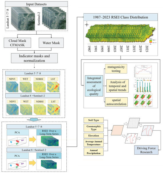
Figure 1.
Technical flow chart of the study.
2. Materials and Methods
2.1. Overview of the Study Area
Fujian Province is located in southeastern China (Figure 2), between latitudes 23°33′ and 28°19′ N and longitudes 115°50′ and 120°40′ E. It borders the East China Sea to the east, Guangdong Province to the south, Jiangxi Province to the west, and Zhejiang Province to the north. Covering an area of approximately 121,400 square kilometers, Fujian features a subtropical monsoon climate characterized by warm and humid conditions. The average annual temperature ranges from 17 °C to 21 °C. Annual precipitation is abundant, ranging from 1400 mm to 2000 mm. The terrain of Fujian is predominantly mountainous and hilly, accounting for over 80% of its total area. Major mountain ranges include the Wuyi, Daiyun, and Jiufeng ranges. The average elevation is about 500 m, with the highest peak being Mount Huanggang, at 2158 m. Fujian is crisscrossed by numerous rivers, the largest of which is the Min River, stretching approximately 577 km. With an average flow rate of about 2500 cubic meters per second, it flows through Fuzhou before emptying into the East China Sea. In addition, there is the Jiulong River, which has a total length of about 258 km and an average flow rate of about 500 cubic meters per second, as well as many smaller rivers and streams, such as the Meijiang River, Jinxi River, and Mulan River. Fujian boasts a high forest coverage rate of 66.8%, the highest in China, with major tree species including pine, fir, camphor, and bamboo. The province is rich in natural resources and is known for its fertile land, suitable for cultivating various crops such as rice, sweet potatoes, tea, and fruits. This extensive forest cover not only reflects Fujian’s lush vegetation, but also highlights its ecological importance. The abundant forests play a vital role in maintaining the ecological balance, and are crucial for conservation efforts in the region (Figure 2).
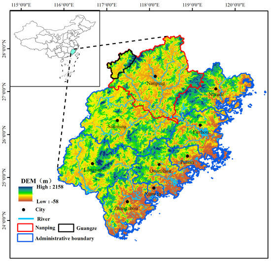
Figure 2.
Location of the study area.
2.2. Data Acquisition and Preprocessing
In this study, a strategic selection of remote sensing imagery was made to effectively monitor and analyze the ecological environmental quality of Fujian Province. We utilized Landsat 5/7/8 Level-2 and Sentinel-2 Level-2 Surface Reflectance Images, all sourced from the GEE platform. To simplify our data processing workflow, we eliminated steps such as atmospheric correction, as these are inherently handled in the Level-2 data products provided by GEE. For temporal coverage, we selected 120 to 147 Landsat TM/OLI images per year, from April to September, for the period 1987 to 2023, and 30 to 50 Sentinel-2 MSI images per year from 2019 to 2023. Detecting and removing clouds and cloud shadows is a critical step in ensuring the data quality. This process requires the use of cloud masking algorithms specifically designed for Landsat and Sentinel images. After cloud removal, median synthesis was used to generate cloud-free images for each year. While the median synthesis method effectively reduces the impact of major outliers (such as clouds and shadows), it may still include subtle outliers that deviate slightly from normal values, such as temporary changes in vegetation. These outliers may not be fully excluded by the median, which could result in images that do not fully capture short-term but ecologically significant events occurring within the season. Therefore, this study utilized a large volume of image data to ensure that a sufficient number of images were used each year, minimizing the effects of clouds and temporal inconsistencies. Additionally, this study used the Modified Normalized Difference Water Index (MNDWI) to mask water body information, ensuring that the WET accurately represents the true surface moisture conditions and avoids being affected by water. Since Sentinel lacks temperature sensors, this experiment combines Landsat and Sentinel datasets, combining Landsat’s LST dataset with Sentinel’s NDVI, WET, and NDBSI datasets, to construct RSEI.
Topographic and geomorphological data were accessed at the following link: https://www.resdc.cn/ (accessed on 4 June 2024), and average temperature data and average precipitation data are from the National Tibetan Plateau Science Data Center platform at https://data.tpdc.ac.cn/ (accessed on 26 July 2024).
2.3. Theory and Method
2.3.1. Construction of the Remote Sensing Ecological Index (RSEI)
The RSEI is a comprehensive indicator used to assess ecological environment quality. It combines factors closely related to the ecological environment, such as greenness, wetness, heat, and dryness, which correspond to the NDVI, WET, LST, and NDBSI [41], thereby reflecting the quality of the ecological environment within a region. Given the disparate dimensions and value ranges of these indices, standardization is essential to mitigate the influence of scale differences on weighting calculations [42]. Additionally, before performing Principal Component Analysis (PCA), this study used Modified Normalized Difference Water Index (MNDWI) [43] to mask water bodies, in order to reduce their influence on the principal component loadings [44]. The NDVI serves as the greenness index, indicative of vegetation health. The WET, derived from the Landsat and Sentinel Tasseled Cap Transformation [45,46], represents the moisture content in water bodies, soil, and vegetation. This transformation has found extensive application in ecological environmental monitoring. The NDBSI, comprising the Bare Soil Index (SI) and Built-Up Index (IBI), reflects the degree of aridity in the landscape [47]. LST, representing the warmth index, is retrieved using atmospheric correction methods [48]. PCA is employed to compute the first principal component (PC1) from these standardized indices. To align PC1 with the concept that higher values indicate superior ecological environmental quality, we subtract PC1 from 1, thus deriving the RSEI. This index ranges between 0 and 1, with values closer to 1 denoting better ecological environmental quality. The formulation of RSEI is designed to provide a comprehensive, quantifiable measure of ecological health, integrating diverse environmental parameters into a single, interpretable metric. The specific calculation formula is shown in Table 1.

Table 1.
Formulas and references.
2.3.2. Mann–Kendall Mutation Test
To capture the time points at which significant changes in the average RSEI occur, this study introduced a non-parametric statistical method—the Mann–Kendall Mutation Test, which is not affected by a few outliers [49,50]. The mean values were used to determine the environmental change trends in Fujian Province. For the time series RSEIi, an ordered sequence ri was constructed, representing the cumulative number of samples where RSEIi > RSEIj (1 ≤ j ≤ i). The UBk and UFk curves were obtained, and mutation points were identified through changes in these curves.
2.3.3. Spatial–Temporal Changes Analysis
To understand the change trends of RSEI over a long-term series, this study introduces Sen + Mann–Kendall trend analysis to identify the temporal changes in ecological environmental quality. This approach aims to reveal differences in environmental quality among different ecosystem types. Sen’s slope estimator can better reduce outlier interference by calculating the median of the time series [51], but it cannot judge the significance of the time-series trend by itself. Sen’s slope estimator β is defined as
where median () represents the median, if βRSEI > 0, it indicates an increasing trend in RSEI, and if βRSEI < 0, it indicates a decreasing trend.
The Mann–Kendall test is a non-parametric trend test method that is not affected by missing values and outliers [52]. Introducing the M-K test allows for the significance testing of Sen’s slope estimator [38]. The null hypothesis H0 assumes that the time series (RSEI1,…, RSEIn) consists of n independent and identically distributed samples, showing no specific upward or downward trend. The alternative hypothesis H1 is a two-tailed test, stating that for all k, j ≤ n, and k ≠ j, the distributions of RSEIk and RSEIj are different. The test statistic is denoted as S:
This study employs a two-tailed trend test, conducting significance tests at a significance level α = 0.05. The critical value Z(1 − α/2) = ±1.96. When |Z| exceeds 1.65, 1.96, and 2.58, it indicates that the trend has passed significance tests with confidence values of 90%, 95%, and 99%, respectively.
2.3.4. Spatial Autocorrelation Analysis
Spatial autocorrelation analysis is a statistical method used to measure the distribution characteristics and relationships of spatial data [53]. It is an important indicator for examining whether a specific element, such as ecological environmental quality, is correlated with the ecological environmental quality of its neighboring spatial areas. It can be used to determine whether there is a correlation between the spatial distribution of RSEI and the ecological environmental quality in adjacent regions and to quantify the strength of this correlation. Global Moran’s I and Local Moran’s I are the main indicators for calculating spatial autocorrelation, used to analyze both global and local spatial clustering of RSEI.
Global Moran’s I is a statistical measure used in global spatial-autocorrelation analysis, primarily employed to comprehensively assess spatial data across the entire study area. It reflects whether spatial data tend to exhibit clustering or dispersion, and provides insights into the strength and significance of these trends. Its values range from [−1, 1]. When its value is greater than 0, it indicates a positive spatial correlation, meaning adjacent features exhibit a “high–high, low–low” clustering trend. When its value is less than 0, it indicates a negative spatial correlation, suggesting adjacent features exhibit a “high–low or low–high” distribution trend. When its value is close to 0, it indicates spatial randomness, showing no apparent correlation.
where xi and xj are the RSEI values of each grid i and j, is the average RSEI value, wij is the spatial weight between elements i and j, and n is the number of elements.
Local Moran’s I is primarily used for analyzing spatial data in different regions or units within a study area, reflecting the degree of spatial variation and significance between each region or unit and its surrounding areas. In comparison to Global Moran’s I, Local Moran’s I focuses on detecting local spatial patterns. It can be utilized to identify different types of spatial clustering or dispersion phenomena, such as high-value clusters, low-value clusters, high–low outliers, and low–high outliers, within the study area. This local analysis helps in identifying hotspots, cold spots, or spatial-outlier points significantly different from their surrounding areas in geographic distribution. Through Local Moran’s I, one can explore the local variations in spatial data in finer detail, leading to more targeted insights.
the variables xi, xj, , and wij involved in this equation share the same parameters as Global Moran’s I.
2.3.5. Geodetector
The Geodetector is a statistical method used to detect the driving factors behind geographical phenomena and their spatial heterogeneity [54]. It is primarily based on the theory of spatial variation, revealing the reasons for the occurrence of and change in a geographical phenomenon by comparing the characteristic differences of different spatial units. This method does not rely on any linear assumptions, and can handle both numerical and categorical data. It can detect relationships between numerical data and analyze spatial heterogeneity in categorical data, offering a new perspective for understanding spatial data [55]. The Geodetector includes four main detectors: (1) Factor detector: evaluates the explanatory power of a single factor on a geographical phenomenon, i.e., the extent of the factor’s impact on the spatial distribution of the phenomenon, usually represented by q. (2) Interaction detector: evaluates the interaction between multiple factors, identifying the combination of factors that have the greatest impact on the geographical phenomenon under specific environmental conditions. (3) Risk-area detector analyzes the spatial distribution differences of risks in different areas. (4) Ecological detector: explores the impact of the interaction between two factors on a geographical phenomenon, determining whether there is a synergistic or inhibitory effect between factors, usually represented by F. These detectors assess how independent variables affect the spatial distribution of the dependent variable, detecting the explanatory power of different factors and their interaction effects on the target variable. This study selects the RSEI from 1987–2023 as the dependent variable, soil type (A1), geomorphic type (A2), elevation (A3), average annual temperature (A4), and annual precipitation (A5) as independent variables for analysis, as these factors directly or indirectly affect plant growth.
the range of q is 0–1, and the closer q is to 1, the stronger the explanatory power of the independent variable on the dependent variable, and the more consistent it is with the spatial distribution pattern of the geographical phenomenon. Nh and N represent the number of samples within layer h and the total number of samples, respectively. σh and σ represent the variance of Y within layer h and the total variance, respectively. SSW is the sum of variances within layers, and SST is the total variance. SSWx1 and SSWx2 represent the sum of variances for each category formed by independent variables x1 and x2, respectively. Nx1 and Nx2 represent the number of samples for independent variables x1 and x2, respectively. L represents the number of categories of independent variables. Y indicates a significant difference, and N indicates no significant difference.
3. Results
3.1. Comprehensive Ecological Environment Assessment
In this study, in addition to constructing the RSEI of Fujian Province, we also constructed the RSEI of Nanping City, as well as Guangze County, at the same time, and constructed the RSEI of the three separately from each other, so as to ensure the validity. The RSEI PCA results shown in Table 2 highlight the contribution of the first principal component (PC1) and the loadings of the components in the Landsat dataset and the combined Landsat and Sentinel dataset. The average contribution of PC1 was 84.26% in Fujian Province, 72.39% in Nanping City, 83.53% in Guangze County for the Landsat dataset, and 77.40% in Guangze County for the Landsat–Sentinel dataset. It shows that PC1 captures most of the characteristic information from the four indicators, and accurately represents the overall ecological characteristics of the study area. Examining the PC1 loadings reveals consistent trends: NDVI and WET have positive values, while LST and NDBSI have negative values. This pattern suggests that NDVI and WET positively influence the ecological environmental quality in Fujian Province, whereas LST and NDBSI have a negative impact. Notably, the NDVI value exceeded that of WET, indicating a stronger positive effect on PC1. In contrast, the NDBSI value surpassed that of LST, suggesting a more significant negative impact. The absolute value of NDVI is greater than that of NDBSI, further emphasizing its important influence on PC1. The contribution value of NDVI in Fujian Province generally remained at a high level, with occasional fluctuations. For example, it was 0.88 in 1987, rose to 0.89 in 1988, and remained high over the years, with slight declines in certain years, such as 1990 (0.72). Nanping City showed a similar trend, with the NDVI value increasing from 0.57 in 1990 to 0.79 in 2013, indicating periods of decline and recovery. The NDBSI contribution value was −0.55 in 1987 and −0.65 in 2023, suggesting that areas with lower soil and building density are associated with better ecological quality. A similar trend was observed in Nanping City, where the NDBSI contribution value fluctuated between −0.32 in 1987 and −0.38 in 2010, indicating that, over time, built-up areas and bare soil had varying degrees of negative impact on ecological quality. The LST contribution value fluctuated over time, with a significant increase in 2005 (−0.40) compared to earlier years such as 1987 (−0.11). The LST in Nanping City remained relatively stable but negative, reflecting its inverse relationship with NDVI. The values ranged from −0.16 in 1987 to −0.06 in 2021. The WET contribution value in Fujian Province showed little change over the years, from 0.33 in 1987 to 0.08 in 2010, indicating fluctuations in environmental moisture content. Nanping City also exhibited a similar trend, ranging from 0.02 in 1988 to 0.29 in 2011, reflecting the fact that changes in humidity levels may be related to variations in precipitation or water resource-management practices. NDVI is directly influenced by the health and density of vegetation, with naturally higher values in areas with greater vegetation cover. Seasonal changes, afforestation efforts, and land use changes (such as urban expansion or agricultural cultivation) are key factors controlling NDVI. As NDVI increases, LST typically decreases, due to the cooling effect of vegetation, NDBSI decreases due to reduced bare soil and built-up areas, and WET increases, as healthy vegetation retains more moisture. Urbanization often reduces vegetation cover, leading to lower NDVI values, higher LST, and increased NDBSI, due to the expansion of built-up areas and bare soil. This is clearly seen in the fluctuations of these indices in Fujian Province and Nanping City, where urbanization may have contributed to the decline in NDVI, the rise in LST and NDBSI, and the decline in WET, in certain years. Climate conditions such as temperature and precipitation also play a crucial role. Wetter and cooler conditions favor higher NDVI and WET values, and lower LST and NDBSI values, while drier and hotter conditions lead to higher LST and NDBSI values, reflecting reduced vegetation cover, lower moisture content, and increased soil exposure. Activities such as deforestation, agricultural expansion, and infrastructure development can cause changes in all four indices. In PC1, NDVI and WET dominate, indicating that vegetation and moisture play key roles in maintaining ecological quality, roles that may have been strengthened by conservation efforts in recent years. Similarly, the negative impacts of LST and NDBSI highlight the adverse effects of reduced vegetation, increased built-up areas, and decreased moisture content on ecological health.
Table 2.
Four indicator loadings and PC1 contributions.
Figure 3 illustrates the temporal analysis of the mean values of RSEI for the Landsat dataset for Fujian Province and Nanping City from 1987 to 2023 and for the Landsat dataset for Guangze County between 2019 and 2023 with the Landsat–Sentinel dataset, which highlight the long-term trend of the ecological environmental quality in the region. The ecological environment quality of Fujian Province has fluctuated over a certain period of time; e.g., the RSEI showed an upward and then a downward trend between 1987–1996 and 1996–2008. However, the overall trend is upward. The average value of RSEI rises from 0.57 in 1987 to 0.82 in 2023, an increase of 43.86%. The lowest point is 0.57 in 1987 and the highest point is 0.85 in 2019, an increase of 49.12%. However, Nanping and Fujian Province averages as a whole show a similar pattern, with the RSEI average rising from 0.57 in 1987 to 0.78 in 2023, an increase of 36.84%. The lowest point is 0.54 in 1989, and the highest point is 0.81 in 2022, with an increase of 50%. This upward trend indicates a gradual improvement in the quality of the ecological environment, which may be attributed to effective environmental governance and protection efforts. As for the RSEI values constructed from different datasets in Guangze County, from 2019 to 2023, the RSEI values always remain above 0.70, despite some fluctuations. This indicates that the quality of the ecological environment has remained at a high level in recent years. Meanwhile Sentinel-2 combined with Landsat dataset is able to evaluate the ecological environment quality of the region.
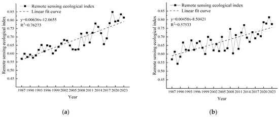
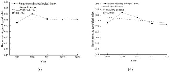
Figure 3.
The average variation of RSEI (a) Fujian LD; (b) Nanping LD; (c) Guangze LD; (d) Guangze S-L.
3.2. RSEI Mutation Analysis
Figure 4 presents the results of the Mann–Kendall mutation test, providing a detailed temporal analysis of changes in the ecological environment quality of Fujian Province. From 1985 to 1995, the UF curve fluctuated significantly but showed little overall change, indicating no substantial mutation in RSEI. The UB curve, however, had a generally downward trend, suggesting a negative change in the data, though it was not significant. Between 2000 and 2010, the UF curve gradually rose, indicating a significant positive change in the data during this period. Meanwhile, the UB curve continued to decline, reaching its lowest point in 2010, signifying a significant negative change. Post-2010, the UF curve rose markedly, especially after 2015, indicating a notable mutation in the data. Although the UB curve showed some recovery, it remained relatively low, suggesting a weakening of the negative trend during this period. Throughout the entire time series, significant changes are indicated when the UF or UB curve exceeds ±1.96, such as in 1995. The UF curve surpassed 1.96 multiple times after 2005 and 2015, highlighting significant data changes during these periods. These findings align with the average RSEI change trends, emphasizing turning points in the region’s ecological health. To better understand the temporal dynamics of ecological changes, this study focuses on specific time points for in-depth trend analysis: 1987, 1995, 2000, 2010, 2015, and 2023. This approach enables a comprehensive examination of the evolution of ecological environment quality in Fujian Province, identifying periods of deterioration and recovery.
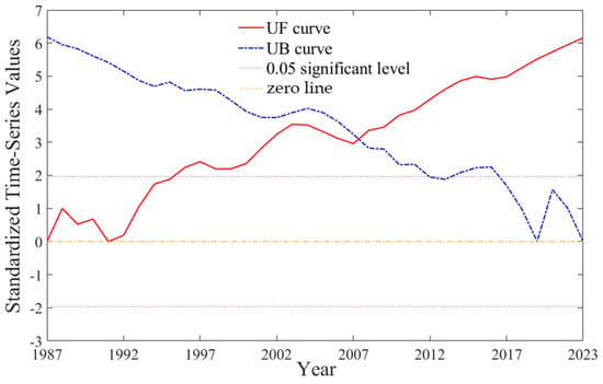
Figure 4.
Detection of RSEI Mann–Kendall mutation points.
3.3. Spatial–Temporal Characteristics of Ecological Environmental Quality
To gain a deeper understanding of the spatial–temporal dynamics in Fujian Province’s ecological environment quality, this study categorizes RSEI values into distinct intervals of 0.2. These categories are defined as Poor (0–0.2), Fair (0.2–0.4), Moderate (0.4–0.6), Good (0.6–0.8), and Excellent (0.8–1). This classification allows for a nuanced assessment of ecological quality, providing a clearer understanding of the varying degrees of ecological health across different areas of the province. The study calculates the areas and percentages corresponding to each ecological category for each defined period, visually represented in Figure 4. This figure offers a comprehensive overview of the distribution of ecological categories over time. Additionally, Figure 5 illustrates the changes in area for these categories, providing insights into the trends and shifts in ecological environment quality across different periods. This categorization and subsequent area analysis serve as critical tools for interpreting the RSEI data in a spatial–temporal context. By delineating the county into these ecological quality categories, the study effectively captures the variations and transformations in the region’s ecological landscape. Moreover, the area change analysis provides a quantifiable measure of these transformations, highlighting areas of improvement, decline, or stability in ecological quality.
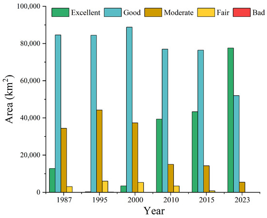
Figure 5.
Area of different levels of RSEI values.
3.3.1. Temporal Changes in Ecological Environmental Quality
This study examines the trends in ecological environment quality in Fujian Province from 1987 to 2023, using RSEI data. Understanding these trends is essential for grasping the dynamic changes in the region’s ecological environment during specific periods. As shown in Figure 5, the area rated as “Good” or “Excellent” in ecological environment quality has consistently exceeded 80%, since 2010. In 1987, 72.22% of the area was rated “Good” or above. However, in 1995 and 2000, the percentage dropped below 70%, indicating a decline in ecological environment quality. Specifically, the proportion of areas rated “Good” or above decreased from 72.22% in 1987 to 62.78% in 1995. Notably, the area rated as “Excellent” plummeted from 9.50% to just 0.19% during the same period, while the area rated as “Moderate” increased. After 2010, the ecological environment quality improved significantly, with the area classified as “Good” or better soaring to 96.06% by 2023, a substantial increase of 33.29%, compared to 1995. Throughout the period from 1987 to 2023, except for 2023, the area rated as “Good” consistently exceeded 50%, reaching 72.36% in 2023. Overall, the results indicate that the ecological environment quality in the study area first declined and then rose from, 1987 to 2023.
Figure 6 illustrates the changes in the ecological levels of Fujian Province over 37 years, as captured by the Landsat remote-sensing satellite series. The data indicate a significant overall improvement in the province’s ecological environment quality. From 1987 to 1995, there was a slight increase in ecological quality. During this period, 52.61% of the provincial area showed mild improvement, 60.76% experienced improvement, and 35.29% saw mild degradation. Between 1987 and 2000, the ecological environment remained relatively stable, with a slight reduction in areas of mild improvement. In this period, 91.79% of areas showed non-significant changes, while 53.49% experienced improvement. From 2000 to 2010, ecological health gradually improved, with the proportion of significantly improved areas exceeding those of significant degradation by 4.30%. Between 2010 and 2015, ecological quality stabilized again, with non-significant changes accounting for 86.61% of the area and 54.96% showing improvement. From 2015 to 2023, ecological quality continued to rise, with 90.24% of areas showing improvement, reflecting a significant increase in RSEI values. In summary, Figure 6 demonstrates a long-term and notable improvement in the ecological environment quality of Fujian Province.
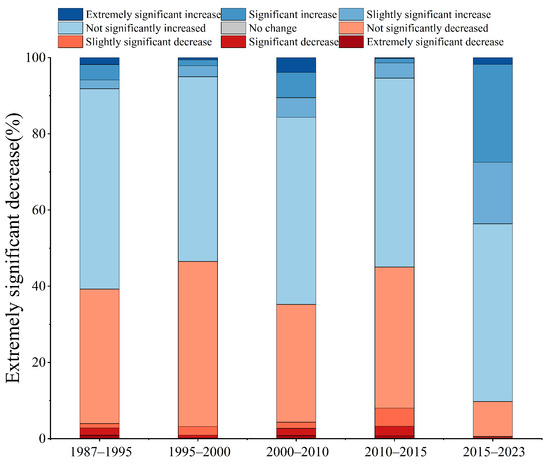
Figure 6.
Areas of different-significance changes.
Combining the results of Figure 5 and Figure 6, it can be observed that although there were more areas with increased RSEI values between 1987 and 1995, as shown in Figure 6, the area of high-grade regions actually decreased, as shown in Figure 5. This suggests that while the values increased, they may not have exceeded the 0–0.2 range that defines the grade intervals, whereas areas with decreasing values may have crossed the grading threshold, leading to an increase in the area classified as “ Moderate” in the subsequent year. This situation is most likely due to a reduction in vegetation, such as deforestation. Between 1995 and 2000, the areas with decreasing RSEI values further increased, but the area of high-grade regions also increased, indicating that during these years, the damage to the ecosystem was less than the ecosystem’s regeneration capacity, with many areas previously classified as “Good” being upgraded to “Excellent”. From 2000 to 2023, the area of high-grade regions continued to increase, while the area classified as “Moderate” gradually decreased, and the proportion of areas with significant increases in RSEI values also rose, indicating a continuous improvement in the ecological environment quality in Fujian Province over these years.
3.3.2. Spatial Changes in Ecological Environmental Quality
Figure 7 illustrates the changes in ecological and environmental quality classes in Fujian Province over time, from 1987 to 2023. The bandwidth at each time point represents the proportion of area within each quality class (Poor, Fair, Moderate, Good, and Excellent). The flow of bands between years shows the transition between quality classes. Between 1987 and 1995, the most notable change was a decline from “Excellent” to “Good”, with only a small portion of areas retaining the “Excellent” rating. Many areas previously rated as “Good” dropped to “Moderate”, indicating a noticeable decline in ecological environment quality. From 1995 to 2000, some areas shifted from “Moderate” to “Good”, and the area rated as “Excellent” also increased. However, this positive trend reversed after 2010. Gradually, areas rated as “Excellent” increased again, primarily due to the transformation of areas initially rated as “Good”. This shift marked the beginning of ecological recovery in Fujian Province. Starting from 2010, areas rated as “Good” gradually transitioned to “Excellent”, with the “Excellent” area reaching its maximum in 2023. This reinforces the trend of ecological improvement. Throughout the period from 1987 to 2023, the trend in the “Moderate” category mirrored the opposite of the “Excellent” category. These changes demonstrate that, after an early decline, Fujian Province’s ecological environment achieved significant improvement through effective governance and protection measures, reaching its optimal state in 2023.
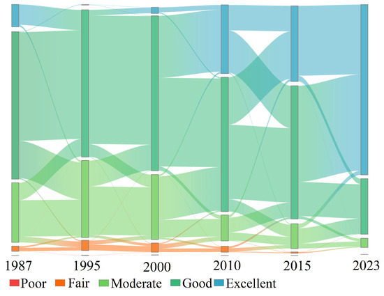
Figure 7.
Sankey diagram of ecological and environmental quality grade-transfer matrix.
3.4. Spatial Autocorrelation of RSEI
To identify the spatial pattern of RSEI distribution in Fujian Province, this study utilized Local Moran’s I statistic for spatial autocorrelation analysis. A grid framework was established across the province, consisting of 48,194 grid units. The RSEI value for each grid unit was determined by the pixel at its geometric center. Figure 8a presents the Global Moran’s I values for RSEI from 1987 to 2023 as 0.69, 0.50, 0.50, 0.54, 0.71, and 0.51. These values exceed the 1%-significance threshold, confirming the spatial autocorrelation of RSEI with 99% confidence. The positive Moran’s I values indicate an overall positive spatial correlation, with varying degrees of clustering within the regions. To visually display the local spatial distribution patterns of ecological environment quality, the Local Moran’s I statistic was used to analyze the spatial associations between geographic units, resulting in LISA cluster maps (Figure 9). These maps reveal that areas with relatively high ecological environment quality are primarily located in the mountainous regions of western Fujian Province, classified as “high–high” clusters. These areas are characterized by higher elevations, complex terrain, and minimal human disturbance. Conversely, areas with lower ecological-environment quality are predominantly found in urban areas, densely populated towns, and coastal cities, marked by low vegetation cover and intense human activities. A “high–low” buffer zone exists between the “low–low” clusters along the coast and the “high–high” clusters inland, reflecting actual conditions. From 1987 to 2023, the northeastern part of Fujian Province gradually transitioned from “low–low” clusters, indicating environmental improvement. Scattered “low–high” clusters within non-coastal regions correspond to urban areas of various counties and cities. Agricultural clusters are less pronounced, due to variability in crop phenology across different years, leading to a lack of consistent spatial patterns. Spatial autocorrelation analysis provides important insights into the distribution and clustering of ecological environment quality in Fujian Province. The findings highlight the influence of geographic features and human activities on ecological patterns, offering valuable guidance for formulating targeted environmental management and protection strategies.
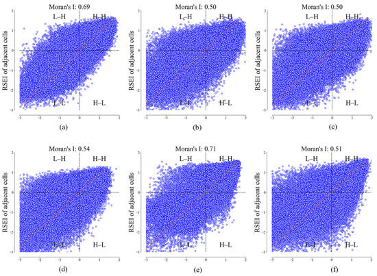
Figure 8.
Moran scatter plot of RSEI: (a–f) represent 1987, 1995, 2000, 2010, 2015, and 2023.
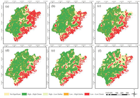
Figure 9.
LISA cluster map of the RSEI: (a–f) represent 1987, 1995, 2000, 2010, 2015, and 2023.
3.5. Analysis of Factors Affecting Ecological and Environmental Quality
3.5.1. Single-Factor Detection Analysis
In investigating the determinants of changes in ecological environment quality in Fujian Province, this study utilized the factor-detector component of Geodetector to assess the impact of various factors on RSEI. The research findings are summarized as follows (Table 3): the analysis shows that during all study periods, the p-values for the indicators were consistently 0.00, indicating their strong explanatory power for changes in RSEI. In 1987, the q-values for all factors were relatively high, suggesting that the factors significantly explained spatial variability. The q-value for soil type (A1) was the highest, indicating that it was the most influential factor that year. In 1995, among the influencing factors, landform type (A2) had the highest q-value, while precipitation (A5) had the lowest, indicating that its impact was relatively smaller, compared with that of the other factors. In 2000, landform type (A2) again showed the highest explanatory power, similar to 1995. The impacts of temperature and precipitation remained small. Landform type (A2) continued to be the most dominant influencing factor. The q-values indicate that landform and elevation factors have a greater impact than temperature and precipitation. In 2015, the influence of elevation (A3) and landform type (A2) increased significantly, with the highest q-values observed in the dataset. The influence of factors was relatively balanced, with high q-values across all aspects. In 2023, landform type (A2) remained the most influential factor, but its impact decreased compared to 2015. Precipitation (A5) had the lowest q-value and the least impact that year. Landform type (A2) consistently showed high explanatory power in most years, particularly in 2010 and 2015. Elevation (A3) became increasingly important over time, peaking in 2015. Soil type (A1) generally had a stable influence, but was not as dominant in the later years as landform type or elevation. Temperature (A4) and precipitation (A5) had lower q-values, indicating that compared to the other factors, their influence on explaining spatial variability was smaller. The results suggest that over time, landform characteristics and elevation became increasingly important in determining spatial patterns, while the influence of soil type remained significant but secondary. The diminishing impact of temperature and precipitation in later years may indicate that other environmental or anthropogenic factors have become more dominant in shaping the landscape.
Table 3.
The results of single-factor detection.
3.5.2. Multiple-Factor Detection Analysis
This study meticulously explored the synergistic effects of various factors and their significant distinctions on RSEI using the interaction-detector and ecological-detector functions of Geodetector. The analysis results are as follows (Figure 10): the results of the interaction detector indicate that the interaction of all factors exhibits characteristics of both two-factor and nonlinear enhancement. This highlights the profound impact of factor interactions on RSEI, suggesting that the combined effects of different factors largely determine the outcomes of RSEI. In 1987, the interaction between soil type (A1) and elevation (A3) was the most significant, followed by landform type (A2). The interaction between soil type and temperature (A4) and precipitation (A5) was relatively small. Significant interactions were observed between soil type, landform type, and elevation, indicating that these factors have a greater impact on geographic patterns together than they do individually. In 1995, the interaction between soil type (A1) and landform type (A2) remained significant, while the interaction with elevation (A3) was weaker. The interaction between temperature (A4) and precipitation (A5) remained low. Compared to the previous year, the interaction with temperature began to decrease slightly. In 2000, the interaction between soil type (A1) and landform type (A2) remained strong. The interaction between elevation (A3) and temperature (A4) increased, possibly indicating a closer relationship between these two factors in shaping geographic distribution this year. In 2010, the interaction between landform type (A2) and temperature (A4) and precipitation (A5) significantly strengthened. The interaction between soil type and landform type slightly weakened. In 2015, the significant interaction between elevation (A3) and temperature (A4) became more prominent than in previous years. The interaction between soil type and other factors, especially elevation and temperature, became more evident. In 2023, the interaction patterns changed again, showing a more balanced interaction between different factors. The interaction between soil type (A1) and landform type (A2) remained strong over the years, indicating a stable relationship between the two. The interaction between elevation (A3) and temperature (A4) increased over time, suggesting that the combination of temperature and elevation increasingly influences geographic patterns. The varying interactions between precipitation (A5) and other factors indicate that precipitation’s impact on geographic patterns is complex and may be influenced by the interactions of other factors. From 1987 to 2023, the study identified 47 pairs of interacting factors, with all ecological detection results marked as Y. These findings indicate significant differences in the impact of these factor combinations on RSEI, highlighting the subtle, yet important, influences of the interactions between different factors over time.
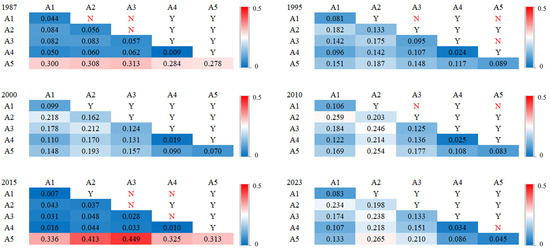
Figure 10.
Eco-detection and interactive-detection matrix.
4. Discussion
4.1. Multi-Scale RSEI Construction and Change Analysis
In constructing the RSEI, this study simultaneously built RSEIs for Fujian Province, Nanping City, and Guangze County, achieving the effect of multi-scale construction. In previous studies, researchers have tended to focus on single-scale analyses such as Xu et al. [32], Xiong et al. [35], Wen et al. [36], and Yue et al. [56]. However, constructing a multi-scale RSEI allows for a more comprehensive analysis and understanding of ecological environmental quality at different levels, as demonstrated by Huang et al. [57], who showed that multi-scale approaches can more accurately detect trends in forest changes. The principal component PC1 successfully integrated the characteristic information of the four indicators, indicating that RSEI can adapt to observations at different scales. The high contribution rate of PC1 suggests that the RSEI can robustly fit multiple surface factors and accurately reflect the quality of regional ecosystems. The positive impact of NDVI and WET on ecological health, and the negative impact of LST and NDBSI, are consistent with the findings of Liu et al. [58] in their study of northeastern China. Figure 3 shows the temporal variation of RSEI mean values in Fujian Province, Nanping City, and Guangze County, further demonstrating the effectiveness of RSEI at different scales. Although Figure 3a,b show the same overall trend, differences at different time points indicate that different characteristics are presented at different scales. Figure 3c,d, both showing monitoring results for Guangze County, display nearly identical patterns, indicating the feasibility of using Sentinel-2 data for RSEI construction. Figure 4, Figure 5, Figure 6 and Figure 7 show the temporal dynamics of RSEI in Fujian Province from 1987 to 2023. During this period, RSEI values showed an overall upward trend. From 1987 to 1995, the ecological environment quality in some areas declined. According to the literature [59] and considering climate changes in Fujian Province, the annual average temperature increased during this period, while the annual average precipitation remained stable, leading to an increase in the frequency and severity of droughts, which in turn led to a decline in ecological quality and made RSEI more volatile in some years, as noted in previous studies [60]. Between 1995 and 2000, the ecological environment began to recover, with the transition matrix showing an upward trend, indicating that the ecosystem’s self-recovery ability exceeded external disturbances. During this period, the annual average temperature continued to rise, while annual average precipitation was also higher than in previous years, thereby reducing the frequency and severity of droughts. Since 2000, the low-level areas have decreased, the high-level areas have increased, and the RSEI has remained at a high level. China’s “Grain for Green” program, launched in 2002 [61], significantly increased forest coverage in Fujian Province through reforestation efforts. Li et al. [62] highlighted an increase in carbon stocks in Fujian Province of 9.74 Tg from 1990 to 2020, mainly caused by vegetation conversion.
4.2. Spatial Autocorrelation Analysis of Ecological Environmental Quality
To ensure data integrity and promote the accurate quantitative evaluation of RSEI, this study employed resampling techniques. A total of 48,194 sampling points were extracted from each RSEI image for the years 1987, 1995, 2000, 2010, 2015, and 2023. The distribution of these sample points is crucial for understanding the spatial characteristics of ecological environment quality in Fujian Province. Moran’s I scatterplot analysis, based on the sample points, shows that most points are distributed in the first and third quadrants. This distribution pattern indicates that the ecological environmental quality in the region has a strong positive spatial correlation and clustering, which is consistent with the findings of Zhang et al. [41]. The Moran’s I value is greater than 0 each year, further confirming this conclusion and indicating that the ecological environment quality in Fujian Province is not randomly distributed, but shows significant spatial clustering. According to the distribution of mountain ranges in Fujian Province [63], high-ecological-quality mountain ranges such as the Wuyi and Daiyun Mountains show a high correlation with RSEI. Combined with the above analysis, the LISA cluster maps provide detailed visualization of these spatial patterns. From 1987 to 2023, Low–Low clusters decreased, mainly concentrated in the northeastern part of Fujian Province, reflecting an improvement in ecological quality. However, the Low–Low clustering phenomenon in the coastal areas of Fujian Province did not improve, which may be due to the impact of urbanization [7]. Coastal areas typically experience high-intensity human activities [14], such as urban expansion, industrial development, and port construction [64], leading to reduced natural vegetation and increased impervious surfaces [65], thereby lowering RSEI values. In contrast, high–high clusters are widely distributed, mainly in the inland regions of the study area. These areas have higher elevations, more complex terrain, and relatively little human interference. There is a buffer zone of high–low clustering between the coastal low–low clusters and the inland high–high clusters, as demonstrated by the findings of Hladnik et al. [66]. Scattered low–high clusters appear in non-coastal areas, corresponding to urbanized areas of counties and cities. During the urbanization process, large areas of natural land are covered by impervious materials such as concrete and asphalt [67], leading to a reduction in natural vegetation and soil moisture, significantly lowering RSEI values.
4.3. RSEI Driving Force Analysis
The study on the change in ecological environment quality in Fujian Province using Geodetector reveals important insights into dynamic changes. The analysis is divided into univariate and multifactorial examinations [68], revealing the complex interaction of natural topography and human activities in shaping the region’s ecological footprint. In the field of univariate analysis, individual statistical significance between different indicators confirms the multifaceted nature of ecological logic and the drivers of environmental quality. Among the factors influencing RSEI, topographic and geomorphic factors (terrain type and elevation) significantly outperform other factors, underscoring the foundational role of natural landscapes in ecological processes, consistent with the findings of Yang et al. [34] Multifactorial analysis further deepens this view, revealing the comprehensive influence of factor interactions on RSEI. The results show that over time, the explanatory power of landform (A2) and elevation (A3) in spatial patterns has significantly increased. This may be because these factors play a fundamental role in shaping ecosystems and vegetation distribution, especially in more complex terrains where vegetation distribution, soil formation, and hydrological processes are strongly influenced by topography. As time progresses, changes in land use (e.g., agricultural development, urban expansion) have led to the alteration of some original natural ecosystems [69], making the influence of topography and elevation more prominent. For example, in high-altitude areas, climate change may cause vegetation belts to shift upward, showing stronger spatial correlations. Soil type (A1) had stronger explanatory power for spatial patterns in the early period (e.g., 1987), possibly because of lower levels of land development at that time, making soil type a more direct influence on vegetation growth. Over time, the relative influence of soil has decreased, possibly due to increased human activities such as agricultural expansion, urbanization, and infrastructure development, which have altered the original natural landscape, leading to local changes in soil type and climate conditions, and reducing soil type’s dominance in determining vegetation distribution while the relative importance of other factors (such as topography and climate) has increased. The lower q-values for temperature (A4) and precipitation (A5) indicate their weaker explanatory power for spatial patterns. This could be related to several factors: first, climate change may have altered the original temperature and precipitation patterns, especially in temperate and subtropical regions, weakening the explanatory power of climate factors with respect to vegetation distribution [13]. Second, human interventions such as agricultural irrigation and drainage system improvements may have reduced the direct impact of precipitation on crops and vegetation, making other factors (such as topography) more important [70]. Third, during relatively long periods of climate stability, vegetation and ecosystems may have adapted to local climate conditions, making these factors less significant in the short term (e.g., interannual variability) [71]. The role of topography and elevation may become more prominent under human intervention, as certain specific topographic or elevational conditions are better suited for particular land-use types (e.g., terraced agriculture, tourism development). In summary, the observed changes are the result of the combined effects of natural environmental changes (e.g., climate change, vegetation dynamics) and intensified human activities (e.g., urbanization, agricultural development). Topography and elevation are gradually becoming dominant factors, while the influence of climate factors is gradually weakening, and the impact of soil type remains relatively stable but slightly diminished. It is worth noting that there is a certain correlation between elevation and annual average temperature and precipitation, which may affect the results of interaction detection. However, within the same elevation zone, due to the urban-heat-island effect, as shown by the study of Hua et al. [72], urban surfaces such as concrete and asphalt absorb and retain more heat than natural vegetation, leading to higher temperatures in urban areas compared to vegetation-covered areas at similar elevations. Therefore, while elevation broadly affects temperature, the heat-island effect causes local temperature increases in urban areas at lower elevations compared to vegetation-covered areas at similar elevations. These changes reflect the dynamic relationships among factors within complex environmental systems and the profound impact of human activities on the natural environment. Over the 37-year analysis period, significant changes in factor interactions were observed, highlighting the continuous evolution of these ecological parameters. As shown by the study of Feng et al. [14], over time, the impact of human activities on the ecological environment gradually became more significant. In future urban planning, relevant departments may consider increasing the construction of the “green city” model [73], which would reduce pollution, protect and restore ecosystems, mitigate climate change, improve urban resilience, and promote the sustainable use of resources. This would not only improve environmental quality within cities but also bring widespread ecological benefits to surrounding areas and the global environment [74].
4.4. Limitations and Future Prospects
Long-term sequential monitoring of ecological environment quality in Fujian Province using multi-source remote sensing data on the GEE platform has many significant advantages. First, it solves efficiency challenges common to traditional remote sensing methods, such as data downloading and image preprocessing. The GEE platform can rapidly process a large number of remote sensing images in batches, greatly simplifying the monitoring process [75]. However, there are some limitations to this study. A major limitation is the reliance on remote sensing data, which itself has limitations in terms of image resolution and quality. Although the data obtained in this study have been corrected for atmospheric conditions, urban areas typically have high population density and frequent industrial activities, which produce a large amount of exhaust gas and dust, leading to more severe air pollution. As demonstrated by Nazeer et al. [76], atmospheric correction is crucial for the quality of remote sensing images. Additionally, this study found that the fluctuations in RSEI values in mountainous areas are primarily due to the impact of terrain on different slopes, and the calculation of RSEI values is further affected by terrain effects. As shown in the study by Nie et al. [77], after terrain correction, the terrain effects are significantly reduced, thereby enhancing the utility of the images for ecological monitoring. Moreover, RSEI may not be sensitive to certain environmental changes, such as subtle changes in biodiversity and soil health, and may not fully capture detailed information about ecological changes. As a coastal province, Fujian frequently suffers from natural disasters such as typhoons and floods, causing significant short-term ecological damage. For example, Ye et al. [78] analyzed the risk of typhoon-disaster factors in different landing paths in Fujian Province. RSEI may not be able to accurately distinguish the effects of these disasters from long-term ecological trends. Future research could explore and apply more advanced image-fusion methods, such as deep learning super-resolution techniques, and combine data of different resolutions for multi-scale analysis. This would leverage the detailed information provided by high-resolution data and the temporal and spatial coverage of low-resolution data to enable a more comprehensive assessment of ecological quality. At the same time, topographic correction can be considered in mountainous areas to eliminate the impact of terrain on remote sensing images. Additionally, in the multiple-factor detection using Geodetector, although the heat-island effect may cause local temperature increases in low-altitude urban areas, balancing the detection results, future studies could consider setting different altitude gradients to conduct detection studies within the same gradient, thereby avoiding the influence of altitude. Furthermore, ecosystems are inherently complex and multifaceted. Ideally, a comprehensive assessment of ecological quality should consider more variables, beyond remote sensing data. Factors such as socioeconomic factors (carbon density, population dynamics, etc.) and climate factors are integral to ecosystems and can provide valuable insights into ecological health and sustainability [79]. Incorporating these variables into assessments can improve the depth and accuracy of ecological evaluations.
5. Conclusions
To systematically assess the long-term changes in ecological quality in Fujian Province, this study utilized the Google Earth Engine (GEE) platform to integrate Landsat and Sentinel data, constructing a multi-scale Remote Sensing Ecological Index (RSEI). The study employed Mann–Kendall mutation testing, Sen + Mann–Kendall trend analysis, Moran’s I statistics, and Geodetector, to conduct an in-depth analysis of the spatiotemporal dynamics and driving factors of ecological quality in Fujian Province. The results of the study indicate the following:
- (1)
- The integration of Landsat and Sentinel data significantly enhanced the accuracy of RSEI construction, with an average contribution rate of 84.26% for Landsat data and 77.40% for the combined Sentinel–Landsat dataset.
- (2)
- Multi-scale analysis revealed an overall upward trend in ecological quality across Fujian Province, which was evident at the provincial, municipal, and county levels, further validating the effectiveness of the multi-scale approach, particularly in areas with complex terrain.
- (3)
- Spatiotemporal analysis revealed that from 1987 to 2023, most areas in Fujian Province experienced improvements in ecological quality, while some areas underwent an initial decline followed by recovery.
- (4)
- Moran’s I analysis demonstrated significant spatial clustering of ecological quality in Fujian Province, with high-quality ecological areas concentrated in the high-altitude regions of the western part of the province, while lower-quality areas were primarily distributed in densely populated coastal cities.
- (5)
- Geodetector analysis indicated that the interaction between topographic features and natural factors played a critical role in shaping the spatial distribution of RSEI, with these interactions becoming increasingly important in areas with complex terrain, over time.
Through the integration of multi-source remote sensing data and the construction of multi-scale RSEI, this study not only significantly improved the precision and depth of ecological quality assessment, but also provided robust technical support and scientific basis for long-term ecological monitoring and environmental management in Fujian Province and similar regions. Future research will explore and apply more advanced image-fusion methods to fully utilize the detailed information provided by high-resolution data and the spatiotemporal coverage offered by low-resolution data for a comprehensive assessment of ecological quality in Fujian Province and similar areas.
Author Contributions
W.K. and W.C. contributed equally to this paper. Conceptualization, M.X., X.N. and D.M.; data curation, W.K., W.C., X.N. and D.M.; funding acquisition, X.N.; investigation, M.X., Y.L. and T.W.; methodology, W.K., W.C., M.X., Y.L. and D.M.; resources, T.W., X.N. and D.M.; software, W.K., W.C., Y.L. and X.N.; supervision, X.N.; validation, W.K., W.C., Y.L. and T.W.; visualization, W.K. and W.C.; writing—original draft, W.K. and W.C.; writing—review and editing, M.X. All authors have read and agreed to the published version of the manuscript.
Funding
This research was supported by grants from the Comprehensive Survey on Ecological Restoration in Key Areas of Wuyi Mountain of China (Number: DD20230479); the Survey of Surface Substrate in Typical Red Soil Areas of Nanping City of China (Number: DD20220865); the Obser-vation, Monitoring and Evaluation of Natural Resources and Ground Substrate in the Southeastern Hilly Region of China (Number: DD20230515); the Science and Technology Innovation Fund of Command Center of Integrated Natural Resources Survey Center (Number: KC20220013); the Remote Sensing Monitoring Technology and Dynamic Evaluation Method for Forest Ecological Quality in the Wuyishan Project of China (Number: CZDWT-2023-13).
Data Availability Statement
The original contributions presented in the study are included in the Article; further inquiries can be directed to the corresponding author.
Conflicts of Interest
The authors declare no conflicts of interest.
References
- Ying, X.; Zeng, G.-M.; Chen, G.-Q.; Tang, L.; Wang, K.-L.; Huang, D.-Y. Combining AHP with GIS in synthetic evaluation of eco-environment quality—A case study of Hunan Province, China. Ecol. Model. 2007, 209, 97–109. [Google Scholar] [CrossRef]
- Nandagiri, R. 8 Billion Lives, Infinite Possibilities: The Case for Rights and Choices; State of the World Population Report; UNFPA: New York, NY, USA, 2023; 192p, Available online: https://www.unfpa.org/sites/default/files/swop23/SWOP2023-ENGLISH-230329-web.pdf (accessed on 12 January 2024).
- Lamb, W.F.; Wiedmann, T.; Pongratz, J.; Andrew, R.; Crippa, M.; Olivier, J.G.J.; Wiedenhofer, D.; Mattioli, G.; Khourdajie, A.A.; House, J.; et al. A review of trends and drivers of greenhouse gas emissions by sector from 1990 to 2018. Environ. Res. Lett. 2021, 16, 073005. [Google Scholar] [CrossRef]
- Palo, M. Population and deforestation. In The Causes of Tropical Deforestation; Routledge: London, UK, 2023; pp. 42–56. [Google Scholar]
- Jiao, Z.; Sun, G.; Zhang, A.; Jia, X.; Huang, H.; Yao, Y. Water Benefit-Based Ecological Index for Urban Ecological Environment Quality Assessments. IEEE J. Sel. Top. Appl. Earth Obs. Remote Sens. 2021, 14, 7557–7569. [Google Scholar] [CrossRef]
- Pahl-Wostl, C. Adaptive and sustainable water management: From improved conceptual foundations to transformative change. Int. J. Water Resour. Dev. 2020, 36, 397–415. [Google Scholar] [CrossRef]
- Wang, K.; Tang, Y.; Chen, Y.; Shang, L.; Ji, X.; Yao, M.; Wang, P. The Coupling and Coordinated Development from Urban Land Using Benefits and Urbanization Level: Case Study from Fujian Province (China). Int. J. Environ. Res. Public Health 2020, 17, 5647. [Google Scholar] [CrossRef]
- Miao, L.; Pan, W.; Yang, Z. Empirical Studies on the Dynamic Relationship between Port Logistics and Marine Economic Development in Fujian Province. Math. Probl. Eng. 2022, 2022, 4086633. [Google Scholar] [CrossRef]
- Kim, H.; Jeong, H.; Jeon, J.; Bae, S. The Impact of Impervious Surface on Water Quality and Its Threshold in Korea. Water 2016, 8, 111. [Google Scholar] [CrossRef]
- Cao, Y.; Wei, J. Coupling coordination and interactive effects of new urbanization efficiency and eco-efficiency-A case study of Fujian Province. PLoS ONE 2024, 19, e0292921. [Google Scholar] [CrossRef]
- Zhou, L.; Wu, X.; Xu, Z.; Fujita, H. Emergency decision making for natural disasters: An overview. Int. J. Disaster Risk Reduct. 2018, 27, 567–576. [Google Scholar] [CrossRef]
- Turner, H.C.; Galford, G.L.; Hernandez Lopez, N.; Falcón Méndez, A.; Borroto-Escuela, D.Y.; Hernández Ramos, I.; González-Díaz, P. Extent, Severity, and Temporal Patterns of Damage to Cuba’s Ecosystems following Hurricane Irma: MODIS and Sentinel-2 Hurricane Disturbance Vegetation Anomaly (HDVA). Remote Sens. 2023, 15, 2495. [Google Scholar] [CrossRef]
- Levine, M.D.; Steele, R.V. Climate change: What we know and what is to be done. WIREs Energy Environ. 2020, 10, e388. [Google Scholar] [CrossRef]
- Feng, D.; Fu, M.; Sun, Y.; Bao, W.; Zhang, M.; Zhang, Y.; Wu, J. How Large-Scale Anthropogenic Activities Influence Vegetation Cover Change in China? A Review. Forests 2021, 12, 320. [Google Scholar] [CrossRef]
- Sergeant, C.J.; Moynahan, B.J.; Johnson, W.F. Practical advice for implementing long-term ecosystem monitoring. J. Appl. Ecol. 2012, 49, 969–973. [Google Scholar] [CrossRef]
- Pettorelli, N.; Vik, J.O.; Mysterud, A.; Gaillard, J.M.; Tucker, C.J.; Stenseth, N.C. Using the satellite-derived NDVI to assess ecological responses to environmental change. Trends Ecol. Evol. 2005, 20, 503–510. [Google Scholar] [CrossRef] [PubMed]
- Guo, Z.; Wang, N.; Shen, B.; Gu, Z.; Wu, Y.; Chen, A. Recent Spatiotemporal Trends in Glacier Snowline Altitude at the End of the Melt Season in the Qilian Mountains, China. Remote Sens. 2021, 13, 4935. [Google Scholar] [CrossRef]
- Stoms, D.M.; Hargrove, W.W. Potential NDVI as a baseline for monitoring ecosystem functioning. Int. J. Remote Sens. 2010, 21, 401–407. [Google Scholar] [CrossRef]
- Baldi, G.; Nosetto, M.D.; Aragon, R.; Aversa, F.; Paruelo, J.M.; Jobbagy, E.G. Long-term Satellite NDVI Data Sets: Evaluating Their Ability to Detect Ecosystem Functional Changes in South America. Sensors 2008, 8, 5397–5425. [Google Scholar] [CrossRef]
- Fung, T.; Siu, W. Environmental quality and its changes, an analysis using NDVI. Int. J. Remote Sens. 2010, 21, 1011–1024. [Google Scholar] [CrossRef]
- Jiang, Z.; Huete, A.; Didan, K.; Miura, T. Development of a two-band enhanced vegetation index without a blue band. Remote Sens. Environ. 2008, 112, 3833–3845. [Google Scholar] [CrossRef]
- Waring, R.H.; Coops, N.C.; Fan, W.; Nightingale, J.M. MODIS enhanced vegetation index predicts tree species richness across forested ecoregions in the contiguous U.S.A. Remote Sens. Environ. 2006, 103, 218–226. [Google Scholar] [CrossRef]
- Boucher, J.; Beaudoin, A.; Hébert, C.; Guindon, L.; Bauce, É. Assessing the potential of the differenced Normalized Burn Ratio (dNBR) for estimating burn severity in eastern Canadian boreal forests. Int. J. Wildland Fire 2017, 26, 32–45. [Google Scholar] [CrossRef]
- Giddey, B.L.; Baard, J.A.; Kraaij, T. Verification of the differenced Normalised Burn Ratio (dNBR) as an index of fire severity in Afrotemperate Forest. S. Afr. J. Bot. 2022, 146, 348–353. [Google Scholar] [CrossRef]
- Sun, G.; Jiao, Z.; Zhang, A.; Li, F.; Fu, H.; Li, Z. Hyperspectral image-based vegetation index (HSVI): A new vegetation index for urban ecological research. Int. J. Appl. Earth Obs. Geoinf. 2021, 103, 102529. [Google Scholar] [CrossRef]
- Yan, Y. Research on Saihan Dam Ecological Environment Evaluation Indexes Based on Quantitative Analysis. Acad. J. Environ. Earth Sci. 2022, 4, 1–4. [Google Scholar] [CrossRef]
- Qiao, Y.; Zhao, S.; Fang, Y. Dynamic monitoring of ecological environment based on advanced information technology. In Proceedings of the 2010 International Conference on Computer Application and System Modeling, Taiyuan, China, 22–24 October 2010. [Google Scholar] [CrossRef]
- Messer, L.C.; Jagai, J.S.; Rappazzo, K.M.; Lobdell, D.T. Construction of an environmental quality index for public health research. Environ. Health 2014, 13, 39. [Google Scholar] [CrossRef]
- Sruthi Krishnan, V.; Mohammed Firoz, C. Regional urban environmental quality assessment and spatial analysis. J. Urban Manag. 2020, 9, 191–204. [Google Scholar] [CrossRef]
- Barrera-Roldán, A.; Saldívar-Valdés, A. Proposal and application of a Sustainable Development Index. Ecol. Indic. 2002, 2, 251–256. [Google Scholar] [CrossRef]
- Xu, H. A remote sensing index for assessment of regional ecological changes. China Environ. Sci. 2013, 33, 889–897. [Google Scholar]
- Xu, H.; Wang, Y.; Guan, H.; Shi, T.; Hu, X. Detecting Ecological Changes with a Remote Sensing Based Ecological Index (RSEI) Produced Time Series and Change Vector Analysis. Remote Sens. 2019, 11, 2345. [Google Scholar] [CrossRef]
- Ning, L.; Jiayao, W.; Fen, Q. The improvement of ecological environment index model RSEI. Arab. J. Geosci. 2020, 13, 403. [Google Scholar] [CrossRef]
- Yang, H.; Yu, J.; Xu, W.; Wu, Y.; Lei, X.; Ye, J.; Geng, J.; Ding, Z. Long-time series ecological environment quality monitoring and cause analysis in the Dianchi Lake Basin, China. Ecol. Indic. 2023, 148, 110084. [Google Scholar] [CrossRef]
- Xiong, Y.; Xu, W.; Lu, N.; Huang, S.; Wu, C.; Wang, L.; Dai, F.; Kou, W. Assessment of spatial–temporal changes of ecological environment quality based on RSEI and GEE: A case study in Erhai Lake Basin, Yunnan province, China. Ecol. Indic. 2021, 125, 107518. [Google Scholar] [CrossRef]
- Wen, X.; Ming, Y.; Gao, Y.; Hu, X. Dynamic Monitoring and Analysis of Ecological Quality of Pingtan Comprehensive Experimental Zone, a New Type of Sea Island City, Based on RSEI. Sustainability 2019, 12, 21. [Google Scholar] [CrossRef]
- Yuan, B.; Fu, L.; Zou, Y.; Zhang, S.; Chen, X.; Li, F.; Deng, Z.; Xie, Y. Spatiotemporal change detection of ecological quality and the associated affecting factors in Dongting Lake Basin, based on RSEI. J. Clean. Prod. 2021, 302, 126995. [Google Scholar] [CrossRef]
- Liu, X.Y.; Zhang, X.X.; He, Y.R.; Luan, H.J. Monitoring and Assessment of Ecological Change in Coastal Cities Based on Rsei. Int. Arch. Photogramm. Remote Sens. Spat. Inf. Sci. 2020, XLII-3/W10, 461–470. [Google Scholar] [CrossRef]
- Gao, P.; Kasimu, A.; Zhao, Y.; Lin, B.; Chai, J.; Ruzi, T.; Zhao, H. Evaluation of the Temporal and Spatial Changes of Ecological Quality in the Hami Oasis Based on RSEI. Sustainability 2020, 12, 7716. [Google Scholar] [CrossRef]
- Shao, Z.; Fu, H.; Li, D.; Altan, O.; Cheng, T. Remote sensing monitoring of multi-scale watersheds impermeability for urban hydrological evaluation. Remote Sens. Environ. 2019, 232, 111338. [Google Scholar] [CrossRef]
- Zhang, Y.; She, J.; Long, X.; Zhang, M. Spatio-temporal evolution and driving factors of eco-environmental quality based on RSEI in Chang-Zhu-Tan metropolitan circle, central China. Ecol. Indic. 2022, 144, 109436. [Google Scholar] [CrossRef]
- Niu, X.; Li, Y. Remote Sensing Evaluation of Ecological Environment of Anqing City Based on Remote Sensing Ecological Index. Int. Arch. Photogramm. Remote Sens. Spat. Inf. Sci. 2020, XLIII-B3-2020, 733–737. [Google Scholar] [CrossRef]
- Ali, M.I.; Dirawan, G.D.; Hasim, A.H.; Abidin, M.R. Detection of Changes in Surface Water Bodies Urban Area with NDWI and MNDWI Methods. Int. J. Adv. Sci. Eng. Inf. Technol. 2019, 9, 946–951. [Google Scholar] [CrossRef]
- Xu, H. Modification of normalised difference water index (NDWI) to enhance open water features in remotely sensed imagery. Int. J. Remote Sens. 2007, 27, 3025–3033. [Google Scholar] [CrossRef]
- Crist, E.P. A TM Tasseled Cap equivalent transformation for reflectance factor data. Remote Sens. Environ. 1985, 17, 301–306. [Google Scholar] [CrossRef]
- Nedkov, R. Orthogonal Transformation of segmented images from the Satellite Sentinel-2. Comptes Rendus L’acad’emie Bulg. Sci. 2017, 70, 687–692. [Google Scholar]
- Xu, H.; Wang, M.; Shi, T.; Guan, H.; Fang, C.; Lin, Z. Prediction of ecological effects of potential population and impervious surface increases using a remote sensing based ecological index (RSEI). Ecol. Indic. 2018, 93, 730–740. [Google Scholar] [CrossRef]
- Malakar, N.K.; Hulley, G.C.; Hook, S.J.; Laraby, K.; Cook, M.; Schott, J.R. An Operational Land Surface Temperature Product for Landsat Thermal Data: Methodology and Validation. IEEE Trans. Geosci. Remote Sens. 2018, 56, 5717–5735. [Google Scholar] [CrossRef]
- Wang, W.; Yi, Z.; Chen, D. Mann-Kendall Mutation Analysis of Temporal Variation of Apparent Stress in Qinba Mountains and Its Adjacent Areas. IOP Conf. Ser. Earth Environ. Sci. 2021, 660, 012112. [Google Scholar] [CrossRef]
- Hamed, K.H.; Ramachandra Rao, A. A modified Mann-Kendall trend test for autocorrelated data. J. Hydrol. 1998, 204, 182–196. [Google Scholar] [CrossRef]
- Sen, P.K. Estimates of the Regression Coefficient Based on Kendall’s Tau. J. Am. Stat. Assoc. 1968, 63, 1379–1389. [Google Scholar] [CrossRef]
- Kossack, C.F.; Kendall, M.G. Rank Correlation Methods. Am. Math. Mon. 1950, 57, 425. [Google Scholar] [CrossRef]
- Chen, Y. Spatial autocorrelation equation based on Moran’s index. Sci. Rep. 2023, 13, 19296. [Google Scholar] [CrossRef]
- Zhao, Y.; Liu, L.; Kang, S.; Ao, Y.; Han, L.; Ma, C. Quantitative Analysis of Factors Influencing Spatial Distribution of Soil Erosion Based on Geo-Detector Model under Diverse Geomorphological Types. Land 2021, 10, 604. [Google Scholar] [CrossRef]
- Zhu, L.; Meng, J.; Zhu, L. Applying Geodetector to disentangle the contributions of natural and anthropogenic factors to NDVI variations in the middle reaches of the Heihe River Basin. Ecol. Indic. 2020, 117, 106545. [Google Scholar] [CrossRef]
- Yue, H.; Liu, Y.; Li, Y.; Lu, Y. Eco-Environmental Quality Assessment in China’s 35 Major Cities Based On Remote Sensing Ecological Index. IEEE Access 2019, 7, 51295–51311. [Google Scholar] [CrossRef]
- Huang, C.; Zhou, Z.; Wang, D.; Dian, Y. Monitoring forest dynamics with multi-scale and time series imagery. Environ. Monit. Assess. 2016, 188, 273. [Google Scholar] [CrossRef] [PubMed]
- Liu, P.; Ren, C.; Yu, W.; Ren, H.; Xia, C. Exploring the ecological quality and its drivers based on annual remote sensing ecological index and multisource data in Northeast China. Ecol. Indic. 2023, 154, 110589. [Google Scholar] [CrossRef]
- Huang, Q.; Qiu, Y.; Chen, X.; Sun, X.; Lin, Y. Climate Change Characteristics and Future Trends of Fujian Province During 1980–2017. J. Wuyi Univ. 2020, 39, 27–32. [Google Scholar] [CrossRef]
- Wang, Y.Q.; Yang, X.L.; Ren, L.L.; Zhang, M.R. Variation trend analysis of temperature, precipitation and drought in upper Yangtze River Basin. Yangtze River 2017, 48, 48. [Google Scholar] [CrossRef]
- Li, W.; Zinda, J.A.; Zhang, Z. Does the “Returning Farmland to Forest Program” Drive Community-Level Changes in Landscape Patterns in China? Forests 2019, 10, 933. [Google Scholar] [CrossRef]
- Li, S.; Cao, Y.; Liu, J.; Wang, S.; Zhou, W. Assessing Spatiotemporal Dynamics of Land Use and Cover Change and Carbon Storage in China’s Ecological Conservation Pilot Zone: A Case Study in Fujian Province. Remote Sens. 2022, 14, 4111. [Google Scholar] [CrossRef]
- Fang, Y.-p.; Ying, B. Spatial distribution of mountainous regions and classifications of economic development in China. J. Mt. Sci. 2016, 13, 1120–1138. [Google Scholar] [CrossRef]
- Yudina, A.; Kukushkina, Y. Construction of Low-Rise Buildings in the Coastland and Water Areas. Archit. Eng. 2021, 6, 48–53. [Google Scholar] [CrossRef]
- Liao, W.; Deng, Y.; Li, M.; Sun, M.; Yang, J.; Xu, J. Extraction and Analysis of Finer Impervious Surface Classes in Urban Area. Remote Sens. 2021, 13, 459. [Google Scholar] [CrossRef]
- Hladnik, D.; Kobler, A.; Pirnat, J. Evaluation of Forest Edge Structure and Stability in Peri-Urban Forests. Forests 2020, 11, 338. [Google Scholar] [CrossRef]
- Todeschini, S. Hydrologic and Environmental Impacts of Imperviousness in an Industrial Catchment of Northern Italy. J. Hydrol. Eng. 2016, 21, 05016013. [Google Scholar] [CrossRef]
- Wang, J.F.; Xu, C.D. Geodetector: Principle and prospective (in Chinese). Acta Geogr. 2017, 72, 116–134. [Google Scholar] [CrossRef]
- Gavrilescu, M. Water, Soil, and Plants Interactions in a Threatened Environment. Water 2021, 13, 2746. [Google Scholar] [CrossRef]
- Han, S.; Tian, F.; Gao, L. Current status and recent trend of irrigation water use in China*. Irrig. Drain. 2020, 69, 25–35. [Google Scholar] [CrossRef]
- Thom, D.; Rammer, W.; Seidl, R. Disturbances catalyze the adaptation of forest ecosystems to changing climate conditions. Glob. Chang. Biol. 2017, 23, 269–282. [Google Scholar] [CrossRef]
- Hua, L.; Zhang, X.; Nie, Q.; Sun, F.; Tang, L. The Impacts of the Expansion of Urban Impervious Surfaces on Urban Heat Islands in a Coastal City in China. Sustainability 2020, 12, 475. [Google Scholar] [CrossRef]
- Uçar, Z.; Akay, A.E.; Bilici, E. Towards Green Smart Cities: Importance of Urban Forestry and Urban Vegetation. Int. Arch. Photogramm. Remote Sens. Spat. Inf. Sci. 2020, XLIV-4/W3-2020, 399–403. [Google Scholar] [CrossRef]
- Pan, A.; Wang, Q.; Yang, Q. Assessment on the coordinated development oriented to Green City in China. Ecol. Indic. 2020, 116, 106486. [Google Scholar] [CrossRef]
- Liao, W.; Jiang, W. Evaluation of the Spatiotemporal Variations in the Eco-environmental Quality in China Based on the Remote Sensing Ecological Index. Remote Sens. 2020, 12, 2462. [Google Scholar] [CrossRef]
- Nazeer, M.; Ilori, C.O.; Bilal, M.; Nichol, J.E.; Wu, W.; Qiu, Z.; Gayene, B.K. Evaluation of atmospheric correction methods for low to high resolutions satellite remote sensing data. Atmos. Res. 2021, 249, 105308. [Google Scholar] [CrossRef]
- Nie, X.; Hu, Z.; Zhu, Q.; Ruan, M. Research on Temporal and Spatial Resolution and the Driving Forces of Ecological Environment Quality in Coal Mining Areas Considering Topographic Correction. Remote Sens. 2021, 13, 2815. [Google Scholar] [CrossRef]
- Ye, J.; Lin, G.; Zhang, M.; Gao, L. Hazard analysis of typhoon disaster-causing factors based on different landing paths: A case study of Fujian Province, China. Nat. Hazards 2019, 100, 811–828. [Google Scholar] [CrossRef]
- Sarkodie, S.A. Environmental performance, biocapacity, carbon & ecological footprint of nations: Drivers, trends and mitigation options. Sci. Total Environ. 2021, 751, 141912. [Google Scholar] [CrossRef]


Disclaimer/Publisher’s Note: The statements, opinions and data contained in all publications are solely those of the individual author(s) and contributor(s) and not of MDPI and/or the editor(s). MDPI and/or the editor(s) disclaim responsibility for any injury to people or property resulting from any ideas, methods, instructions or products referred to in the content. |
© 2024 by the authors. Licensee MDPI, Basel, Switzerland. This article is an open access article distributed under the terms and conditions of the Creative Commons Attribution (CC BY) license (https://creativecommons.org/licenses/by/4.0/).