Article

A Climate-Sensitive Mixed-Effects Individual Tree Mortality Model for Masson Pine in Hunan Province, South–Central China

1
National Forestry and Grassland Administration, Department of Planning and Finance, Beijing 100714, China
2
Forestry Science and Technology Information Research Institute of Chinese Academy of Forestry, Beijing 100091, China
3
East China Academy of Inventory and Planning of National Forestry and Grassland Administration, Hangzhou 310019, China
*
Authors to whom correspondence should be addressed.
Forests 2024, 15(9), 1543; https://doi.org/10.3390/f15091543 (registering DOI)
Submission received: 11 July 2024 / Revised: 4 August 2024 / Accepted: 24 August 2024 / Published: 1 September 2024
(This article belongs to the Section Forest Health)

Abstract

:
Accurately assessing tree mortality probability in the context of global climate changes is important for formulating scientific and reasonable forest management scenarios. In this study, we developed a climate-sensitive individual tree mortality model for Masson pine using data from the seventh (2004), eighth (2009), and ninth (2014) Chinese National Forest Inventory (CNFI) in Hunan Province, South–Central China. A generalized linear mixed-effects model with plots as random effects based on logistic regression was applied. Additionally, a hierarchical partitioning analysis was used to disentangle the relative contributions of the variables. Among the various candidate predictors, the diameter (DBH), Gini coefficient (GC), sum of basal area for all trees larger than the subject tree (BAL), mean coldest monthly temperature (MCMT), and mean summer (May–September) precipitation (MSP) contributed significantly to changes in Masson pine mortality. The relative contribution of climate variables (MCMT and MSP) was 44.78%, larger than tree size (DBH, 32.74%), competition (BAL, 16.09%), and structure variables (GC, 6.39%). The model validation results based on independent data showed that the model performed well and suggested an influencing mechanism of tree mortality, which could improve the accuracy of forest management decisions under a changing climate.

1. Introduction

Tree mortality is a key process in forest ecosystem dynamics, increasing radial growth of surrounding trees via reduced competition, promoting regeneration through the creation of gaps, returning resources to the ecosystem through the decomposition of dead trees, and creating habitats for many organisms [1,2]. Therefore, tree mortality plays an important role in shaping forest composition and structure, driving ecosystem function and influencing stand dynamics [2,3]. Usually, tree death is the result of complicated interactions among multiple factors such as competition, environmental stresses, physiology, pathology, and some random events [3,4]. Because of the complexity of the tree mortality process and the uncertainty of the time and cause of death, modelling tree mortality remains challenging [2,5].
Traditionally, tree mortality can be categorized into two types: regular mortality and irregular mortality [6,7]. Regular mortality results from suppression and competition for resources such as light, water availability, soil nutrients, and other chemical and physical agents within a stand [5]. Irregular mortality is typically caused by natural disturbances or hazards such as wildfires, hurricanes, snowstorms, insect and disease outbreaks, and some geologic hazards [8]. Generally, tree mortality models in forest growth systems have focused on regular mortality [8,9] and are divided as stand and individual tree mortality models [9,10]. Individual tree mortality models use individual trees as the basic unit and predict the survival or death probability of each tree throughout the growth period [11,12,13]. Individual tree mortality models not only show the details of stand structures and the impacts on forest management but also provide more information about the processes and factors affecting tree mortality [9,14]. Therefore, individual tree mortality models have significant advantages in predicting the probability of tree survival or death in uneven-aged mixed-species forests.
Since the response variable in tree mortality models is binary (bounded by 0 and 1), logistic or logit regression has been the most popular approach to predict the probability of survival or death of individual trees of many species [5,7,15,16]. Using logistic or logit regression to obtain unbiased estimation requires independence of observations [17,18,19]. However, since tree measurements are typically repeated and nested within plots, forestry data are typically longitudinal and nested [18,20]. Fortunately, the mixed-effects approach has been widely implemented to gain accurate estimated standard errors and statistical test results by correcting for biased estimations induced by dependence [10]. Mixed-effects approaches are extensively employed to develop forest growth and yield models such as basal area increment models [21], crown models [22,23], and height–diameter models [24,25].
The death of individual trees is influenced by multiple biotic and abiotic factors. In general, individual tree mortality models are described as a function of competition indicators, tree size or vigor, and stand features [9,26,27]. Some studies have shown that climate is also a fundamental driver of tree mortality, which shapes vegetation composition, distribution, forest structure, and function [28,29,30,31]. In addition, from the perspective of forest management, mortality risk is one of the important indices for judging whether a tree species is suitable for a specific location [5]. Climate changes significantly affect tree mortality probabilities [7,30]. Changes in the probabilities of tree mortality will not only lead to environmental variation but also have serious economic consequences. Therefore, to better inform the selection of species and practice of forest management, a climate-sensitive individual tree mortality model should be developed.
As one of the five dominant tree species in China, Masson pine (Pinus massoniana Lamb.) is extensively distributed in China, covering 10.01 million ha with a standing stock of 591 million m3. Masson pine accounts for 6.08% of the total forest area and 4.00% of the standing stock in China [32]. Masson pine-dominated forests have great ecological and socio-economical value. However, due to human or natural factors, many Masson pine forests are almost coppice forests of unreasonable stand densities, low productivities, and poor ecological functions. Their overall performance is of a poor quality, with low yields and efficiencies. It is necessary to carry out scientific and adaptive management strategies to improve the ecological and economic value of these degraded forests. This requires tree growth and yield models as a basis.
We hope that the mortality model can help forest managers to better understand the impact of climate and other variables on tree mortality and reduce economic loss to some extent by selecting more suitable tree species and formulating more scientific management strategies. In the present study, the main objectives were (1) to construct a climate-sensitive mixed-effects individual tree mortality model for Masson pine in Hunan Province, South–Central China during a 5-year time step; (2) to identify the relative contributions of the variables entering the model to tree mortality.

2. Materials and Methods
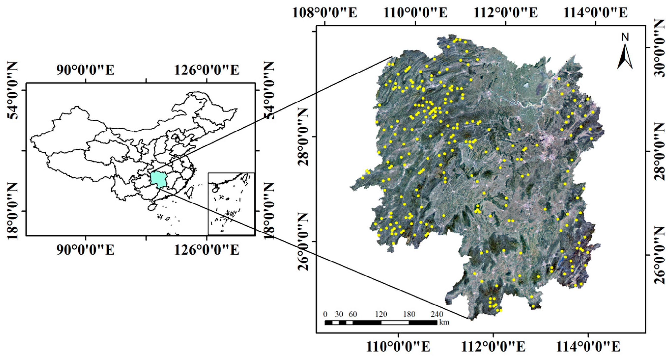
2.1. Data

The data used for this study were derived from 6615 permanent plots in the seventh (2004), eighth (2009), and ninth (2014) Chinese National Forest Inventory (CNFI) in Hunan Province, South–Central China. Each permanent plot is a 0.067 ha square, and the plots are systematically distributed on a 4 km × 8 km grid. For each plot, geographical location, elevation, slope and aspect, and individual tree information including species and diameter at breast height (DBH) for all the trees ≥ 5 cm were recorded. Additionally, each tree was identified as either dead or alive during each of the three inventory periods.
According to the “CNFI Technical Regulations”, catastrophic events causing irregular stands mortality include wildfires, forest insects and disease, climate hazards (hurricanes, snowstorms, droughts, and floods), and others. To model regular mortality, plots with catastrophic events recorded during 2004–2014 were excluded. Finally, 5921 Masson pines in 264 plots with 279 dead trees were used to study the individual tree mortality model (Figure 1). The data were randomly divided into two datasets according to the number of plots (80% of the data were used for model development and 20% for model validation). In mixed-species forests, the other important tree species were fir (Cunninghamia lanceolata), oak (Quercus spp.), sweetgum (Liquidambar formosana), and slash pine (Pinus elliottii). Additionally, several other coniferous and broad-leaved tree species occurred sporadically.
The climate variables in this study were derived from ClimateAP v2.11, which is a program used to generate climate normal, annual, seasonal, and monthly data for historical and future periods in Pacific Asia. More details can be found in ref. [33]. We obtained annual, seasonal, and monthly temperature and precipitation data by inputting the geographical coordinates (decimal degrees or degree, minute, and second) and elevation (meters) of each plot. Then, we calculated the mean temperature and precipitation per five-year period. The plots covered a range of climate conditions (Figure 2), and the mean annual temperature (MAT, °C) and precipitation (MAP, mm) showed a change during the time period of the study (Figure 3).

2.2. Variable Selection

To select appropriate predictor variables, it is necessary to understand how biological processes contribute to tree mortality rather than relying solely on fit statistics [34]. Many variables are biologically related to tree mortality and were evaluated in this study as potential predictor variables. These can be divided into five groups: (1) individual tree size variables, (2) competition variables, (3) site condition variables, (4) structural diversity variables, and (5) climate variables.

2.2.1. Individual Tree Size Variables

Individual tree size, especially DBH, is often included as an important factor affecting tree mortality [3,13,35]. Therefore, DBH was selected as a potential predictor variable. For most tree species, the mortality rate declines as tree size increases [16,36]. Goff and West confirmed that as tree size continues to increase, tree mortality rate rises again [37]. As a result, a U-shaped mortality curve may be observed [7]. To capture this trend, reciprocal transformation of DBH (DBH−1) and square of DBH (DBH2) were included as predictor variables.

2.2.2. Competition Variables

Inter-tree competition is another key variable for tree mortality modelling [1] and includes one- and two-sided competition [38]. In one-sided competition, larger trees have an advantage over smaller trees, and their growth and survival are not influenced by their smaller neighbors [39]. Competition for resources, especially for light, is the major cause of size inequality and self-thinning in dense stands [38,40]. In two-sided competition, all trees, regardless of their size, exert some competitive pressure on their neighbors and share resources equally or proportionally to their size [39,41]. Two-sided competition occurs when belowground resources such as soil nutrient and water contents are limiting [42,43]. To comprehensively quantify the competition pressure of each tree, we considered both types of competition.
One-sided competition has been captured in this study as the sum of the basal area for all trees larger than the subject tree (BAL, m2), the ratio of BAL to the DBH of the subject tree (BAL/DBH), and the ratio of the DBH of the subject tree to the quadratic mean diameter of the plot (DBH/QMD). To capture two-sided competition, quadratic mean diameter (QMD, cm), stand density (NT, stems ha−1), and basal area (BA, m2 ha−1) were selected.

2.2.3. Site Condition Variables

Site condition variables have been extensively used to predict tree mortality [6,44]. To explore the responses of tree mortality under different site conditions, we investigated elevation (EL), slope (SL), and aspect (ASP). SL and ASP were associated via Stage’s transformation, i.e., SLCos = tan (SL) × cos (ASP), ASPLn = cos (ASP) × ln (EL) [45]. Since the ages of each tree are not available, the site index, an important factor for tree mortality, was excluded.

2.2.4. Structural Diversity Variables

Forest structural diversity has a significant influence on tree mortality [46,47]. For instance, Lei found that tree mortality increased with higher tree size diversity [48]. Structural diversity is generally subdivided into three types: tree species diversity, tree size diversity, and tree position diversity [49,50]. Because of the limited availability of tree coordinate data in our study, only the diversity of tree species and size variables were included.
To determine the tree species diversity, the Shannon–Wiener index (SHI), Pielou index (PI), and Simpson’s index (SII) were used. To determine the tree size diversity, the Gini coefficient (GC) and standard deviation of the DBHs (SDDBH) were used. The equations are as follows:
SHI = i = 1 n p i × l n p i
where pi represents the proportion of basal area in the ith species.
PI = S H I ln S
In Equation (2), SHI represents the Shannon–Wiener index, and S represents the total number of species in a plot across all plots in a dataset.
SII = 1 i = 1 n p i 2
In Equation (3), pi represents the proportion of basal area in the ith species, and n represents the number of species observed.
GC = t = 1 n 2 t n 1 b a t t = 1 n b a t n 1
In Equation (4), bat represents basal area for the tree in rank t (m2 ha−1), and t represents the rank of a tree in order from 1, …, n.

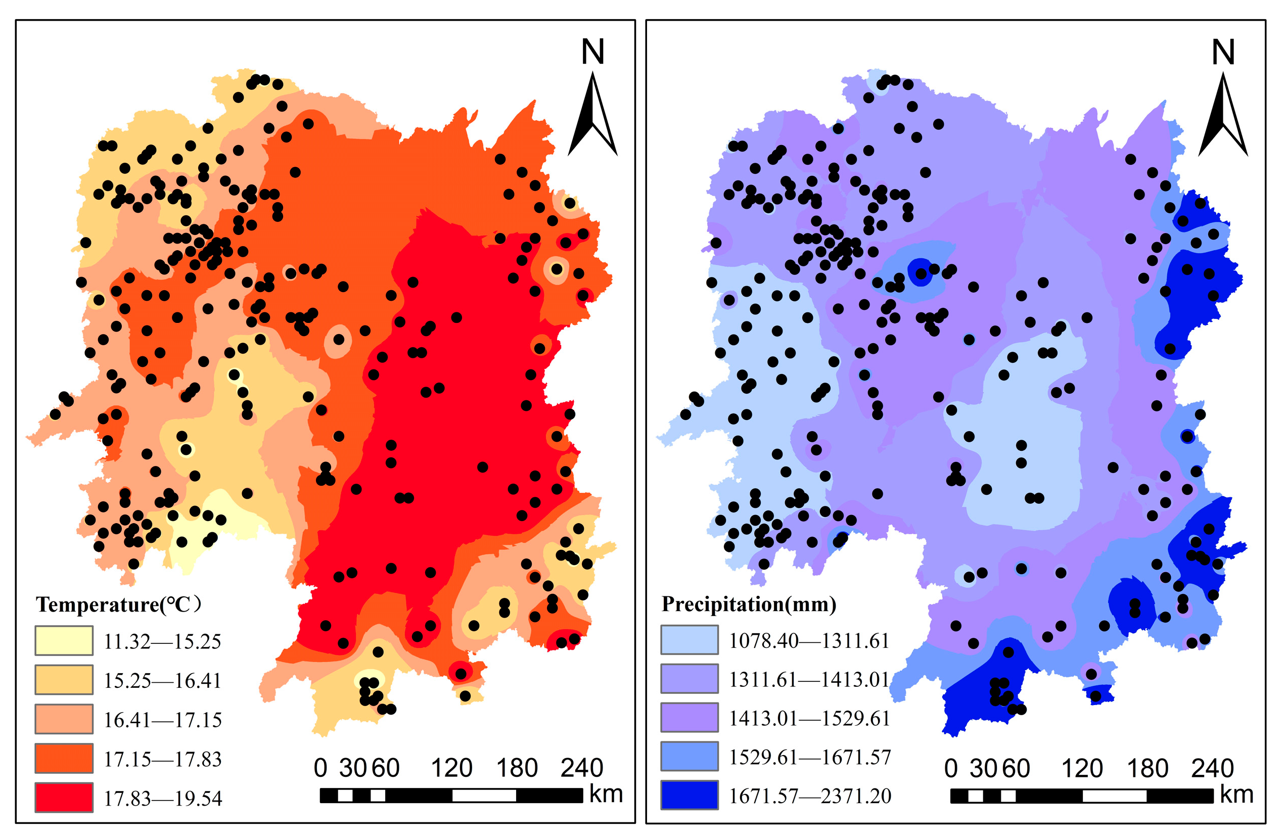
2.2.5. Climate Variables

To understand the effects of climate on tree mortality, we examined key climate variables including MAT and MAP, mean summer (May–September) precipitation (MSP, mm), mean precipitation in January (MP1, mm) and July (MP7, mm), mean warmest monthly temperature (MWMT, °C), mean coldest monthly temperature (MCMT, °C), and mean annual precipitation as snow between August in the previous year and July in the current year (PAS, mm).
The descriptive statistics of the candidate variables in this study are given in Table 1.

2.3. Generalized Linear Mixed-Effects Mortality Model Development

Because individual tree mortality is a discrete event (i.e., 0 = alive or 1 = dead), the following logistic regression model was employed to predict the mortality of Masson pine using the predictor variables described in Table 1 [2,24]:
P s = e α + β X 1 + e α + β X
The “logit” equation transformed by equation X made βX an unconstrained linear function and provided the link between βX and the predicted probability with a boundary of [0, 1] [51]. The “logit” sums as follows:
log ( P s 1 P s ) = α + β X
where Ps represents the 5-year mortality probability of each tree, X represents a matrix of explanatory variables used to develop the model, α represents an intercept, and β represents the coefficient vector to be estimated.
Among the various predictor variables tested, backward stepwise regression with Wald Chi-square tests was used. Furthermore, we calculated the variance inflation factor (VIF) to check for multicollinearity among the predictor variables. To reduce overfitting, the variables with a VIF ≥ 4 were excluded [21]. Finally, only variables with p < 0.05 based on their Wald Chi-square statistics and VIF values < 4 were retained in the model.
The plots’ random effects were added to the logistic regression model in Equation (6) to build the generalized linear mixed-effects (GLMM) mortality model. In this study, all possible combinations of the fixed-effects parameters with the random effects at plot-levels were modelled, then the best combination was selected for further analyses with the smallest Akaike information criterion (AIC), Bayesian information criterion (BIC), and −2 × Log-likelihood (−2LL). Additionally, the unstructured covariance structure was applied to account for the variance–covariance structure of plot-level random effects. The parameters were estimated with the maximum likelihood using the Lindstrom and Bates algorithm implemented using the R software (version 3.5.1) nlme function.

2.4. Model Evaluation and Validation

To evaluate model fit, the Hosmer–Lemeshow goodness-of-fit test was used to assess the difference between the predicted and observed mortality [52]. All sample trees were sorted in ascending order based on the predicted logistic probability and then split into ten groups of equal numbers [1]. The Pearson Chi-square statistic was calculated. p values < 0.05 indicated significant differences between the predicted tree mortality and the observed tree mortality at a 95% confidence level. Larger p values suggest that the predicted mortality did not differ from the observed mortality.
In addition, the receiver operating characteristic (ROC) curve and the area under the ROC curve (AUC) were calculated [52]. In the ROC curve evaluation, the true positive rate (sensitivity) was plotted against the false positive rate (1-specificity). Sensitivity is the proportion of observed positive events that were predicted to be positive events, and specificity is the proportion of observed negative events that were predicted to be negative events. The AUC values were used to measure the discriminatory power of the models [53]. If an AUC value is < 0.5, it suggests no discriminatory power; 0.7–0.8 suggests acceptable discriminatory power; and >0.8 suggests excellent discriminatory power [24,54].
For model validation, an independent dataset (i.e., 20% of the plot data) was used to predict the probability of mortality for each tree. Using the GLMM, two levels of predictions could be considered: the population average (PA) mortality, based on the fixed effects only, and the subject-specific (SS) mortality, incorporating the random effects [55]. We also calculated the AUC values to validate the mortality functions for Masson pine based on the predicted mortality probabilities.
Importantly, to disentangle the relative contributions of tree size, competition, site conditions, structural diversity, and climate variables entering the tree mortality model, a hierarchical partitioning (HP) analysis was applied using the hier.part package in R [56]. From the perspective of forest management, the independent variables that have higher relative importance values should be given higher priority in forest management planning.

2.5. Mortality Implementation Methods

Several approaches can be employed to convert the continuous probabilities generated by the mortality model into a binary result. In many previous studies, a fixed value of 0.5 was chosen as the threshold between events and non-events; however, a standard threshold of 0.5 only works if the probability of dead trees is similar to the probability of living trees. However, in fact, tree mortality is a rare event. In this study, three mortality implementation methods were compared. The first was the overall mortality rate found for the species [16], the second was the value at which the sensitivity line crosses the specificity line [52], and the third was a random number [57].
We calculated the accurate classification rates (ACRs), which were based on the confusion matrix (also called a classification table) of correct responses for the prediction of alive/dead trees, to select the optimal method.

3. Results

3.1. Generalized Linear Mixed-Effects Mortality Model

Considering the intercept and all explanatory variables as random effects, the model in which the intercept was the only random effect yielded the lowest AIC (1029), BIC (1074), and −2LL (1015, df = 7) values. Therefore, the final mortality model for Masson pine was as follows:
P S = 1 1 + E X P α + b 0 + β 1 D B H + β 2 G C + β 3 B A L + β 4 M C M T + β 5 log MSP
where b0 represents the plot-level random effect parameter. All other parameters and variables are the same as defined earlier.
All VIF values of the variables were significantly less than 4, and the parameters were significant (p < 0.05) except for GC and MCMT (GC, p = 0.342; MCMT, p = 0.633) based on their Wald Chi-square statistics (Table 2). However, removing these parameters worsened model fit; i.e., the AIC values became larger. We therefore retained the two variables in the final model. The Chi-square value of the Hosmer–Lemeshow goodness-of-fit test was 9.769 (p = 0.282), indicating that there was no evidence of significant differences between the observed and predicted mortality at the 95% confidence level (Table 2). The AUC value from the model was 0.974, indicating excellent discrimination (Figure 4).
We predicted the probability of mortality for each tree using an independent dataset to validate the model. The validated AUCs were 0.780, and 0.802 for the PA response (Equation (7) without b0) and SS response (Equation (7) with b0), respectively (Figure 5). The validated AUC values were slightly lower than the AUC from the fitting data but still showed strong model discriminatory power.

3.2. Contributions of Tree Size, Competition, Structural Diversity, and Climate Factors to Tree Mortality

According to the HP analysis, the relative contribution of MSP to tree mortality was the greatest, followed by DBH, BAL, MCMT, and the GC coefficient. The relative contribution of climate variables to mortality was 44.78%, which was larger than tree size (32.74%), competition (16.09%), and structure variables (6.39%).

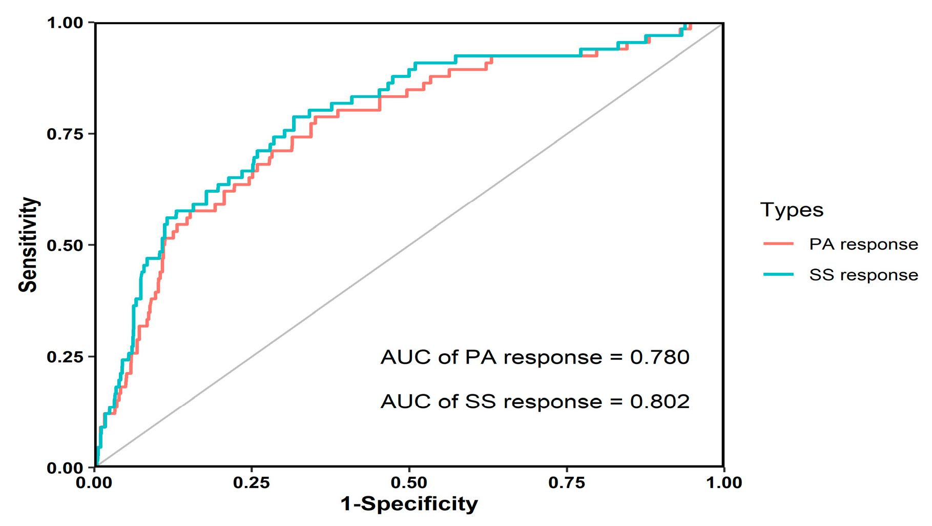
3.3. The Optimal Threshold

The model was used to predict the mortality probability of each tree after five years, and the thresholds from different mortality implementation methods were selected to assign mortality. If the predicted mortality probability exceeded the threshold, the tree was regarded as dead. After ranking the predicted mortality rates from the model, the cut-off value at which the predicted mortality reached 5% of the tree population was A = 0.25. The interception point of sensitivity and specificity was the second threshold, B = 0.06. Random numbers were fit 10 times, and the average classification rate was recorded.
The ACR was maximized at the average observed mortality rate of 0.25 (Table 3), and 4.83% of the trees were classified as dead during the 5-year time step (observed value: 4.74%). Both the interception points of sensitivity and specificity and the random number methods yielded smaller ACRs than the overall mortality rate found using the species method.

4. Discussion

In this study, a generalized linear mixed-effects model was developed to predict the mortality of Masson pine in Hunan Province, South–Central China during a 5-year time period. The model yielded an AUC of 0.802, consistent with most previous studies [2,7,9].
Based on ecological relationships and fit statistics, DBH, BAL, GC, MSP, and MCMT were included as predictors in the mortality model. The relative contribution analysis results showed that climate was the main driver (MCMT and MSP, 44.78%), followed by tree size (DBH, 33.74%), competition (BAL, 16.09%), and structural diversity (GC, 6.39%) (Table 3). Additionally, we predicted the rates of tree mortality for different values of each variable (Figure 6).

4.1. Effects of Tree Size, Competition, and Structural Diversity on Tree Mortality

Tree size (DBH) is a key factor affecting tree mortality. The negative relationship in our study suggested that tree mortality decreased as diameter increased (Figure 6). Generally, trees with larger DBHs tend to be dominant in a stand, and they exhibit higher levels of vitality and vigor [3]. Meanwhile, larger trees have advantages in competition, which leads to a higher survival rate. Some studies have shown that the correlation between DBH and tree mortality might be U-shaped [7,16]; i.e., tree mortality rates decrease with increasing DBHs but increase again above a certain limit. However, our study did not capture this U-shaped mortality trend due to the lack of larger trees in the dataset resulting from experimental stand structures with coppices and subsequent shoot or root regeneration.
The HP analysis demonstrated that inter-tree competition was also the main driver of tree mortality. The effects of competition can be interpreted as direct interference or indirect exploitation of resources [3,58]. Strong competition among trees hinders individual growth and may eventually result in death. Consistent with the results reported by Shifley [59] and Zhang [2], BAL, a one-sided competition index, was a highly significant predictor of tree mortality, and the trees were more likely to be alive when they held a higher competitive status. This may have been because for shade-intolerant species such as Masson pine, light (rather than competition for rooting space, soil water, and nutrients) is the major limiting factor for tree growth and mortality. Larger trees compete better for light and other resources since they have a well-developed rooting system. Therefore, tree mortality rate increases with the increase in BAL.
Although we included five potential independent variables describing the diversity of tree species and size (SHI, PI, SII, GC, and SDDBH) in our study, only GC remained in our final model, and the contribution was 6.39%. In our study, the tree mortality rate increased with GC. Larger GC values indicate asymmetric competition conditions in the stand, which accelerate the mortality of smaller trees. This may be attributable to the decrease in total light interception of the stand and light use efficiency to lower canopy strata and understory vegetation [60]. To better understand this effect, one could consider that tree size diversity is positively related to canopy depth and leaf area index, suggesting that stands with high tree size diversities have higher light interception efficiencies. However, this gain is inevitably accompanied by a loss of light transmittance in low canopies and understory vegetation, which in turn leads to high mortality of the smaller trees.

4.2. Effects of Climate Factors on Tree Mortality

Our results indicated that climate factors had the largest relative contribution to the mortality of Masson pine. The influence of climate is more complex than a simple monotonic relationship with precipitation or temperature. In this study, tree mortality rates decreased with an increase in MCMT but increased with an increase in MSP.
It can be seen in Figure 6 that the mortality rates of the Masson pines increased greatly when the temperature was below 0 °C. Freezing damage is regarded as a major source of stress related to reduced productivity and increased tree mortality [61,62]. Low temperatures accompanied by snow or storms lead not only to physical injuries (e.g., defoliation, tree crown/stem/branch destruction, and tree falling) but also physiological damage to trees through various processes (e.g., photoinhibition) [63,64] and cellular membrane injuries [65]. Subzero temperatures can also cause water to flow out of the cells through the imbalance of water potential between extracellular ice and intercellular water, leading to cell dehydration [66]. When freezing-induced dehydration exceeds the dehydration tolerance of the cell, the cellular membrane structure is damaged, which may result in tree death [65]. Zheng argued that even short-term freezing could cause disastrous damage to trees. Therefore, increases in minimum winter temperatures help to mitigate freezing damage and reduce tree mortality [62].
As a general rule, tree mortality probabilities were lower in warmer environments when water availability was not the limiting factor. In our study, when the temperature was higher than 0 °C, the probability of tree mortality increased with increasing MCMT (Figure 6). Warmer temperatures may increase photosynthetic activity, contributing to higher rates of carbon assimilation and faster tree growth, which in turn reduces tree mortality [2,67]. Thus, the increase in growth translates into an increase in tree vigor, which helps trees to resist pests or mechanical damage, resulting in a net reduction in mortality.
The mortality rates of the Masson pines increased sharply at high precipitation levels in this study (Figure 6), in line with results reported in earlier studies [2,68,69]. Soil with high moisture contents or water saturation can reduce the amount of oxygen in the soil, causing the death of fine roots and making trees more vulnerable to injury or death [70]. Additionally, excessive rainfall in some sites may lead to poorer soil quality due to the increase in runoff and nutrient leaching, which in turn can increase mortality rates. However, this is unlikely to be the reason for the high mortality rates in these forest stands, because large amounts of precipitation are generally the result of short-term rainfall, and most of the water becomes runoff on steep slopes. The most likely reason for the increase in mortality rates with high precipitation in summer was the strong winds that accompanied the high precipitation. As the specific causes of tree death were not recorded in our study, it is impossible to test the hypothesis that soil moisture or wind resulted in tree mortality rather than precipitation, but more detailed observations from these and other plots can be used validate or refute these propositions in the future.

4.3. Threshold Selection

In our study, the percentage of dead trees correctly classified was 65.61%, and the percentage of alive trees correctly classified was 98.20% for the model based on a threshold of 0.25. Similar results have been reported by other researchers [9,24]. Prediction and classification follow different patterns, so when selecting an optimal threshold to apply to the model, both accurate classification of dead trees and accurate prediction of mortality and survival rates must be taken into account. Because living trees generally greatly outnumber dead trees at a specific point in time in natural populations, errors that lead to an underestimate of the number of live trees may have a greater impact on predictions of tree mortality [71]. The threshold obtained using the overall mortality rate for the species predicted the highest ACR in our study. Both the interception of the sensitivity and specificity curves and the random number overestimated the mortality rate. A complete validation of mortality models must include verification that the total predicted mortality is close to the total observed mortality [72]. In our study, the random number and interception points yielded poorer results compared to the overall mortality rate. It would be meaningful to test which method of implementing individual tree mortality achieves the best results in mortality models and whether there are differences among the results reported by different researchers [9,24].

4.4. Limitations

There are some limitations of our final individual tree mortality model. Das reported that tree vigor had a significant influence on mortality, such that decreased vigor resulted in increased susceptibility to mortality agents [71]. Crown size-related variables (i.e., crown width or ratio) have been widely applied to model individual tree growth and survival [16,73]. These variables accurately reflect the effects of tree vigor, and their inclusion is preferred whenever possible, however, crown width and length were not included in our dataset. The lack of crown size-related variables may have affected our model fit. In addition, with a sufficiently long time series, an interval random effect can account for some variability resulting from catastrophic mortality caused by drought conditions, pest and disease outbreaks, windstorms, and excessive rainfall [74]. Therefore, when data from several time periods are available, time may be included as a random effect in the model to crudely estimate disturbance-related mortality.

5. Conclusions

A generalized linear mixed-effects model was developed for individual tree mortality of Masson pines in Hunan Province, South–Central China. This model described the natural mortality of Masson pine in mixed-species stands and provided information about the important variables explaining the process of individual tree mortality and the biology of their relationships with the mortality rate. The results showed that climate was the main driver (MCMT and MSP, 44.78%), followed by tree size (DBH, 33.74%), competition (BAL, 16.09%), and structural diversity (GC, 6.39%). This model may be a useful tool to simulate long-term stand dynamics based on different silviculture strategies and may contribute to the scientific management of Masson pine forests under a changing climate.

Author Contributions

All authors made significant contributions to the manuscript. Conceptualization, J.W. and Z.Z.; methodology, J.W. and K.C.; validation, N.Y. and Y.L.; database organization, Y.H. and J.W.; writing—original draft preparation, N.Y.; N.Y., J.W. and Z.Z. are the main authors who developed and revised the manuscript. All authors have read and agreed to the published version of the manuscript.

Funding

This study was not supported by funding.

Data Availability Statement

The data underlying this article cannot be shared publicly due to data security. The data will be shared by the corresponding author upon reasonable request.

Acknowledgments

The authors would like to thank their colleagues at the Academy of Forest Inventory and Planning, National Forestry, and Grassland Administration for their kind support during the data collection process.

Conflicts of Interest

The authors declare that they have no known competing financial interests or personal relationships that could have appeared to influence the work reported in this paper.

References

  1. Yang, Y.; Titus, S.J.; Huang, S. Modeling individual tree mortality for white spruce in Alberta. Ecol. Model. 2003, 163, 209–222. [Google Scholar] [CrossRef]
  2. Zhang, X.; Wang, Z.; Chhin, S.; Wang, H.; Duan, A.; Zhang, J. Relative contributions of competition, stand structure, age, and climate factors to tree mortality of chinese fir plantations: Long-term spacing trials in southern China. For. Ecol. Manag. 2020, 465, 118103. [Google Scholar] [CrossRef]
  3. Zhou, X.; Chen, Q.; Sharma, R.; Wang, Y.; He, P.; Guo, J.; Lei, Y.; Fu, L. A climate sensitive mixed-effects diameter class mortality model for prince rupprecht larch (Larix gmelinii var. Principis-rupprechtii) in northern China. For. Ecol. Manag. 2021, 491, 119091. [Google Scholar] [CrossRef]
  4. Hawkes, C. Woody plant mortality algorithms: Description, problems and progress. Ecol. Model. 2000, 126, 225–248. [Google Scholar] [CrossRef]
  5. Brandl, S.; Paul, C.; Knoke, T.; Falk, W. The influence of climate and management on survival probability for Germany’s most important tree species. For. Ecol. Manag. 2020, 458, 117652. [Google Scholar] [CrossRef]
  6. Li, Y.; Kang, X.; Zhang, Q.; Guo, W. Modelling tree mortality across diameter classes using mixed-effects zero-inflated models. J. For. Res. 2018, 31, 131–140. [Google Scholar] [CrossRef]
  7. Qiu, S.; Xu, M.; Li, R.; Zheng, Y.; Clark, D.; Cui, X.; Liu, L.; Lai, C.; Zhang, W.; Liu, B. Climatic information improves statistical individual-tree mortality models for three key species of Sichuan Province, China. Ann. For. Sci. 2015, 72, 443–455. [Google Scholar] [CrossRef]
  8. Alenius, V.; Hökkä, H.; Salminen, H.; Jutras, S. Modelling forest systems. In Proceedings of the Workshop on the Interface between Reality, Modelling and the Parameter Estimation Processes, Sesimbra, Portugal, 2–5 June 2002; pp. 225–236. [Google Scholar]
  9. Adame, P.; Río, M.; Cañellas, I. Modeling individual-tree mortality in Pyrenean oak (Quercus pyrenaica willd.) stands. Ann. For. Sci. 2010, 67, 810. [Google Scholar] [CrossRef]
  10. Timilsina, N.; Staudhammer, C. Individual tree mortality model for slash pine in Florida: A mixed modeling approach. S. J. Appl. For. 2012, 36, 211–219. [Google Scholar]
  11. Pedersen, S. Models of Individual Tree Mortality for Trembling Aspen, Lodgepole Pine, Hybrid Spruce and Subalpine Fir in Northwestern British Columbia. Ph.D. Thesis, Sveriges lantbruksuniversitet, Umeå, Sweden, 2007. [Google Scholar]
  12. Rennolls, K.; Clutter, J.; Fortson, J.; Pienaar, L.; Brister, G.; Bailey, R. Timber management: A quantitative approach. Biometrics 1983, 40, 569. [Google Scholar] [CrossRef]
  13. Yao, X.; Titus, S.; Macdonald, S. A generalized logistic model of individual tree mortality for aspen, white spruce, and lodgepole pine in Alberta mixedwood forests. Can. J. For. Res. 2001, 31, 283–291. [Google Scholar] [CrossRef]
  14. Mabvurira, D.; Miina, J. Individual-tree growth and mortality models for Eucalyptus grandis (hill) maiden plantations in Zimbabwe. For. Ecol. Manag. 2002, 161, 231–245. [Google Scholar] [CrossRef]
  15. Eid, T.; Tuhus, E. Models for individual tree mortality in Norway. For. Ecol. Manag. 2001, 154, 69–84. [Google Scholar] [CrossRef]
  16. Monserud, R.; Sterba, H. Modeling individual tree mortality for Austrian forest species. For. Ecol. Manag. 1999, 113, 109–123. [Google Scholar] [CrossRef]
  17. Allison, P. Logistic Regression Using the SAS System: Theory and Application; SAS Publishing: New York, NY, USA, 1999. [Google Scholar]
  18. Grégoire, T.; Schabenberger, O.; Barrett, J. Linear modelling of irregularly spaced, unbalanced, longitudinal data from permanent-plot measurements. Can. J. For. Res. 2011, 25, 137–156. [Google Scholar] [CrossRef]
  19. Ma, Z.; Peng, C.; Li, W.; Zhu, Q.; Wang, W.; Song, X.; Liu, J. Modeling individual tree mortality rates using marginal and random effects rgression models. Nat. Resour. Model. 2013, 26, 131–153. [Google Scholar] [CrossRef]
  20. Groom, J.; Hann, D.; Temesgen, H. Evaluation of mixed-effects models for predicting douglas-fir mortality. For. Ecol. Manag. 2012, 276, 139–145. [Google Scholar] [CrossRef]
  21. Wang, W.; Bai, Y.; Jiang, C.; Yang, H.; Meng, J. Development of a linear mixed-effects individual-tree basal area increment model for masson pine in Hunan Province, south-central China. J. Sustain. For. 2020, 39, 526–541. [Google Scholar] [CrossRef]
  22. Fu, L.; Sharma, R.; Hao, K.; Tang, S. A generalized interregional nonlinear mixed-effects crown width model for prince rupprecht larch in northern China. For. Ecol. Manag. 2017, 389, 364–373. [Google Scholar] [CrossRef]
  23. Xu, H.; Sun, Y.; Wang, X.; Wang, J.; Fu, Y. Linear mixed-effects models to describe individual tree crown width for China-fir in Fujian province, southeast China. PLoS ONE 2015, 10, e0122257. [Google Scholar]
  24. Crecente-Campo, F.; Tome, M.; Soares, P.; Dieguez-Aranda, U. A generalized nonlinear mixed-effects height-diameter model for Eucalyptus globulus L. In northwestern Spain. For. Ecol. Manag. 2010, 259, 943–952. [Google Scholar] [CrossRef]
  25. Sharma, M.; Parton, J. Height–diameter equations for boreal tree species in Ontario using a mixed-effects modeling approach. For. Ecol. Manag. 2007, 249, 187–198. [Google Scholar] [CrossRef]
  26. Hamilton, D. A logistic model of mortality in thinned and unthinned mixed conifer stands of northern Idaho. For. Sci. 1986, 32, 989–1000. [Google Scholar] [CrossRef]
  27. Wyckoff, P.; Clark, J. Predicting tree mortality from diameter growth: A comparison of maximum likelihood and Bayesian approaches. Can. J. For. Res. 2000, 30, 156–167. [Google Scholar] [CrossRef]
  28. Allen, C.; Macalady, A.; Chenchouni, H.; Bachelet, D.; Mcdowell, N.; Vennetier, M.; Kitzberger, T.; Rigling, A.; Breshears, D.; Hogg, E.; et al. A global overview of drought and heat-induced tree mortality reveals emerging climate change risks for forests. For. Ecol. Manag. 2010, 259, 660–684. [Google Scholar] [CrossRef]
  29. Mantgem, P.; Stephenson, N.; Byrne, J.; Daniels, L.; Franklin, J.; Fule, P.; Harmon, M.; Larson, A.; Smith, J.; Taylor, A.; et al. Widespread increase of tree mortality rates in the western united states. Science 2009, 323, 521–524. [Google Scholar] [CrossRef]
  30. Neumann, M.; Mues, V.; Moreno, A.; Hasenauer, H.; Seidl, R. Climate variability drives recent tree mortality in Europe. Glob. Chang. Biol. 2017, 23, 4788–4797. [Google Scholar] [CrossRef] [PubMed]
  31. Peng, C.; Ma, Z.; Lei, X.; Zhu, Q.; Chen, H.; Wang, W.; Liu, S.; Li, W.; Fang, X.; Zhou, X. A drought-induced pervasive increase in tree mortality across Canada’s boreal forests. Nat. Clim. Chang. 2011, 1, 467–471. [Google Scholar] [CrossRef]
  32. National Forestry and Grassland Administration. Report of Forest Resources in China (2014–2018); China Forestry Publishing House: Beijing, China, 2019; pp. 1–2.
  33. Wang, T.; Wang, G.; Innes, J.; Seely, B.; Chen, B. Climateap: An application for dynamic local downscaling of historical and future climate data in Asia pacific. Front. Agric. Sci. Eng. 2017, 4, 448–458. [Google Scholar] [CrossRef]
  34. Hamilton, D. Extending the range of applicability of an individual tree mortality model. Can. J. For. Res. 1990, 20, 1212–1218. [Google Scholar] [CrossRef]
  35. Jutras, S.; Hokka, H.; Alenius, V.; Salminen, H. Modeling mortality of individual trees in drained peatland sites in Finland. Silva Fenn. 2003, 37, 235–251. [Google Scholar] [CrossRef]
  36. Silvertown, J. Introduction to plant population ecology. Vegetatio 1984, 56, 86. [Google Scholar]
  37. Goff, F.; West, D. Canopy-understory interaction effects on forest population structure. For. Sci. 1975, 21, 98–108. [Google Scholar]
  38. Weiner, J. Asymmetric competition in plant populations. Trends Ecol. Evol. 1990, 5, 360–364. [Google Scholar] [CrossRef] [PubMed]
  39. Cannell, M.; Rothery, P.; David, F. Competition within stands of Picea sitchensis and Pinus contorta. Ann. Bot. 1984, 53, 349–362. [Google Scholar] [CrossRef]
  40. Weiner, S. Mechanisms determining the degree of size asymmetry in competition among plants. Oecologia 1998, 113, 447–455. [Google Scholar]
  41. Soares, P.; Tomé, M. Globtree: An Individual Tree Growth Model for Eucalyptus globulus in Portugal; CABI Publishing: Wallingford, UK, 2003; pp. 97–110. [Google Scholar]
  42. Barclay, H.; Layton, C. Growth and mortality in managed douglas fir: Relation to a competition index. For. Ecol. Manag. 1990, 36, 187–204. [Google Scholar] [CrossRef]
  43. Casper, B.; Jackson, R. Plant competition underground. Annu. Rev. Ecol. Syst. 1997, 28, 545–570. [Google Scholar] [CrossRef]
  44. Fridman, J.; Goran, S. A three-step approach for modelling tree mortality in Swedish forests. Scand. J. For. Res. 2001, 16, 455–466. [Google Scholar] [CrossRef]
  45. Stage, A. An expression for the effect of aspect, slope, and habitat type on tree growth. For. Sci. 1976, 22, 457–460. [Google Scholar]
  46. Liang, J.; Buongiorno, J.; Monserud, R.; Kruger, E.; Zhou, M. Effects of diversity of tree species and size on forest basal area growth, recruitment, and mortality. For. Ecol. Manag. 2007, 243, 116–127. [Google Scholar] [CrossRef]
  47. Pretzsch, H. Analysis and modeling of spatial stand structures. Methodological considerations based on mixed beech-larch stands in lower saxony. For. Ecol. Manag. 1997, 97, 237–253. [Google Scholar] [CrossRef]
  48. Lei, X.; Wang, W.; Peng, C. Relationships between stand growth and structural diversity in spruce-dominated forests in New Brunswick, Canada. Can. J. For. Res. 2009, 39, 1835–1847. [Google Scholar] [CrossRef]
  49. Meng, J.; Li, S.; Wang, W.; Liu, Q.; Xie, S.; Wu, M. Estimation of forest structural diversity using the spectral and textural information derived from spot-5 satellite images. Remote Sens. 2006, 8, 125. [Google Scholar] [CrossRef]
  50. Ozdemir, I.; Karnieli, A. Predicting forest structural parameters using the image texture derived from worldview-2 multispectral imagery in a dryland forest, Israel. Int. J. Appl. Earth Obs. 2011, 13, 701–710. [Google Scholar] [CrossRef]
  51. Mccullagh, P. Generalized linear models. Eur. J. Oper. Res. 1989, 16, 285–292. [Google Scholar] [CrossRef]
  52. Hosmer, D.; Lemeshow, S. Applied Logistic Regression; Wiley: New York, NY, USA, 2000; pp. 352–353. [Google Scholar]
  53. Saveland, J.; Neuenschwander, L. A signal detection framework to evaluate models of tree mortality following fire damage. For. Sci. 1990, 36, 66–76. [Google Scholar] [CrossRef]
  54. Zhang, X.; Lei, Y.; Cao, Q.; Chen, X.; Liu, X. Improving tree survival prediction with forecast combination and disaggregation. Can. J. For. Res. 2011, 41, 1928–1935. [Google Scholar] [CrossRef]
  55. Schabenberger, O.; Pierce, F. Contemporary Statistical Models for the Plant and Soil Sciences; CRC Press: New York, NY, USA, 2001. [Google Scholar]
  56. Mac Nally, R.; Walsh, C. Hierarchical partitioning public-domain software. Biodivers. Conserv. 2004, 13, 659–660. [Google Scholar] [CrossRef]
  57. Weber, L.; Ek, A.; Droessler, T. Comparison of stochastic and deterministic mortality estimation in an individual tree based stand growth model. Can. J. For. Res. 1986, 16, 1139–1141. [Google Scholar] [CrossRef]
  58. Connell, J. Apparent versus “Real” Competition in Plants; Academic Press: New York, NY, USA, 1990; pp. 9–26. [Google Scholar]
  59. Shifley, S.; Fan, Z.; Kabrick, J.; Jensen, R. Oak mortality risk factors and mortality estimation. For. Ecol. Manag. 2006, 229, 16–26. [Google Scholar] [CrossRef]
  60. Thomas, B.; Thomas, C.; Georges, K.; Christian, P.; Guillaume, L.; Benoit, C.; Dusan, G. Tree size inequality reduces forest productivity: An analysis combining inventory data for ten European species and a light competition model. PLoS ONE 2016, 11, e0151852. [Google Scholar]
  61. Nykaenen, M.; Peltola, H.; Quine, C.; Kellomaeki, S.; Broadgate, M. Factors affecting snow damage of trees with particular reference to European conditions. Silva Fenn. 1997, 31, 193–213. [Google Scholar] [CrossRef]
  62. Zheng, Y.; Yang, Q.; Xu, M.; Chi, Y.; Shen, R.; Li, P.; Dai, H. Responses of Pinus massoniana and Pinus taeda to freezing in temperate forests in central China. Can. J. For. Res. 2012, 27, 520–531. [Google Scholar]
  63. Bae, J.; Choo, Y.; Ono, K.; Sumida, A.; Hara, T. Photoprotective mechanisms in cold-acclimated and nonacclimated needles of Picea glehnii. Photosynthetica 2010, 48, 110–116. [Google Scholar] [CrossRef]
  64. Bravo, L.; Saavedra-Mella, F.; Vera, F.; Guerra, A.; Cavieres, L.; Ivanov, A.; Huner, N.; Corcuera, L. Effect of cold acclimation on the photosynthetic performance of two ecotypes of Colobanthus quitensis (kunth) bartl. J. Exp. Bot. 2007, 58, 3581. [Google Scholar] [CrossRef]
  65. Pearce, R. Plant freezing and damage. Ann. Bot. 2001, 87, 417–424. [Google Scholar] [CrossRef]
  66. Vogel, J.; Zarka, D.; Buskirk, H.; Fowler, S.; Thomashow, M. Roles of the cbf2 and zat12 transcription factors in configuring the low temperature transcriptome of Arabidopsis. Plant J. 2005, 41, 195–211. [Google Scholar] [CrossRef]
  67. Lines, E.; Zavala, M.; Purves, D.; Coomes, D. Predictable changes in aboveground allometry of trees along gradients of temperature, aridity and competition. Glob. Ecol. Biogeogr. 2012, 21, 1017–1028. [Google Scholar] [CrossRef]
  68. Vygodskaya, N.; Schulze, E.; Tchebakova, N.; Karpachevskii, L.; Kozlov, D.; Sidorov, K.; Panfyorov, M.; Abrazko, M.; Shaposhnikov, E.; Solnzeva, O.; et al. Climate control of stand thinning in unmanaged spruce forests of the southern taiga in European Russia. Tellus B 2002, 54, 443–461. [Google Scholar] [CrossRef]
  69. Zhang, X.; Lu, L.; Cao, Q.; Duan, A.; Zhang, J. Climate-sensitive self-thinning trajectories of chinese fir plantations in south China. Can. J. For. Res. 2018, 48, 1388–1397. [Google Scholar] [CrossRef]
  70. Balakhnina, T. Plant Responses to Soil Flooding; Springer International Publishing: Berlin/Heidelberg, Germany, 2015. [Google Scholar]
  71. Das, A.; Battles, J.; Stephenson, N.; van Mantgem, P. The relationship between tree growth patterns and likelihood of mortality: A study of two tree species in the Sierra Nevada. Can. J. For. Res. 2007, 37, 580–597. [Google Scholar] [CrossRef]
  72. Flewelling, J.; Monserud, R. Published Comparing methods for modelling tree mortality. In Proceedings of the Second Forest Vegetation Simulator Conference; USDA for Serv Proceedings RMRS-P-25; USDA Forest Service, Rocky Mountain Research Station: Ogden, UT, USA, 2002; pp. 168–175. [Google Scholar]
  73. Wykoff, W.; Crookston, N.; Stage, A. User’s Guide to the Stand Prognosis Model; U.S. Dept. of Agriculture, Forest Service, Intermountain Forest and Range Experiment Station: Ogden, UT, USA, 1982.
  74. Fortin, M.; Bédard, S.; DeBlois, J.; Meunier, S. Predicting individual tree mortality in northern hardwood stands under uneven-aged management in southern Québec, Canada. Ann. For. Sci. 2008, 65, 205. [Google Scholar] [CrossRef]
Figure 1. The location of the study area and geographical distribution of the inventory plots for Masson pine.
Forests 15 01543 g001
Figure 2. Mean annual temperature and precipitation in the first three inventories in Hunan Province.
Forests 15 01543 g002
Figure 3. Trends in mean annual temperature (MAT) and precipitation (MAP) during the study period (2004–2014).
Forests 15 01543 g003
Figure 4. ROC curve produced using predictions from the generalized linear mixed-effects mortality model of Masson pine.
Forests 15 01543 g004
Figure 5. ROC curves produced by predictions from the population average (PA) response and subject-specific (SS) response based on an independent dataset.
Forests 15 01543 g005
Figure 6. The relationships between predicted (line) and observed (bar) mortality and the initial diameter at breast height (DBH), the sum of basal area for all trees larger than the subject tree (BAL), the Gini coefficient (GC), the mean coldest monthly temperature (MCMT), and the mean annual summer (May–September) precipitation (MSP) for the model dataset. The predicted line represents the predicted mortality at a threshold of 0.25 from the generalized linear mixed-effects model.
Forests 15 01543 g006
Table 1. Summary statistics (mean [min, max] and SD) of the candidate variables.
VariableModel Development DataModel Validation Data
Alive (4439)Dead (221)Alive (1203)Dead (58)
Mean
(SD.)
Max.Min.Mean
(SD.)
Max.Min.Mean
(SD.)
Max.Min.Mean
(SD.)
Max.Min.
DBH (cm)12.14
(6.16)
48.75.09.69
(3.94)
24.55.112.43
(6.25)
76.95.011.12
(4.56)
21.25.7
BAL (m2)0.44
(0.34)
1.9900.66
(0.39)
2.0000.60
(0.40)
1.7100.96
(0.42)
1.680
BA
(m2 ha−1)
11.59
(6.54)
32.230.7113.56
(6.24)
31.631.5414.56
(6.71)
29.431.2917.68
(4.83)
25.553.74
NT
(trees ha−1)
1177.36
(575.22)
29851041488.69
(614.37)
28062391352.07
(491.26)
26871641254.50
(312.75)
2269552
QMD (cm)11.21
(2.79)
21.116.1010.78
(2.19)
18.226.1011.61
(2.44)
19.686.9913.44
(2.15)
17.438.26
EL (m)391.14
(253.82)
156080643.13
(335.87)
156085524.02
(259.77)
1195100616.66
(255.30)
1020170
SL (°)23.85
(10.05)
50228.67
(7.93)
48721.87
(12.10)
46524.38
(11.58)
405
ASP (°)147.36
(97.65)
3150150.68
(84.46)
3150178.84
(105.62)
3150250.60
(83.49)
31590
SHI0.51
(0.47)
2.2501.04
(0.43)
1.8800.56
(0.51)
2.0000.98
(0.42)
1.780.49
SII0.26
(0.24)
0.8800.52
(0.20)
0.8300.29
(0.25)
0.8300.49
(0.18)
0.790.23
PI0.44
(0.27)
1.000.030.62
(0.19)
0.980.050.52
(0.25)
0.960.140.60
(0.18)
0.940.30
GC0.36
(0.10)
0.710.150.40
(0.08)
0.710.200.40
(0.08)
0.710.270.43
(0.03)
0.500.37
SDDBH3.74
(1.78)
10.650.943.95
(1.42)
10.231.164.22
(1.58)
9.641.755.26
(0.93)
6.563.02
MAT (°C)17.31
(0.93)
19.5411.3216.65
(1.18)
18.8611.3216.80
(0.98)
18.9812.4216.70
(1.09)
18.6415.34
MAP (mm)1378.89
(172.60)
2087.21078.41501.05
(234.80)
2087.21128.61436.43
(193.82)
2371.21170.01592.00
(268.99)
2371.21276.4
MSP (mm)160.96
(21.71)
245.40127.68176.77
(25.79)
245.28127.68168.53
(24.30)
261.04122.84190.80
(25.15)
261.04137.68
MP1 (mm)49.77
(18.69)
96.415.652.84
(26.07)
103.219.248.80
(15.29)
77.016.855.16
(17.77)
87.220.6
MP7 (mm)150.79
(42.65)
313.289.6154.82
(33.07)
291.289.6155.49
(46.63)
259.086.2197.66
(56.08)
269.0106.4
MWMT (°C)28.15
(1.37)
30.4421.8827.15
(1.61)
30.1421.8827.51
(1.66)
30.1822.9427.14
(1.22)
29.9624.72
MCMT (°C)4.74
(0.77)
7.62−1.264.47
(1.12)
6.38−1.264.47
(0.91)
6.98−0.024.40
(1.29)
6.983.06
PAS (mm)4.78
(3.06)
69.01.86.83
(10.06)
69.01.85.43
(3.39)
40.62.06.84
(3.97)
14.82.2
Table 2. Parameter estimates and fit statistics of the mixed-effects model of tree mortality.
VariableParameterEstimateStandard ErrorzpVIF 1
Intercept b 0 −3.32 × 1011.29 × 101−2.56 × 1001.00 × 10−2-
DBH b 1 −1.13 × 10−13.90 × 10−2−2.88 × 1004.00 × 10−31.10
GC b 2 2.98 × 1003.13 × 1009.50 × 10−13.42 × 10−11.33
BAL b 3 2.10 × 1006.18 × 10−13.40 × 1006.52 × 10−41.17
MCMT b 4 −1.48 × 10−13.09 × 10−1−4.78 × 10−16.33 × 10−11.06
Log (MSP) b 5 5.38 × 1002.43 × 1002.21 × 1002.70 × 10−21.21
AIC = 1029; BIC = 1074, −2LL = 1015 (df = 7)
χ 2 = 9.769, p = 0.282
1 VIF: variance inflation factor.
Table 3. Comparison of the mortality implementation methods.
MethodACR (%)Sensitivity (%)Specificity (%)Predicted Dead Trees (%)
A (0.25)96.6565.6198.204.83
B (0.06)90.8691.8690.8013.11
Random number95.6776.9296.606.89
Disclaimer/Publisher’s Note: The statements, opinions and data contained in all publications are solely those of the individual author(s) and contributor(s) and not of MDPI and/or the editor(s). MDPI and/or the editor(s) disclaim responsibility for any injury to people or property resulting from any ideas, methods, instructions or products referred to in the content.

