Article

Prediction of Potential Habitat of Monochamus alternatus Based on Shared Socioeconomic Pathway Scenarios

1
Department of Forest Sciences and Landscape Architecture, Wonkwang University, Iksan 54538, Republic of Korea
2
Regional Research Institute Plan Plus, Jeonju 50000, Republic of Korea
*
Author to whom correspondence should be addressed.
Forests 2024, 15(9), 1563; https://doi.org/10.3390/f15091563
Submission received: 1 August 2024 / Revised: 27 August 2024 / Accepted: 29 August 2024 / Published: 5 September 2024
(This article belongs to the Section Forest Health)

Abstract

:
This study predicted the potential habitats of Monochamus alternatus, a known vector of Bursaphelenchus xylophilus, utilizing its occurrence points and environmental variables—ecoclimatic indices and terrain variables. SSP2-4.5 and SSP5-8.5 scenarios were applied to predict the potential habitat under climate change. We secured the 20,514 occurrence points of Monochamus alternatus among the points with geographic coordinates of PWD-affected trees (2017–2022). The maximum entropy model (MaxEnt) and ensemble model (ensemble) were used to identify and compare the variability of potential habitats in the baseline period, near future, intermediate future, and distant future. At the outset, both the MaxEnt and the ensemble models showed a high model fit, and the ensemble was judged to be relatively superior. Next, both models showed that the habitat will expand northward according to climate change scenarios. Finally, the binary maps were superimposed to examine the differences between individual and multiple models; both models showed similar distributions in the baseline period and near future. Nonetheless, MaxEnt tended to overestimate expansion in the intermediate and far future. In the future, it is expected that the accuracy and reliability of forecasts can be improved by building optimized models to reduce uncertainty by supplementing field data and collaborating with model experts.

1. Introduction

Pine wilt disease (PWD) is caused by complex interactions among pathogens, host plants, insect vectors, and climatic factors [1]. The distribution of insect vectors and host plants is a major factor affecting the occurrence of PWD [2]. In Korea, PWD was first discovered in Busan in 1988 [3], and PWD is a disease caused by Bursaphelenchus xylophilus Steiner & Buhrer, a thread-like nematode of about 1 mm in size, which blocks the movement of moisture and nutrients in pine trees, causing them to die. The main vector insects are Monochamus alternatus and Monochamus saltuarius Gebler [4]. Several environmental factors influence the occurrence and spread of PWD. Temperature is considered a major factor in the spread of PWD, as it affects the growth and development of the vectors, including Bursaphelenchus xylophilus [5,6,7,8].
Despite control efforts, PWD damage is spreading rapidly owing to a combination of climatic factors, such as high temperatures and drought, and anthropogenic factors, such as deadwood retention and the unauthorized movement of affected trees [9,10]. Since 2013, PWD damage has been declining because of the total control response of the Korea Forest Service (KFS); however, since April 2022, it has been increasing again [4]. The vector of PWD can be divided into Monochamus alternatus, which is distributed in the southern region, and Monochamus saltuarius, which is distributed in northern Gyeonggi. The number of Bursaphelenchus xylophilus in Monochamus saltuarius is less than one-tenth of that of Monochamus alternatus, with an average of 979 individuals compared with 15,677 individuals in Monochamus alternatus [11]. Based on these results, PWD damage was likely caused by Monochamus alternatus, a vector generally found in the southern regions. Therefore, this study aimed to predict and analyze the potential habitats of Monochamus alternatus, a vector of PWD, using a species distribution model (SDM).
An SDM is used to predict the distribution area of a species, based on occurrence points only or on occurrence/absence points, or on data describing population characteristics, or on data describing environmental characteristics of a species. Input variables can be generated directly as needed [12] or further validated through an ensemble model (ensemble)—a combination of different SDMs [13]. The SDM provides important information for conservation planning and management by identifying the geographic distribution and characteristics of populations, locating areas in need of protection, or identifying potential risk areas. It is widely used in distribution and damage prediction, as well as risk assessment of exotic pests [14,15,16]. When non-occurrence information is unavailable and only occurrence information is required, the maximum entropy model (MaxEnt) is often utilized [17]. MaxEnt is a machine-learning model based on the maximum entropy approach introduced by Berger et al. (1996) [18] and is known to perform well in predicting the geographic distribution of species using only occurrence data [19]. However, when individual models are used alone, the model’s accuracy has been questioned because of different predictions owing to algorithmic differences among SDMs. Further, ensembles that can minimize the disadvantages of individual models, such as overestimation and maximization of advantages, have been used to reduce uncertainty [20,21]. Ensembles have been proposed to improve outcomes, such as projections of current species distribution, patterns of species richness, and species diversity, and have been used primarily to assess species distribution changes and impacts under climate change scenarios. They have been used to inform policy decisions by quantifying uncertainties and presenting the results of various models [22,23,24].
Existing studies that have analyzed pine wilt damage under climate change using species distribution models are summarized as follows. Lee et al. (2021) [25] compared the performance of MaxEnt and Random Forest (RF) models and built an ensemble based on them to predict the distribution of PWD in the future (2050s) under the RCP 6.0 scenario. Choi et al. (2019) [26] built a MaxEnt using RCP4.5 and RCP8.5 to predict the future geographic distribution of PWD in the 2030s, 2050s, and 2080s. Hirata et al. (2017) [27] utilized MaxEnt to determine the global distribution of species susceptible to the Bursaphelenchus xylophilus under RCP2.6, 4.5, 6.0, and 8.5. However, all three studies are based on PWD outbreaks and do not reflect the nature of the vector and where it occurs. The only study of Monochamus alternatus, which is relatively sensitive to climate change among vector insects, was conducted by Kim et al. (2016) [28], who used the CLIMEX model to study the current and future distribution of the species under the RCP 8.5 scenario. However, there is a limitation, in that the model was based on administrative area data of Monochamus alternatus detections from 2006 to 2014, rather than precise GPS detections. In addition, all four studies mentioned above used the RCP scenario presented in the IPCC Fifth Assessment Report (2014) to predict the damage and distribution of PWDs and vectors under climate change. Future studies should be based on the SSP scenario presented in the Sixth Assessment Report (2021), and more specifically, it is necessary to develop and utilize detailed data reflecting local climate conditions in South Korea.
Therefore, this study aimed to predict the potential habitat of Monochamus alternatus in relation to the baseline period (1981–2010), near future (2011–2040), intermediate future (2041–2070), and far future (2071–2100) under climate change using MaxEnt and ensemble, utilizing occurrence points of Monochamus alternatus, ecoclimatic indices (EIs) based on SSP scenarios, terrain variables, and a forest theme map (FTM).

2. Materials and Methods

The geographical scope of this study was South Korea, excluding Jeju Island, and the temporal scope was based on a 30-year period recommended by the World Meteorological Organization. A period of 30 years is understood to be the optimal sample size for deriving reliable estimates [29]. Therefore, in this study, the same 30-year period was considered for 2100 and set as the baseline period, near future, intermediate future, and far future. Future climate change scenarios SSP2-4.5 and SSP5-8.5 were projected onto the baseline period to predict the future distribution variability of Monochamus alternatus.
MaxEnt and ensemble require data such as occurrence points with geographic coordinates (GPS points) of the species, EIs, and non-climatic variables believed to affect the distribution of the species. The potential habitat changes of Monochamus alternatus due to climate change were predicted using MaxEnt to create an SDM, and the R package BIOMOD2 was used to apply the ensemble, a multi-model method to minimize the uncertainty associated with statistical models arising from the SDM [30], to compare the accuracy and predicted potential habitats between individual and multiple models.

2.1. Constructing Data to Build SDMs

2.1.1. Occurrence Points

In this study, the occurrence points (20,514) of Monochamus alternatus were selected using GPS points of PWD-affected trees through the Korea Forestry Promotion Institute (KOFPI) [31] and existing related studies [6,32], and then utilized for analysis (Table 1). If the occurrence point data used in the SDM are too close together, they may be biased, and the model results may be overfitting or underfitting [33]. Therefore, we used Rstudio 4.2.1 to reduce the occurrence points to one or less per kilometer and resampled to a total of 1226 points (Figure 1).

2.1.2. Ecoclimatic Indices (EIs)

EIs are available from WorldClim, CliMond, CHELSA, and others, but they are available at different times and are compiled at a global scale; therefore, it is necessary to review whether they accurately reflect local climates [34,35,36]. In this study, we processed and used EIs of detailed climate change scenario data for agricultural applications, based on the SSP scenario with a resolution of 1 km, which can be used for climate change adaptation and vulnerability assessment in the AR6 report of the Rural Development Administration (RDA) [37], and selected SSP2-4.5 and SSP5-8.5 as the climate change scenarios. Using numerous environmental variables to drive the model affects computational time and efficiency, and the interpretation of the results is affected by highly correlated variables [38,39]. Thus, in this study, Pearson’s correlation coefficient was used in Rstudio 4.2.1 to remove multicollinearity among the 20 variables (Bio01–Bio20) (Appendix A, Table A1), as has been performed in studies of using species distribution models to predict current and future potential habitats for species [40,41,42,43,44]. We removed variables with correlation coefficients below 0.75 and above −0.75, in line with studies by Kumar and Stohlgren, 2009 [40], Padalia et al. (2014) [41], and Negrini et al. (2020) [42]. Finally, six variables—Average annual temperature (Bio01), Average diurnal range (Bio02), Temperature seasonality (standard deviation) (Bio04), Annual precipitation (Bio12), Precipitation in the driest months (Bio14), and Precipitation seasonality (Bio15)—were selected and used to predict the potential habitats of Monochamus alternatus (Appendix B, Table A2).

2.1.3. Terrain Variables

Reportedly, the incidence of PWD decreases at altitudes above 450 m, with only a few cases occurring above 750 m [45], and the slope has been significantly associated with the occurrence of PWD [46,47]. Therefore, among the terrain variables, we determined that elevation is crucial for the ecological characteristics of Monochamus alternatus. We conducted an elevation analysis using a digital elevation model (DEM) provided by CGIAR-CSI [48]. The DEM provided by CGIAR-CSI has a resolution of 90 m but was raster reprojected at 1 km × 1 km to match the resolution of the EIs. QGIS S/W 3.16 was used to analyze the slope and aspect.

2.1.4. Forest Theme Map (FTM)

The forest theme map (FTM) shows the distribution of forests in Korea and includes attribute information such as forest age, type, species, diameter at breast-height class, age class, and crown density [49]. Tree species infected with Bursaphelenchus xylophilus and showing disease symptoms include Pinus species, Abies holophylla Maxim, Pinus parviflora Siebold & Zuccarini, and Larix kaempferi Lambert. In Korea, infection and damage are species-specific among Pinaceae, and damage is known to occur in Pinus thunbergii Parlatore, Pinus densiflora Siebold & Zuccarini, and Pinus koraiensis Siebold & Zuccarini [50]. Furthermore, in an area where Pinus rigida Miller was targeted for thinning from 2012 to 2014, many traces of infestation and escape were found in felled trees [51].
Therefore, in this study, we reconstructed the FTM about distribution of tree species of Pinus densiflora, Pinus koraiensis, Pinus rigida, and Pinus thunbergii based on the 2022 Forest type map (1:5000) provided by the KFS [52], which was in vector format, and converted it to raster format using the rasterization tool and raster resampled at 1 km × 1 km to match the resolution of the EIs in QGIS S/W 3.16.

2.2. Species Distribution Models (SDMs)

2.2.1. MaxEnt

Various regression models are used when sufficient data are available for species surveys. However, in most regions, species data are scarce or have limited coverage [53]. When non-occurrence information is unavailable and must be based only on occurrence data, MaxEnt is often utilized [17,19].
MaxEnt is a widely used tool in SDM that compares species distribution data with nested environmental factors and cell locations for a given set of environmental factor data to estimate the most uniform distribution and location at a sampling point [19,54,55,56]. This is called the maximum entropy algorithm, and the analyzed model results in a probability distribution of values [19]. As it is effective at representing nonparametric relationships, it has been widely used to predict changes in species distribution, mainly in studies on endangered species and biological invasions, and its usefulness has been widely validated [57,58,59,60,61].
MaxEnt can generate distributional models using default settings but does not always result in optimal models [62]. Two main selectable parameters affect model performance: feature class (FC) and regularization multiplier (RM). FC refers to the type of mathematical variation in the independent variables used to model complex relationships [53,62], whereas RM adjusts the strength of the FC used to prevent model complexity and overfitting [63].
In this study, 60 models were generated using six FCs (L, LQ, H, LQH, LQHP, and LQHPT), and 10 RMs (0.5, 1, 1.5, 2, 2.5, 3, 3.5, 4, 4.5, and 5) were run in Rstudio 4.2.1, with MaxEnt and the raster and ENMeval packages. The model with the lowest corrected Akaike’s Information Criterion (AIC) value was finally selected by performing 10 cross-validations. Generally, lower AIC values are more representative of future climate scenarios [64].
Finally, the modeling settings were set to LQHP for FC and 0.5 for RM, and the “Replicated run type” was set to “Crossvalidate” for 10 iterations. The “Max number of background points” is usually set to 10,000 if there are more than 10,000 background points [65]. Hence, as 100,733 potential background points were identified as available in this study, it was set to 10,000 and output as logistic output.

2.2.2. Ensemble

When individual models are used alone, the algorithmic differences between SDM lead to different predictions, which raises questions regarding the models’ accuracy. Recently, ensemble has been used to combine the predictions of multiple models to minimize individual models’ shortcomings and maximize their advantages to reduce uncertainty [20,21,66]. In particular, they have been used for climate change prediction models with high uncertainty, such as climate change scenarios and SDMs with large-scale predictions [22,67].
To create the ensemble, we used the BIOMOD2 package in Rstudio 4.2.1. The following eight models were used as individual models to build the ensemble: GLM, GBM, GAM, CTA, ANN, FDA, MARS, and RF, excluding MaxEnt and SRE, because the selected models require species occurrence and non-occurrence data and are more accurate than models that use only occurrence data [68]. As we needed the results of the individual models to build the ensemble, we used Rstudio 4.2.1 to specify the response and explanatory variables, and because the models used required presence–absence data, 1000 points were randomly sampled. Subsequently, we used them as background data to generate the pseudo-absence data. We also performed k-fold cross-validation five times for each model and saved the modeling results. Additionally, we weighted and averaged the results of individual models with a TSS value of 0.7 or higher to implement the ensemble.

2.3. Validating Accuracy of SDMs

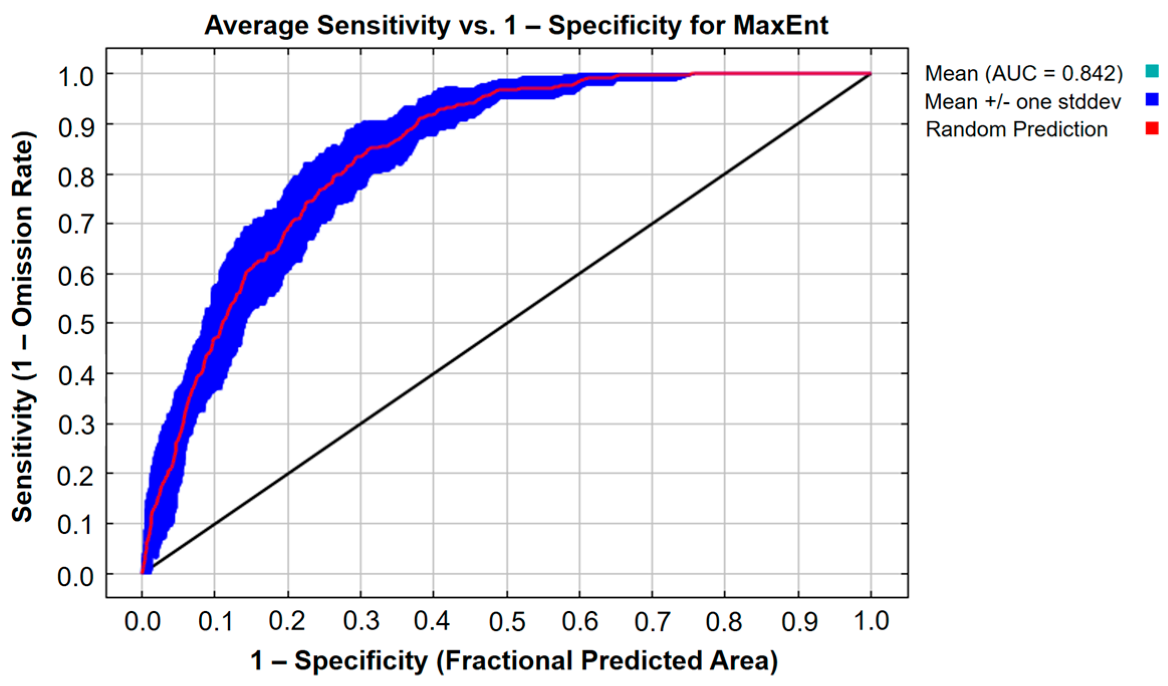
2.3.1. Validating Accuracy of MaxEnt

MaxEnt accuracy was evaluated using the area under the concentration-time curve (AUC) of the receiver operating characteristic Curve(ROC) curve. The ROC curve plots the percentage of correct and incorrect predictions of the true state of the target on the x- and y-axes, respectively; the lower the percentage of incorrect predictions, the higher the percentage of correct predictions, and the larger the area under the ROC curve, the better the model’s prediction [69].
AUC is widely used to compare the accuracy rates of various prediction models, and the accuracy value of the model obtained through it has the merit of being independent of the reference value. If the AUC value is 0.5 or less, the analysis of the model is judged to be meaningless; if it is 0.7 or more but less than 0.9, it is considered to have adequate performance, and if the AUC value is 0.9 or more and approaches 1.0, the analysis performance of the model is evaluated as excellent [70]. Thus, AUC is widely used to compare different models [71].
Additionally, the jackknife technique [72] was used to evaluate the main variables affecting the distribution of Monochamus alternatus. Jackknife is a resampling technique for estimating the variance of an estimate and is used in ecology to assess the reliability of phylogenetic trees for estimating population parameters or phylogenetic inferences [56]. Jackknife results indicate the importance of each variable in explaining whether a species is distributed by removing one of the total variables to create a new dataset [73].

2.3.2. Validating Accuracy of Ensemble

Kappa, AUC, and TSS values were used to validate the ensemble’s accuracy. The Kappa coefficient determines the overall accuracy of model predictions using the predictive accuracy expected by chance and helps assess accuracy by correcting for the possibility of classification matching by chance. Kappa is widely used for model validation in ecology, primarily for validating the accuracy of presence–absence data. In particular, it has been used to validate the accuracy of land-cover classifications using satellite imagery [73]. The value of the coefficient lies between −1 and 1, with the following implications: ˂0 “little agreement”; ˂0.4 “lower than moderate agreement”; 0.4–0.6 “moderate agreement”; 0.6–0.8 “high agreement”; ˃0.8 “near agreement.” Kappa provides a relatively simple selection criterion for evaluating binomial predictions. However, it is not independent of the criterion value, which makes it difficult to compare models [14].
The TSS compensates for Kappa’s lack of baseline independence while retaining the advantage of providing a baseline value for a binary variable, and the TSS results are highly correlated with the AUC, which is baseline-independent [74]. The range of the coefficient values was the same as that of Kappa [14].

3. Results

3.1. MaxEnt Prediction Results

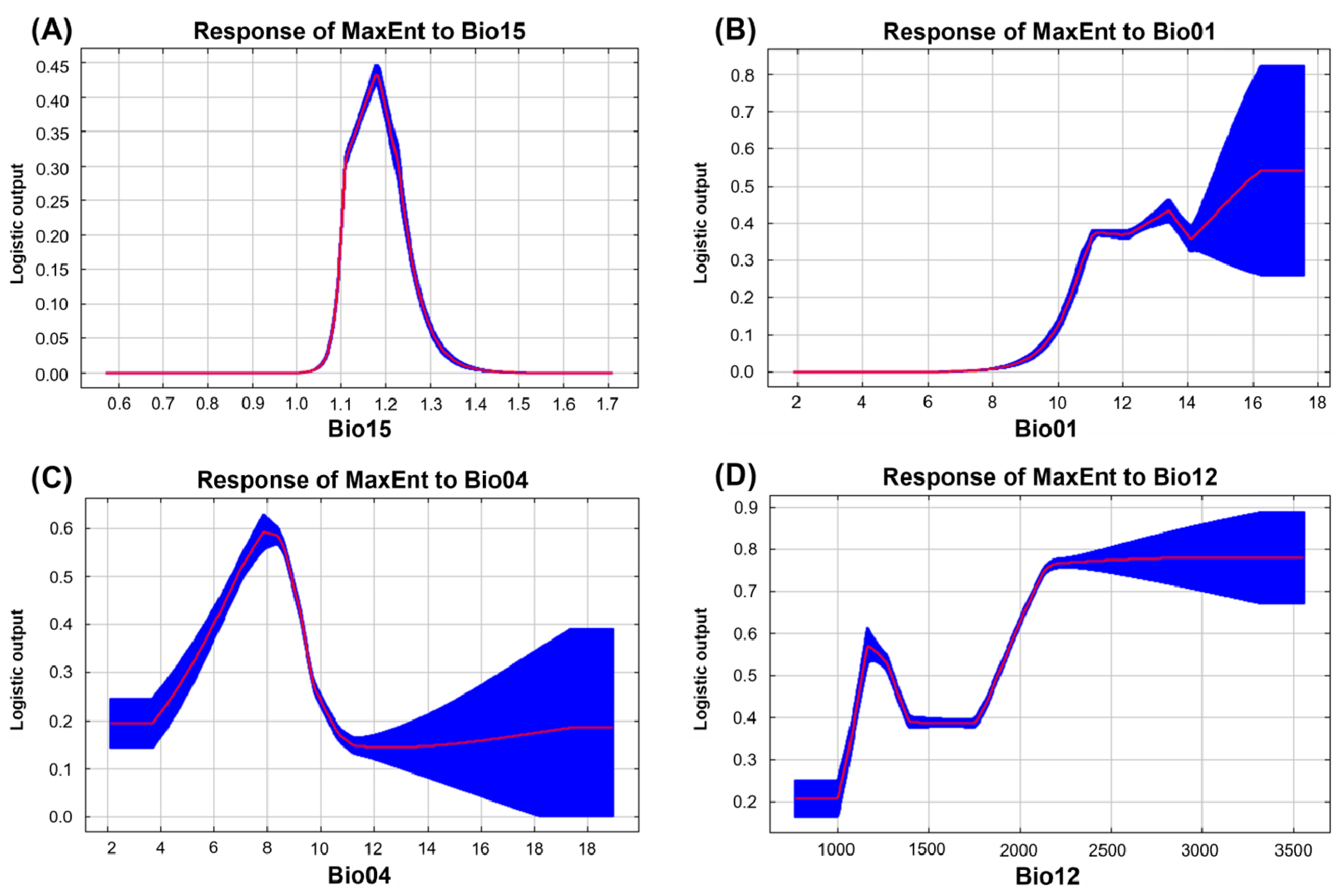
3.1.1. Evaluating Variables

A total of 1226 resampled Monochamus alternatus occurrence points and the EIs of the baseline period selected by Pearson Correlation Coefficient, terrain variables, and FTM were entered into the MaxEnt program and analyzed for their contribution and importance to potential habitats using 10 cross-validations.
As a result of checking the contribution, the variable affecting the distribution of Monochamus alternatus in South Korea was Bio15 (24.2%), and the average temperature of the driest quarter was confirmed to have the highest effect on the distribution, followed by Bio01 (22.7%), Bio04 (19.2%), and Bio12 (14.4%), and the importance of the variable was confirmed to be Bio15 (34.5%), Bio04 (17.6%), Bio01 (17.5%), and Bio12 (8.4%) (Appendix B, Table A2).
The response curves for Bio15, Bio01, Bio04, and Bio12, the variables with the highest contribution (>10%) to the distribution of Monochamus alternatus, showed that the probability of presence increased with increasing values of Bio09 and Bio04 and decreased after a certain point. Nevertheless, for Bio01 and Bio12, the probability of presence increased as the value increased (Figure 2).

3.1.2. Jackknife Validation

The Jackknife test was used to determine the relative importance of the variables, and Bio04 obtained the highest value, followed by Bio01, and Bio15 (Figure 3). Thus, temperature and precipitation strongly influence the distribution of Monochamus alternatus.

3.1.3. Evaluating Accuracy

After 10 iterations of cross-validation for the final selected LQHP_0.5 model, the AUC value was calculated to be 0.842, with a standard deviation of 0.012, which was considered a reliable model (Figure 4).

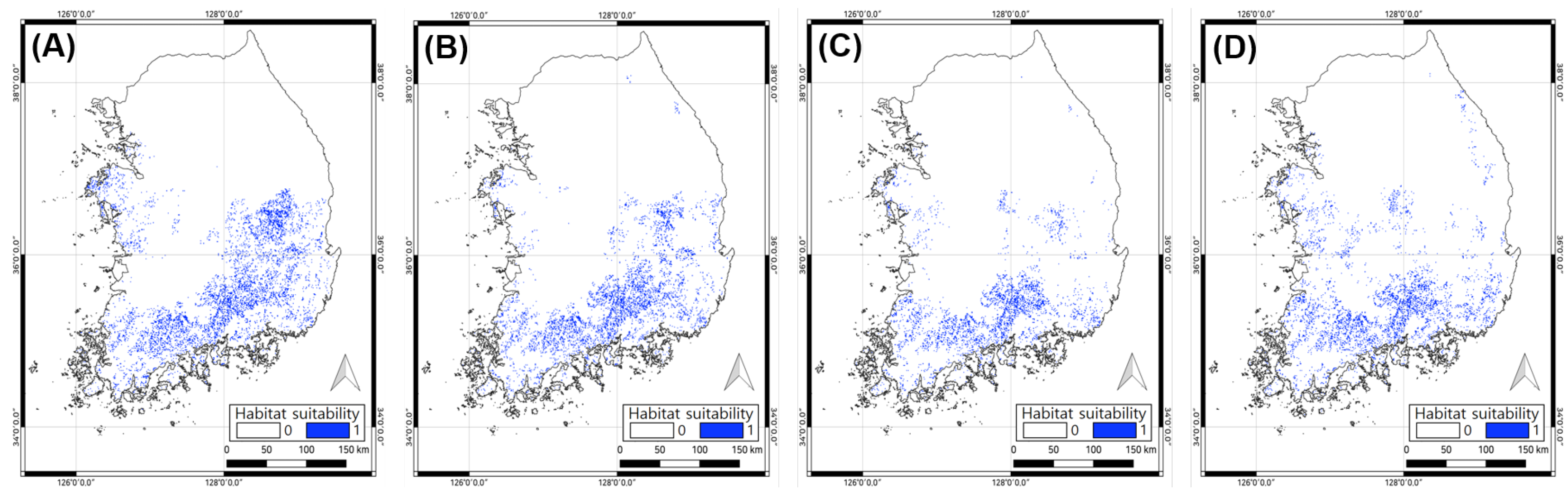
3.1.4. Potential Habitat Prediction

To determine the variability in the future potential habitats for Monochamus alternatus, a binary map with two values of potential habitat (1) and unsuitable habitat (0) was generated from the probability map (Figure 5 and Figure 6). The threshold value was calculated using the maximum training sensitivity and the specificity logistic threshold calculated after running MaxEnt [75]; the threshold was calculated to be 0.310. In a binary map, only areas with a threshold value above the threshold used in the habitat suitability model are implemented as potential habitats. The threshold is represented by calculating the sensitivity and specificity indices for the training data and is often used when the distribution of habitats is intuitively represented to determine the maximum habitat range of a species for conservation or invasive alien species [75].
The analysis showed that in the baseline period, a potential habitat for Monochamus alternatus was found in the southern part of South Korea, including Jeonnam, Gyeongnam, Daegu, Busan, Ulsan, and some areas of Gyeongbuk, with a potential habitat area of 4807 km2 (Appendix B, Table A5). When examining the variability of future potential habitats by scenario, the difference in distribution variability was not significant in the near future compared with the baseline period. Nevertheless, in both scenarios, the potential habitat for Monochamus alternatus was found in Gangwon, especially Gangneung and Inje city in northern South Korea. This indicates that Monochamus alternatus has moved northward under the influence of climate change. In the intermediate future, there will be an increase in the north of the existing distribution area, and it will be newly found in the Taean Peninsula and parts of the Taebaek Mountains. In the far future analysis, SSP2-4.5 showed a similar distribution pattern to that of SSP5-8.5 in the intermediate future, and in SSP5-8.5 of far future, most areas were found to be potential habitats for Monochamus alternatus except northern Gyeonggi (Figure 5 and Figure 6).
Looking at the potential habitat area by scenario, SSP2-4.5 in the near future was 4926 km2, a slight increase from the baseline period, while SSP5-8.5 showed a slight decrease to 4262 km2. In the intermediate future, the potential habitat area increased to 5942 km2 for SSP2-4.5, and 7278 km2 for SSP5-8.5, while in the far future, SSP2-4.5 was 7600 km2 and SSP5-8.5 was 11,345 km2. Both scenarios showed an increase in the potential habitat area, but the largest increase was observed under SSP5-8.5 (Appendix B, Table A5).

3.2. Ensemble Prediction Results

3.2.1. Evaluating Variables

Data from 1266 resampled Monochamus alternatus sites and 10 environmental variables constructed from monthly data from 1981 to 2010, the baseline period, were entered into an ensemble using the R package BIOMOD2, and five K-fold cross-validations were performed to analyze their importance as potential habitats for Monochamus alternatus.
Considering the importance of the variables in the ensemble, Bio02(0.240) had the greatest influence on the distribution of Monochamus alternatus, followed by Bio15 (0.202), Bio04 (0.196), and Bio01 (0.101) (Appendix B, Table A4). The variables Bio15, Bio04, and Bio01 were also found to be important in MaxEnt and the ensemble; however, in the ensemble, the variable Bio02 (mean diurnal variation) was estimated to be more important than the variable Bio12 (annual precipitation), which was found to be significant in MaxEnt.

3.2.2. Evaluating Accuracy

To build the ensemble, we used committee averaging of the EMca algorithm. The EMca algorithm converts the continuous probability distribution results of individual models selected with high accuracy into occurrence and non-occurrence data and superimposes them to derive a single average result [24,76]. In this study, we implemented the ensemble by weighting the TSS value of the individual model with 0.7 through the EMca algorithm. As a result of checking the accuracy of the model, Kappa was calculated to be 0.834, TSS was 0.843, and AUC was 0.921 (Figure 7), which was judged to be relatively superior to MaxEnt.

3.2.3. Potential Habitat Prediction

To determine the variability in future potential habitats for Monochamus alternatus, we utilized probability maps and converted them into binary maps. For this purpose, the threshold value at which the TSS value was maximized [65,74] was used and the threshold value was calculated to be 419. The analysis showed that the potential habitats of Monochamus alternatus in the baseline period were mainly found in Jeonnam, Gyeongnam, Gwangju, Daegu, Busan, Ulsan, Chungnam, and Gyeongbuk, but no potential habitats were found in areas with relatively high altitudes compared with other areas where potential habitats were predicted. The area of potential habitat in the base year was identified as 5477 km2 (Appendix B, Table A5).
Looking at the variability of future potential habitats by scenario, the near future did not show much difference in distribution variability compared with the baseline period, and, similar to MaxEnt, a potential habitat for Monochamus alternatus was found in Gangneung and Inje city of Gangwon. The intermediate future did not show significant variability compared with the near future, but it was found in mountainous areas that were not represented as potential habitats in the near future due to higher altitude, and SSP5-8.5 was found in parts of the Taebaek Mountains and Sokrisan National Park, as well as in Hwaseong City and Incheon, which were not found in SSP2-4.5. In the far future analysis, SSP2-4.5 showed a distribution pattern similar to that of SSP5-8.5 in the intermediate future, and the potential habitats of SSP5-8.5 increased in the Taean Peninsula, Kyeongbuk. Additionally, Gangwon showed a tendency to increase potential habitats centered on some urban areas on the east coast and Taebaek Mountains (Figure 8 and Figure 9).
When looking at potential habitat areas for the near, intermediate, and far futures by scenario, SSP2-4.5 showed decreases in the far future of 4862, 3811, and 3177 km2, respectively, and SSP5-8.5 showed decreases in the intermediate future and increases in the far future of 4318, 3136, and 4034 km2, respectively (Appendix B, Table A5).

3.3. Comparing MaxEnt and Ensemble Results

To compare the differences between MaxEnt and the ensemble, binary maps were nested and analyzed (Figure 10 and Figure 11). The nested results showed that the two models had similar distributions in the baseline period and the near future. However, both MaxEnts showed relative overestimation in the future. In particular, SSP5-8.5 of far future predicted a potential habitat for Monochamus alternatus in all target sites, except northern Gyeonggi, where pine forests are not distributed, suggesting the need for prevention and control measures for the whole of South Korea in the medium to long term.

4. Discussion

MaxEnts, reflecting both SSP2-4.5 and SSP5-8.5, showed a trend of spreading northward from the Chungnam region and along the Taebaek Mountains to Gangwon from the present to the far future. Both models showed potential habitats in Gangwon in the near future, and SSP5-8.5 predicted a larger area of potential habitat spread in the Taebaek Mountains and surrounding forests in the intermediate and far futures compared with SSP2-4.5. This is consistent with the characteristics of SSP5-8.5 [77], which assumed high fossil fuel use and expanded urban development.
For the ensemble reflecting SSP2-4.5, the near future showed a similar pattern to that of the present; nonetheless, the overall potential habitat area decreased in the far future. This reflects the SSP2-4.5 scenario, which maintains current emissions until 2050 and then decreases them. However, some potential habitat areas appeared in Gangwon, centered on the Taebaek Mountains, suggesting that Monochamus alternatus may expand northward in the future, mainly in pine forest communities.
In the case of the ensemble reflecting SSP5-8.5, the area of potential habitat decreased in the intermediate future and increased in the future. This trend occurred because the results of all eight models (GLM, GAM, etc.) overlapped.
In ensemble reflecting SSP5-8.5 of the far future, representative spread areas are Chungnam Taean, Gyeongbuk Uljin, and Gangwon Gangneung. Taean is home to the Chungnam Protected Species “Anmyeon Pine Forest” [78], Gyeongbuk Uljin’s Keumgang Pine Forest habitat is designated as a forest genetic protection area [79], and Gangwon’s Daegwallyeong Pine Forest is protected by the KFS as a protected forest [80]. In other words, climate change may increase the probability that pine forests with high protection values will be affected by PWD, and more systematic prevention and control measures are necessary in the medium to long term.
When the two models were nested, they showed similar distributions in the baseline and near future, but both scenarios showed a tendency to overestimate the far future MaxEnt, especially in Gyeongbuk and Gangwon. This is similar to previous studies [22,81,82,83,84] and some studies have attributed the overestimation to the uncertainty of the single model [21,85]. In particular, in SSP5-8.5, it was pronounced in Deogyusan National Park, Woraksan National Park, southern Gyeonggi, and the mountainous areas of Gangwon. Additionally, the potential habitat for MaxEnt reflecting SSP5-8.5 of the far future was predicted throughout South Korea, except northern Gyeonggi, where pine forests are not distributed. To resolve this overestimation tendency, it is necessary to improve the accuracy and reliability of predictions by reducing model uncertainty through collaborative research between field and model experts.
Furthermore, the concentration of potential habitats in Jeonnam, Gyungnam, and Gyoungbuk in all analyses is likely due to the fact that both MaxEnt and ensemble models are modeled by reflecting data on the occurrence points of this species [86].

5. Conclusions

This study was conducted as basic research to analyze the trend of PWD spread in South Korea due to climate change. To this end, we predicted the potential habitats of Monochamus alternatus, a representative vector insect that mainly inhabits southern South Korea. The climate change scenarios were SSP2-4.5 and SSP5-8.5, which compensated for the shortcomings of the existing RCP scenario and reflected the IPCC 6th report. For the SDM, the MaxEnt and the ensemble were compared and analyzed to determine the spread trend. Further, the FTM was added to the environmental variables to reflect the occurrence of PWD in Pinus thunbergii, Pinus densiflora, and Pinus koraiensis to ensure the reliability of the model.
In summary, both models confirmed that temperature and precipitation have a strong influence on the distribution of Monochamus alternatus. Moreover, the distribution area tends to move northward in the far future, and MaxEnt, reflecting SSP5-8.5, into the far future, analyzes the entire country as a potential habitat for the vector, except for northern Gyeonggi, where the distribution of pine forests is relatively small. Furthermore, the potential habitats analyzed included Taean, Uljin, and Gangneung, all of which are protected pine forests in South Korea, suggesting that special measures should be taken to prevent, detect, and control the disease throughout South Korea and in protected areas.
MaxEnt tends to overestimate the expansion, which is similar to the results of Ahn et al. (2015) [85] and Jung et al. (2020) [21]. Relatively speaking, the ensemble produced fewer predicted potential habitat areas than MaxEnt because it was created by nesting multiple models; however, when assessed for accuracy, the ensemble was more accurate than MaxEnt.
Although this study was conducted to prevent the spread of the disease in South Korea and to establish basic data for future conservation plans and preventive measures in potentially affected areas of PWD, it is believed that expanding the study area to the entirety of South Korea could also contribute to providing basic data for related fields in North Korea, where pine forests are dominant among coniferous forests [87], and where PWD control technologies are relatively underdeveloped [88].
A limitation of this study is that MaxEnt tended to overestimate the predicted range compared with the ensemble. We believe that optimized model implementation through collaborative research between field and model experts on the causes and consequences of uncertainty could lead to more accurate predictions of potential habitats for Monochamus alternatus in the future.

Author Contributions

Conceptualization, S.-W.K.; Methodology, S.-W.K.; Validation, S.-W.K.; Data interpretation, S.-W.K.; Writing—review & editing, S.-W.K.; Software, B.-J.J. and M.-G.L.; Literature search, B.-J.J. and M.-G.L.; Resources, B.-J.J.; Visualization, B.-J.J.; Data analysis, B.-J.J.; Formal analysis, M.-G.L.; Writing—original draft, M.-G.L. All authors have read and agreed to the published version of the manuscript.

Funding

This Study was supported by the 2023 research fund from Wonkwang University.

Data Availability Statement

Restrictions apply to the availability of these data. ‘Detailed climate change scenario data for agricultural applications, based on the SSP scenario’ and ‘GPS points of PWD-affected trees’ are available with permission from the Rural Development Administration and Korea Forestry Promotion Institute, respectively.

Conflicts of Interest

The authors declare no conflict of interest.

Appendix A

Table A1. List of EIs (O’Donnell and Ignizio, 2012).
SeparationDescriptionCategorization
Bio01Average annual temperature°C
Bio02Average diurnal range°C
Bio03Isothermal%
Bio04Temperature seasonality (standard deviation)°C
Bio04aTemperature Seasonality (CV)%
Bio05Highest temperature in the warmest month°C
Bio06Minimum temperature in the coldest month°C
Bio07Annual temperature range °C
Bio08Average temperature in the wettest quarter°C
Bio09Average temperature in the driest quarter°C
Bio10Average temperature in the warmest quarter°C
Bio11Average temperature in the coldest quarter°C
Bio12Annual precipitationmm
Bio13Precipitation in the wettest monthmm
Bio14Precipitation in the driest monthsmm
Bio15Precipitation seasonality%
Bio16Wettest quarter precipitationmm
Bio17Dryest quarter precipitationmm
Bio18Warmest quarter precipitationmm
Bio19Coldest quarter precipitationmm

Appendix B

Table A2. Results of Pearson correlation analysis of climate variables.
Bio01Bio02Bio03Bio04Bio04aBio05Bio06Bio07Bio08Bio09Bio10Bio11Bio12Bio13Bio14Bio15Bio16Bio17Bio18Bio19
1.000−0.414−0.132−0.733−0.7690.9000.961−0.7850.8250.9380.8880.967−0.219−0.264−0.010−0.316−0.3400.088−0.4210.164
1.0000.9200.7200.710−0.067−0.5260.687−0.035−0.535−0.061−0.5340.1660.251−0.3880.4010.295−0.3880.303−0.372
1.0000.4080.3930.129−0.2070.3640.129−0.2160.124−0.2190.1160.145−0.3840.2030.179−0.3160.158−0.262
1.0000.999−0.377−0.8840.995−0.253−0.902−0.345−0.8800.1170.291−0.3040.6260.337−0.4510.416−0.523
1.000−0.426−0.9080.998−0.304−0.922−0.395−0.9040.1290.296−0.2840.6130.345−0.4290.425−0.502
1.000−0.764−0.4520.9540.7230.9970.771−0.208−0.167−0.197−0.056−0.243−0.139−0.317−0.073
1.000−0.9210.6570.9900.7410.999−0.188−0.2920.117−0.472−0.3610.248−0.4540.329
1.000−0.331−0.933−0.422−0.9150.1350.303−0.2820.6180.353−0.4270.436−0.500
1.0000.5980.9660.668−0.286−0.199−0.2520.045−0.261−0.258−0.276−0.240
1.0000.6970.989−0.158−0.2790.181−0.523−0.3500.325−0.4470.413
1.0000.749−0.208−0.161−0.200−0.030−0.234−0.157−0.299−0.100
1.000−0.191−0.2900.108−0.456−0.3590.234−0.4480.315
1.0000.9010.3500.2560.9440.4060.8760.451
1.0000.1120.5780.9730.1230.9130.153
1.000−0.5530.1290.9510.1320.861
1.0000.542−0.6460.569−0.645
1.0000.1450.9640.171
1.0000.1000.970
1.0000.092
1.000
Table A3. Contribution and Importance of each variable in the MaxEnt.
VariableContribution (%)Importance (%)
Bio0122.717.5
Bio024.97.9
Bio0419.217.6
Bio1214.48.4
Bio142.45.7
Bio1524.234.5
Aspect3.33.4
Slope0.90.8
DEM4.33.3
FTM3.80.8
Table A4. Importance of each variable in the ensemble.
VariableImportance (%)
Bio010.101
Bio020.240
Bio040.196
Bio120.079
Bio140.038
Bio150.202
Aspect0.046
Slope0.018
DEM0.029
FTM0.005
Table A5. Potential Habitat Area of the MaxEnt and ensemble.
MaxEntEnsemble
SeparationYearArea (km2)YearArea (km2)
Baseline Period1981 to 201048071981 to 20105477
SSP2-4.52011 to 204049262011 to 20404862
2041 to 207059422041 to 20703811
2071 to 210076002071 to 21003177
SSP5-8.52011 to 204042622011 to 20404318
2041 to 207072782041 to 20703136
2071 to 210011,3452071 to 21004034

References

  1. Zhao, B.G.; Futai, K.; Sutherland, J.R.; Takeuchi, Y. Pine Wilt Disease; Springer: Tokyo, Japan, 2008. [Google Scholar]
  2. Linit, M.J. Nematode-vector relationships in the pine wilt disease system. J. Nematol. 1988, 20, 227. [Google Scholar] [PubMed]
  3. Yi, C.K.; Byun, B.H.; Park, J.D.; Yang, S.I.; Chang, K.H. First finding of the pine wood nematode, Bursaphelenchus xylophilus (Steiner et Buhrer) Nickle, and its insect vector in Korea. Res. Rep. For. Res. Inst. 1989, 38, 141–149. [Google Scholar]
  4. Kang, D.I.; Son, S.C.; Yu, S.M.; Lee, B.Y.; Park, Y.S. 2022 Statistical Yearbook of Forestry. Available online: https://kfss.forest.go.kr/stat/ptl/fyb/frstyYrBookList.do?curMenu=9854 (accessed on 10 December 2022).
  5. Lu, Q.; Wang, W.; Liang, J. Potential suitability assessment of Bursaphelenchus xylophilus in China. For. Res. Chin. Acad. For. 2005, 18, 460. [Google Scholar]
  6. Lee, M.G.; Cho, H.B.; Youm, S.K.; Kim, S.W. Detection of pine wilt disease using time series UAV imagery and deep learning semantic segmentation. Forests 2023, 14, 1576. [Google Scholar] [CrossRef]
  7. Futai, K. Pine wilt in Japan: From first incidence to the present. In Pine Wilt Disease; Springer: Tokyo, Japan, 2008; pp. 5–12. [Google Scholar]
  8. Hirata, A.; Nakamura, K.; Nakao, K.; Kominami, Y.; Tanaka, N.; Ohashi, H.; Matsui, T. Pine wilt disease. J. For. Res. 2008, 13, 3–11. [Google Scholar]
  9. Kim, J.B.; Kim, D.Y.; Park, N.C. Development of aerial precision monitoring techniques for pine wilt disease using GIS and GPS. J. Korean Soc. Geospat. Inf. Sci. 2010, 13, 28–34. [Google Scholar]
  10. Kim, M.J.; Bang, H.S.; Lee, J.W. Monitoring techniques for the leading edge of pine wilt disease using unmanned aerial vehicles: Focused on Sejong City. J. Korean For. Soc. 2017, 106, 100–109. [Google Scholar]
  11. Jung, C.S.; Jeong, Y.J.; Moon, I.S.; Han, H.R.; Ko, S.H.; Choi, K.S.; Kim, K.H.; Lim, J.H.; Yang, H.M.; Shin, H.C.; et al. Research on the Ecological Characteristics of Pine Wilt Disease; Korea Forest Research Institute: Seoul, Republic of Korea, 2009. [Google Scholar]
  12. Wilson, J.W.; Sexton, J.O.; Jobe, R.T.; Haddad, N.M. The relative contribution of terrain, land cover, and vegetation structure indices to species distribution models. Biol. Conserv. 2013, 164, 170–176. [Google Scholar] [CrossRef]
  13. Crimmins, S.M.; Dobrowski, S.Z.; Mynsberge, A.R. Evaluating ensemble forecasts of plant species distributions under climate change. Ecol. Model. 2013, 266, 126–130. [Google Scholar] [CrossRef]
  14. Franklin, J. Mapping Species Distributions: Spatial Inference and Prediction; Cambridge University Press: Cambridge, UK, 2010. [Google Scholar]
  15. Thorn, J.S.; Nijman, V.; Smith, D.; Nekaris, K.A.I. Ecological niche modelling as a technique for assessing threats and setting conservation priorities for Asian slow lorises (Primates: Nycticebus). Divers. Distrib. 2009, 15, 289–298. [Google Scholar] [CrossRef]
  16. Venette, R. Pest Risk Modeling and Mapping for Invasive Alien Species; CABI: Wallingford, UK, 2015; pp. 1–17. [Google Scholar]
  17. Pearson, R.G.; Raxworthy, C.J.; Nakamura, M.; Townsend Peterson, A. Predicting species distributions from small numbers of occurrence records: A test case using cryptic geckos in Madagascar. J. Biogeogr. 2007, 34, 102–117. [Google Scholar] [CrossRef]
  18. Berger, A.; Della Pietra, S.A.; Della Pietra, V.J. A maximum entropy approach to natural language processing. Comput. Linguist. 1996, 22, 39–71. [Google Scholar]
  19. Phillips, S.J.; Anderson, R.P.; Schapire, R.E. Maximum entropy modeling of species geographic distributions. Ecol. Model. 2006, 190, 231–259. [Google Scholar] [CrossRef]
  20. Kwon, H.S. Application of ensemble models for uncertainty assessment of species distribution models. J. Korean Assoc. Geogr. Inf. Stud. 2014, 22, 47–52. [Google Scholar]
  21. Jung, H.I.; Choi, Y.Y.; Ryu, J.E.; Jeon, S.W. Accuracy evaluation of predicted distribution of Pinus koraiensis potential habitats using species distribution models-Verification of ensemble methodology. J. Korean Soc. Clim. Change Res. 2020, 11, 37–51. [Google Scholar]
  22. Araújo, M.B.; Whittaker, R.J.; Ladle, R.J.; Erhard, M. Reducing uncertainty in projections of extinction risk from climate change. Glob. Ecol. Biogeogr. 2005, 14, 529–538. [Google Scholar] [CrossRef]
  23. Thuiller, W.; Lafourcade, B.; Engler, R.; Araújo, M.B. BIOMOD-a platform for ensemble forecasting of species distributions. Ecography 2009, 32, 369–373. [Google Scholar] [CrossRef]
  24. Meller, L.; Cabeza, M.; Pironon, S.; Barbet-Massin, M.; Maiorano, L.; Georges, D.; Thuiller, W. Ensemble distribution models in conservation prioritization: From consensus predictions to consensus reserve networks. Divers. Distrib. 2014, 20, 309–321. [Google Scholar] [CrossRef] [PubMed]
  25. Lee, D.S.; Choi, W.I.; Nam, Y.; Park, Y.S. Predicting potential occurrence of pine wilt disease based on environmental factors in South Korea using machine learning algorithms. Ecol. Inform. 2021, 64, 101378. [Google Scholar] [CrossRef]
  26. Choi, H.J. Predicting the Geographical Distribution of Pine Wilt Disease and Oak Wilt Disease under Climate Change Scenarios. Master’s Thesis, Gyeongsang National University, Graduate School, Jinju-si, Republic of Korea, 2019. [Google Scholar]
  27. Hirata, A.; Nakamura, K.; Nakao, K.; Kominami, Y.; Tanaka, N.; Ohashi, H.; Takenaka Takano, K.; Takeuchi, W.; Matsui, T. Potential distribution of pine wilt disease under future climate change scenarios. PLoS ONE 2017, 12, e0182837. [Google Scholar] [CrossRef]
  28. Kim, J.W.; Jeong, H.C.; Park, Y.H. Predicting the potential distribution of Monochamus alternatus under climate change. Korean J. Appl. Entomol. 2016, 55, 501–511. [Google Scholar] [CrossRef]
  29. Arguez, A.; Vose, R.S. The definition of the standard WMO climate normal: The key to deriving alternative climate normals. Bull. Am. Meteorol. Soc. 2011, 92, 699–704. [Google Scholar] [CrossRef]
  30. Buisson, L.; Thuiller, W.; Casajus, N.; Lek, S.; Grenouillet, G. Uncertainty in ensemble forecasting of species distribution. Glob. Chang. Biol. 2010, 16, 1145–1157. [Google Scholar] [CrossRef]
  31. Korea Forestry Promotion Institute. 2023. Available online: https://namudr.kofpi.or.kr (accessed on 12 December 2022).
  32. Jung, Y.Y.; Kim, S.W. A Study on the UAV-based vegetable index comparison for detection of pine wilt disease trees. J. Cadastre Land InformatiX 2020, 50, 201–214. [Google Scholar]
  33. Yackulic, C.B.; Chandler, R.; Zipkin, E.F.; Royle, J.A.; Nichols, J.D.; Campbell Grant, E.H.; Veran, S. Presence-only modelling using MAXENT: When can we trust the inferences? Methods Ecol. Evol. 2013, 4, 236–243. [Google Scholar] [CrossRef]
  34. Xu, T.; Hutchinson, M. ANUCLIM Version 6.1 User Guide; The Australian National University, Fenner School of Environment and Society: Acton, Australia, 2011. [Google Scholar]
  35. Kriticos, D.J.; Webber, B.L.; Leriche, A.; Ota, N.; Macadam, I.; Bathols, J.; Scott, J.K. CliMond: Global high-resolution historical and future scenario climate surfaces for bioclimatic modelling. Methods Ecol. Evol. 2012, 3, 53–64. [Google Scholar] [CrossRef]
  36. Karger, D.N.; Conrad, O.; Böhner, J.; Kawohl, T.; Kreft, H.; Soria-Auza, R.W.; Kessler, M. Climatologies at high resolution for the earth’s land surface areas. Sci. Data 2017, 4, 170122. [Google Scholar] [CrossRef]
  37. Shim, G.M.; Kim, Y.S.; Heo, J.N.; Kang, M.G.; Jo, S.R.; Choi, W.J. A Technical Guide for Producing Detailed Climate Change Scenario Data for Agricultural Applications. Available online: https://www.korea.kr/archive/expDocView.do?docId=39829 (accessed on 13 December 2022).
  38. Heikkinen, R.K.; Luoto, M.; Araújo, M.B.; Virkkala, R.; Thuiller, W.; Sykes, M.T. Methods and uncertainties in bioclimatic envelope modeling under climate change. Prog. Phys. Geogr. 2006, 30, 751–777. [Google Scholar] [CrossRef]
  39. Dormann, C.F.; Elith, J.; Bacher, S.; Buchmann, C.; Carl, G.; Carré, G.; Lautenbach, S. Collinearity: A review of methods to deal with it and a simulation study evaluating their performance. Ecography 2013, 36, 27–46. [Google Scholar] [CrossRef]
  40. Kumar, S.; Stohlgren, T.J. Maxent modeling for predicting suitable habitat for threatened and endangered tree Canacomyrica monticola in New Caledonia. J. Ecol. Nat. Environ. 2009, 1, 94–98. [Google Scholar]
  41. Padalia, H.; Srivastava, V.; Kushwaha, S.P.S. Modeling potential invasion range of alien invasive species, Hyptis suaveolens (L.) Poit. in India: Comparison of MaxEnt and GARP. Ecol. Inform. 2014, 22, 36–43. [Google Scholar] [CrossRef]
  42. Negrini, M.; Fidelis, E.G.; Picanço, M.C.; Ramos, R.S. Mapping of the Steneotarsonemus spinki invasion risk in suitable areas for rice (Oryza sativa) cultivation using MaxEnt. Exp. Appl. Acarol. 2020, 80, 445–461. [Google Scholar] [CrossRef] [PubMed]
  43. Jo, N.H.; Kim, E.S.; Lee, B.R.; Lim, J.H. Prediction of potential distribution of pine trees using the MaxEnt model and analysis of the relationship with environmental variables. Proc. Korean Soc. Agric. For. Meteorol. 2019, 274, 47–56. [Google Scholar]
  44. Kim, H.M.; Kim, C.-Y.; Cho, J.-P.; Heo, J.-N.; Song, W.K. Prediction of Acer pictum subsp. mono Distribution using Bioclimatic Predictor Based on SSP Scenario Detailed Data. Ecol. Resilient Infrastruct. 2022, 9, 163–173. [Google Scholar]
  45. Kiyohara, T.; Suzuki, K.; Hashimoto, H. Population dynamics of Bursaphelenchus lignicolus at the early stage after inoculation. Trans. Annu. Meet. Jpn. For. Soc. 1975, 86, 299–300. [Google Scholar]
  46. Son, M.H.; Lee, W.K.; Lee, S.H.; Jo, H.G.; Lee, J.H. Natural dispersion analysis of pine wilt disease damage by spatial statistical methods. J. Korean For. Soc. 2006, 95, 240–249. [Google Scholar]
  47. Park, W.H.; Go, D.W.; Kwon, T.S.; Nam, Y.W.; Kwon, Y.D. Analysis of Pinewood Nematode Damage Expansion in Gyeonggi Province Based on Monitoring Data from 2008 to 2015. J. Korean For. Soc. 2018, 107, 486–496. [Google Scholar]
  48. CGIAR-CSI.CGIAR Consortium for Spatial Information. 2023. Available online: https://srtm.csi.cgiar.org/ (accessed on 21 November 2022).
  49. Korea Forest Service. National Forest Information System. 2023. Available online: https://www.forest.go.kr/newkfsweb/html/HtmlPage.do?pg=/fgis/UI_KFS_5002_020100.html&mn=KFS_02_04_03_04_01&orgId=fgis (accessed on 10 November 2022).
  50. Jeon, H.M.; Moon, I.S.; Heo, H.S.; Lee, S.G.; Park, N.C. Breaking News of Forest Science; Korea Forest Research Institute: Seoul, Republic of Korea, 2009. [Google Scholar]
  51. Kim, D.S.; Kwon, T.H.; Kim, J.M.; Lee, S.G.; Park, Y.B. Oviposition of Dendroctonus valens on Pinus densiflora and Larix leptolepis infested and uninfested logs. In Proceedings of the 2016 Annual Meeting and International Symposium of the Korean Society of Applied Entomology, Jeju-si, Republic of Korea, 25–26 April 2016; p. 71. [Google Scholar]
  52. Korea Forest Service. 2023. Available online: https://map.forest.go.kr/forest/ (accessed on 5 November 2022).
  53. Elith, J.; Phillips, S.J.; Hastie, T.; Dudík, M.; Chee, Y.E.; Yates, C.J. A statistical explanation of MaxEnt for ecologists. Divers. Distrib. 2011, 17, 43–57. [Google Scholar] [CrossRef]
  54. Zhong, X.; Zhang, L.; Zhang, J.; He, L.; Sun, R. Maxent Modeling for Predicting the Potential Geographical Distribution of Castanopsis carlesii under Various Climate Change Scenarios in China. Forests 2023, 14, 1397. [Google Scholar] [CrossRef]
  55. Grendár, J.M.; Grendár, M. Maximum entropy: Clearing up mysteries. Entropy 2001, 3, 58–63. [Google Scholar] [CrossRef]
  56. Phillips, S.J.; Dudík, M.; Schapire, R.E. A maximum entropy approach to species distribution modeling. In Proceedings of the Twenty-First International Conference on Machine Learning, Banff Alberta, AB, Canada, 4–8 July 2004; p. 83. [Google Scholar]
  57. Chen, S.; You, C.; Zhang, Z.; Xu, Z. Predicting the Potential Distribution of Quercus oxyphylla in China under Climate Change Scenarios. Forests 2024, 15, 1033. [Google Scholar] [CrossRef]
  58. Townsend Peterson, A.; Papeş, M.; Eaton, M. Transferability and model evaluation in ecological niche modeling: A comparison of GARP and Maxent. Ecography 2007, 30, 550–560. [Google Scholar] [CrossRef]
  59. Phillips, S.J.; Dudik, M. Modeling of species distributions with MaxEnt: New extensions and a comprehensive evaluation. Ecography 2008, 31, 161–175. [Google Scholar] [CrossRef]
  60. Kim, N.S.; Lee, H.C.; Cha, J.Y. Study on the change of plant seasons and spatial distribution characteristics using MODIS satellite images. J. Korean Soc. Environ. Restor. Technol. 2013, 16, 59–69. [Google Scholar] [CrossRef]
  61. Song, W.K. Habitat analysis of Hyla suweonensis in the breeding season using species distribution modeling. J. Korean Soc. Environ. Restor. Technol. 2015, 18, 71–82. [Google Scholar] [CrossRef]
  62. Morales, N.S.; Fernández, I.C.; Baca-González, V. MaxEnt’s parameter configuration and small samples: Are we paying attention to recommendations? A systematic review. PeerJ 2017, 18, e3093. [Google Scholar] [CrossRef]
  63. Oh, Y.J.; Kim, M.H.; Choi, S.G.; Kim, M.K.; Uh, J.W.; Yeop, S.J.; Bang, J.H.; Lee, Y.H. Predicting suitable habitats for Peromyscus maniculatus under SSPs scenarios. Ecol. Resilient Infrastruct. 2021, 8, 154–163. [Google Scholar]
  64. Warren, D.L.; Seifert, S.N. Ecological niche modeling in Maxent: The importance of model complexity and the performance of model selection criteria. Ecol. Appl. 2011, 21, 335–342. [Google Scholar] [CrossRef]
  65. Barbet-Massin, M.; Jiguet, F.; Albert, C.H.; Thuiller, W. Selecting pseudo-absences for species distribution models: How, where and how many? Methods Ecol. Evol. 2012, 3, 327–338. [Google Scholar] [CrossRef]
  66. Gigović, L.; Pourghasemi, H.R.; Drobnjak, S.; Bai, S. Testing a new ensemble model based on SVM and random forest in forest fire susceptibility assessment and its mapping in Serbia’s Tara National Park. Forests 2019, 10, 408. [Google Scholar] [CrossRef]
  67. Latif, Q.S.; Saab, V.A.; Dudley, J.G.; Hollenbeck, J.P. Ensemble modeling to predict habitat suitability for a large-scale disturbance specialist. Ecol. Evol. 2013, 3, 4348–4364. [Google Scholar] [CrossRef]
  68. Elith, J.; Graham, C.H.; Anderson, R.P.; Dudík, M.; Ferrier, S.; Guisan, A.; Zimmermann, N.E. Novel methods improve prediction of species’ distributions from occurrence data. Ecography 2006, 29, 129–151. [Google Scholar] [CrossRef]
  69. Tasche, D. Validation of internal rating systems and PD estimates. arXiv 2006, arXiv:physics/0606071. [Google Scholar]
  70. Hanley, J.A.; McNeil, B.J. The meaning and use of the area under a receiver operating characteristic (ROC) curve. Radiology 1982, 143, 29–36. [Google Scholar] [CrossRef] [PubMed]
  71. Seo, C.W.; Park, Y.R.; Choi, Y.S. Comparison study of biological species distribution models according to types of location data. J. Korean Spat. Inf. Soc. 2008, 16, 59–64. [Google Scholar]
  72. Quenouille, M.H. Approximate tests of correlation in time-series 3. In Mathematical Proceedings of the Cambridge Philosophical Society; Cambridge University Press: Cambridge, UK, 1949; Volume 45, pp. 483–484. [Google Scholar] [CrossRef]
  73. Wu, C.F.J. Jackknife, bootstrap and other resampling methods in regression analysis. Ann. Stat. 1986, 14, 1261–1295. [Google Scholar] [CrossRef]
  74. Allouche, O.; Tsoar, A.; Kadmon, R. Assessing the accuracy of species distribution models: Prevalence, Kappa and the true skill statistic (TSS). J. Appl. Ecol. 2006, 43, 1223–1232. [Google Scholar] [CrossRef]
  75. Liu, C.; White, M.; Newell, G. Selecting thresholds for the prediction of species occurrence with presence-only data. J. Biogeogr. 2013, 40, 778–789. [Google Scholar] [CrossRef]
  76. Hao, T.; Elith, J.; Guillera-Arroita, G.; Lahoz-Monfort, J.J. A review of evidence about use and performance of species distribution modeling ensembles like BIOMOD. Divers. Distrib. 2019, 25, 839–852. [Google Scholar] [CrossRef]
  77. O’Neill, B.C.; Kriegler, E.; Riahi, K.; Ebi, K.L.; Hallegatte, S.; Carter, T.R.; Marthur, R.; van Vuuren, D.P. A new scenario framework for climate change research: The concept of shared socioeconomic pathways. Clim. Change 2014, 122, 387–400. [Google Scholar] [CrossRef]
  78. Yonhap News. Chungnam Province Launches Campaign to Prevent Pine Wilt Disease in Taean. 2021. Available online: https://www.yna.co.kr/view/AKR20210307012800063 (accessed on 12 May 2024).
  79. Asia Economy. Forest Service starts emergency recovery of ‘Uljin Geumgang Pine Forest’ damaged by heavy snowfall. 2024. Available online: https://view.asiae.co.kr/article/2024032207542853226 (accessed on 24 May 2024).
  80. GlobalE. [Global E-Photo] Premium Forest <2> Gangneung Daegwallyeong Pine Forest… 100-Year-Old Geumgang Pine Colony. 2021. Available online: https://www.globale.co.kr/news/articleView.html?idxno=13813 (accessed on 24 May 2024).
  81. Thuiller, W.; Miguel, B.; Araújo, M.B.; Richard, G.; Pearson, R.W.; Lluis, B.; Sandra, L. Biodiversity conservation: Uncertainty in predictions of extinction risk. Nature 2004, 427, 145–148. [Google Scholar]
  82. Pearson, R.G.; Thuiller, W.; Araújo, M.B.; Martinez-Meyer, E.B.; Lluls, M.; Colin, M.; Lera, S.; Pedro, D.; Terence, P.; Lees, D.C. Model-based uncertainty in species range prediction. J. Biogeogr. 2006, 33, 1704–1711. [Google Scholar] [CrossRef]
  83. Elith, J.; Graham, C.H. Do they? How do they? WHY do they differ? On finding reasons for differing performances of species distribution models. Ecography 2009, 32, 66–77. [Google Scholar] [CrossRef]
  84. Miller, J.A. Virtual species distribution models: Using simulated data to evaluate aspects of model performance. Prog. Phys. Geogr. 2014, 38, 117–128. [Google Scholar] [CrossRef]
  85. Ahn, Y.J.; Lee, D.G.; Kim, H.G.; Park, C.; Kim, J.Y.; Kim, J.W. Predicting the distribution of suitable habitats for future Korean pine trees considering uncertainty. Korean Environ. Res. Technol. 2015, 3, 51–64. [Google Scholar]
  86. Lee, S.J.; Shin, D.B.; Lee, A.R.; Song, J.S.; Lim, C.H.; Oh, S.H. Analysis of the characteristics of dead pine trees and prediction of risk areas in the Wangpicheon Ecological Landscape Conservation Area: Focusing on the comparison between ensemble models and the MaxEnt model. Proc. Korean Soc. Environ. Ecol. 2022, 2, 49. [Google Scholar]
  87. Korea Forestry Promotion Institute. Advanced Information on Mountain Soil in North Korea and Selection of Suitable Afforestation Species; Korea Forestry Promotion Institute: Seoul, Republic of Korea, 2016; p. 78. [Google Scholar]
  88. Yonhap News Agency. Full-scale South-North Forest Cooperation through Joint Pine Wilt Disease Control and Modernization of 10 Nurseries. 2018. Available online: https://www.yna.co.kr/view/AKR20181022171200063 (accessed on 25 May 2024).
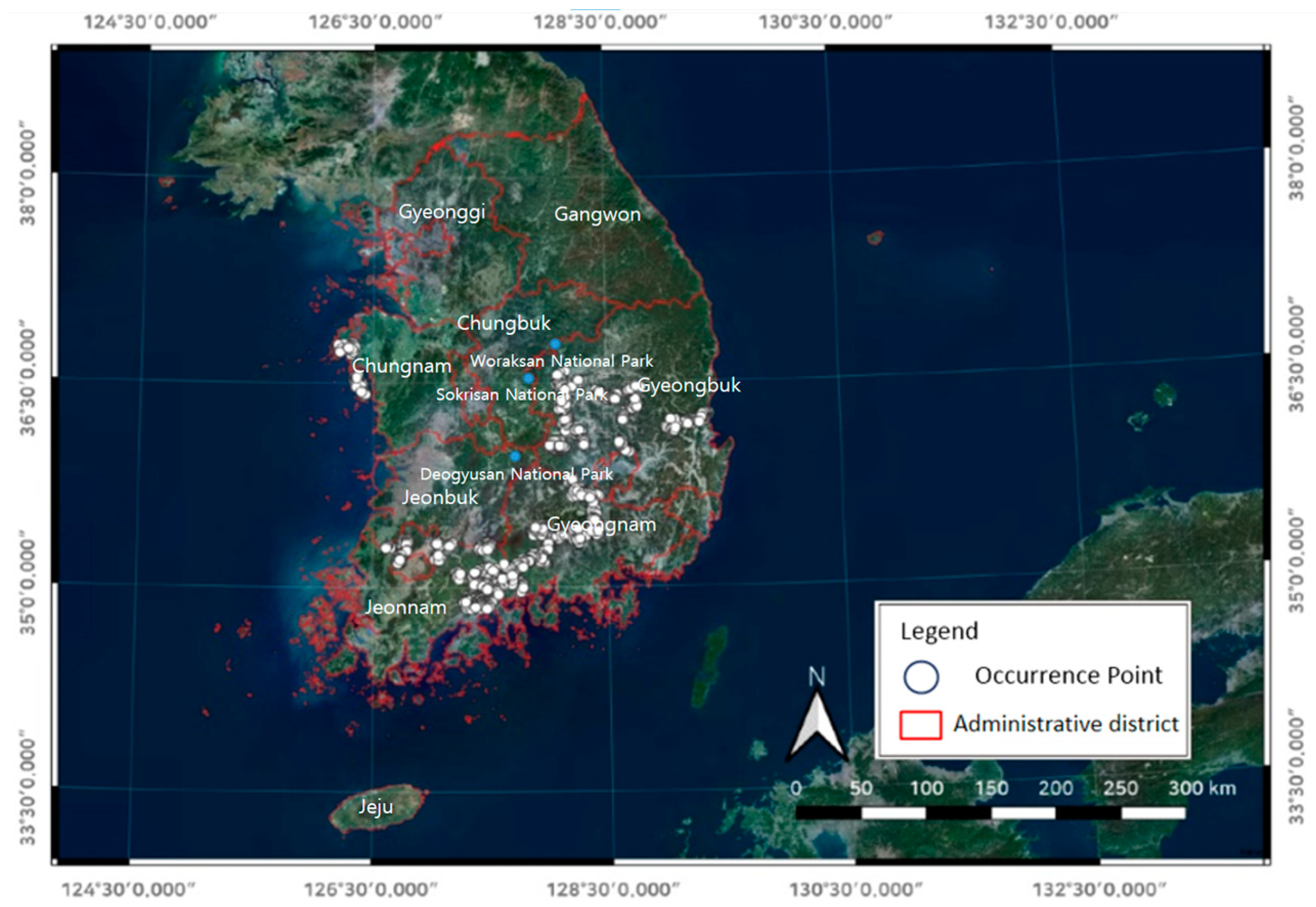
Figure 1. Resampling results for Monochamus alternatus occurrence points.
Forests 15 01563 g001
Figure 2. MaxEnt key-variable response graph (A) Bio15, (B) Bio01, (C) Bio04 and (D) Bio12.
Forests 15 01563 g002
Figure 3. MaxEnt Jackknife validation results.
Forests 15 01563 g003
Figure 4. MaxEnt model AUC values.
Forests 15 01563 g004
Figure 5. MaxEnt binary maps of SSP2-4.5 [(A) Baseline Period (1981–2010), (B) Near Future (2011–2040), (C) Intermediate Future (2041–2070) and (D) Far Future (2071–2100)].
Forests 15 01563 g005
Figure 6. MaxEnt binary maps of SSP5-8.5 [(A) Baseline Period (1981–2010), (B) Near Future (2011–2040), (C) Intermediate Future (2041–2070) and (D) Far Future (2071–2100)].
Forests 15 01563 g006
Figure 7. Ensemble Kappa, TSS and AUC values.
Forests 15 01563 g007
Figure 8. Ensemble binary maps of SSP2-4.5 [(A) Baseline Period (1981–2010), (B) Near Future (2011–2040), (C) Intermediate Future (2041–2070) and (D) Far Future (2071–2100)].
Forests 15 01563 g008
Figure 9. Ensemble binary maps of SSP5-8.5 [(A) Baseline Period (1981–2010), (B) Near Future (2011–2040), (C) Intermediate Future (2041–2070) and (D) Far Future (2071–2100)].
Forests 15 01563 g009
Figure 10. Model nesting maps of SSP2-4.5 [(A) Baseline Period (1981–2010), (B) Near Future (2011–2040), (C) Intermediate Future (2041–2070) and (D) Far Future (2071–2100)].
Forests 15 01563 g010
Figure 11. Model nesting maps of SSP5-8.5 [(A) Baseline Period (1981–2010), (B) Near Future (2011–2040), (C) Intermediate Future (2041–2070) and (D) Far Future (2071–2100)].
Forests 15 01563 g011
Table 1. Monochamus alternatus occurrence points.
OrderRegionOccurrence Points
1Gyeongnam3902
2Gyeongbuk5555
3Gwangju221
4Daegu429
5Jeonnam9282
6Chungnam1125
Total20,514
Disclaimer/Publisher’s Note: The statements, opinions and data contained in all publications are solely those of the individual author(s) and contributor(s) and not of MDPI and/or the editor(s). MDPI and/or the editor(s) disclaim responsibility for any injury to people or property resulting from any ideas, methods, instructions or products referred to in the content.

