Spatial Variability in Soil Water-Physical Properties in Southern Subtropical Forests of China

Abstract

Quantification of soil water-physical properties and their spatial variation is important to better predict soil structure and functioning, as well as associated spatial patterns in the vegetation. The provision of site-specific soil data further facilitates the implementation of enhanced land use and management practices. Using geostatistical methods, this study quantified the spatial distribution of soil bulk density (SBD), soil moisture (SM), capillary water-holding capacity (CWHC), capillary porosity (CP), non-capillary porosity (NCP), and total porosity (TP) in southern subtropical forests located at the Tropical Forest Research Center in Pingxiang City, China. A topographic map (scale = 1:10,000) was used to create a grid of l km squares across the study area. At the intersections of the grid squares, the described soil water-physical properties were measured. By calculating the coefficient of variation for each soil water-physical property, all measured soil water-physical properties were found to show moderate spatial heterogeneity. Exponential, gaussian, spherical, and linear models were used to fit the semivariograms of the measured soil water-physical properties. Across all soil water-physical properties, the range A₀ variable (i.e., the separation distance between the semivariance and the sill value) measured between 3419 m and 14,156 m. The nugget-to-sill ratio ranged from 9 to 41%, indicating variations in the level of spatial autocorrelation among the soil water-physical properties. Many of the soil water-physical properties were strongly correlated (as assessed using Pearson correlation coefficients). Spatial distribution maps of the soil water-physical properties created via ordinary kriging (OK) showed that most water-physical properties had clumped (aggregated) distributions. SBD showed the opposite spatial pattern to SM and CWHC. Meanwhile, CP and TP showed similar distributions.

1. Introduction

The spatial heterogeneity of soil water-physical properties not only affects soil water and material cycling in forest land but also has significant impact on the growth and development of forest trees and stand structure [1]. As the main aquifer of forest ecosystems, the uneven distribution of soil water-physical properties may lead to significant differences in the growth conditions of tree roots in different areas, which in turn affects the water and nutrient uptake capacity of trees [2]. Therefore, comprehending the spatial variability of soil water-physical properties is crucial for managing soil resources, including the conservation of forest soil resources and control of soil erosion.

Soil water-physical properties include indicators such as SBD, SM, CWHC, CP, NCP, and TP. Variation in SM levels may strongly impact land surface energy dynamics, evaporation rates, regional runoff dynamics [3], soil erosion, soil respiration [4], and vegetation productivity [5]. SM content is directly connected to the process of evapotranspiration, and both variables serve as important indicators of fire risk [5]. In agricultural systems, effective irrigation scheduling [6] relies on concrete and reliable measurements of SM. Soils with high water retention capacity are less susceptible to nutrient or pesticide leaching losses [7]. The water-physical properties play a crucial role in determining soil fertility and its capacity for water conservation [8]. Among the soil water-physical properties, soil structural characteristics include indicators such as SBD, CP, and TP. SBD shapes soil functions and may determine the productivity of farming operations [9]. Soil porosity is closely associated with the physical characteristics of the soil, precipitation regulation and storage capacity [7], root penetration and soil compaction [10], and water movement and air permeability [9]. To evaluate the impact of soil water-physical properties on plant communities, it is necessary to quantify soil structural changes.

Soil water-physical properties play a crucial regulatory role in the movement and cycling of water, gases, fertilizer, and heat [11]. Even in regions with the same soil type and texture, soil water-physical properties may differ significantly in space, showing substantial spatial variability at a given time [12]. Soil water-physical properties have high spatial heterogeneity due to the combined influence of biological factors, the climate, disturbances (both anthropological and natural), parent materials, and topography [13,14]. Soil spatial variability can affect ecosystem net responses to management practices, in turn affecting both the economic and environmental impacts of management. Soil spatial heterogeneity at different scales influences not only soil structure and function but also drives spatial patterns in the vegetation [15]. Therefore, quantifying soil water-physical properties can help to assess the impact of soil management and improvement practices [16]. The field of geostatistics provides methods to characterize and quantify spatial variability in soil properties, with this information then used to estimate soil properties in unsampled locations or for areas with limited sampling data [17], thereby improving estimates and enhancing map quality [18]. Among the methods available for spatial interpolation of soil properties, ordinary kriging (OK) has been shown to be accurate and reliable [19]. Compared to other methods, OK performs better at predicting and interpolating data among sampled locations [20,21,22].

The Experimental Center of Tropical Forestry (ECTF), part of the Chinese Academy of Forestry, was created to play a leading role in the conservation of China’s subtropical tree species and in agroforestry research, providing technical support and scientific data pertinent to the development of the forestry industry in China. Research at the ECTF seeks to maximize forest productivity over time, a key goal for both forestry production and conservation research. Due to the complex topography of southern China, strong spatial heterogeneity has been documented in different aspects of forest soils, especially in soil water-physical properties [23]. To better support China’s forestry industry, characterizing this heterogeneity and understanding its implications for forest health are critical. The specific objectives of this paper were to (1) predict the spatial structure and variability of soil water-physical properties in the ECTF through semivariogram modeling; (2) assess correlations among soil water-physical properties; and (3) map the spatial distributions of soil water-physical properties using the most accurate model.

2. Materials and Methods

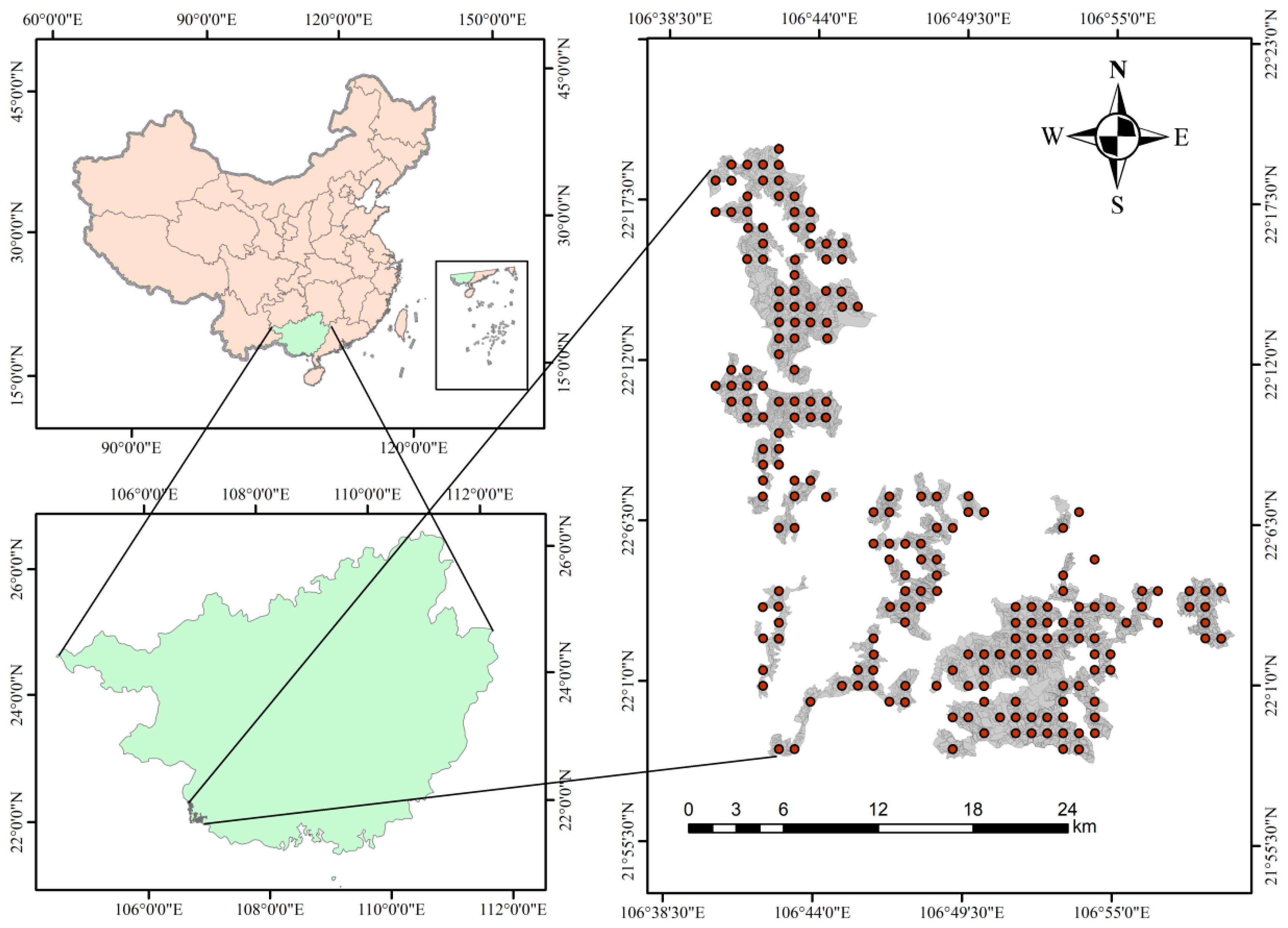
2.1. Study Sites

The study area was located within the Tropical Forest Research Center in Pingxiang City (21°57′ N to 22°16′ N, 106°41′ E to 109°59′ E), in the southwest of Guangxi Zhuang Autonomous Region in southern China (Figure 1). This region experiences the south Asian tropical monsoon climate, with an annual average air temperature of 20.5–21.7 °C. The average annual sunshine received is 1614 h, and the annual rainfall varies from 1062 to 1772 mm. The research area’s elevation spans from 250 to 800 m above sea level. Based on the Chinese soil classification system, the dominant soil type was red soil, which has developed from granite. According to the USDA (United States Department of Agriculture) Soil Taxonomy, this soil is equivalent to oxisols [24,25]. Pinus massoniana and Cunninghamia lanceolata are the most prevalent species, and mixed broad-leaved woods constitute the main form of vegetation [26].

2.2. Soil Sampling

Soil samples were collected in October 2020 during the low-rainfall season. Given the size of the study area and the homogeneity required for sampling, soil samples were collected at intersections on a 1 × 1 km grid, totaling 238 samples (Figure 1). Soil samples were taken at between 0 and 20 cm below the surface. Three subsamples in total were gathered at each of the 238 sample locations and pooled to create a single sample for each site. The subsamples were collected along an arc (radius of 6.51 m) located 8.49 m from the center of the site; subsamples were collected radially at the 0°, 120°, and 240° directions. Undisturbed soil cores were collected using a 100 cm³ or 200 cm³ cutting ring (referring to cylindrical metal cores). Forest soil water-physical properties (SM, SBD, CWHC, NCP, CP, and TP) were analyzed and determined according to the cutting ring method outlined in the forestry industry standard (LY/T 1215-1999) [27]. The distribution of sampling sites was visualized using ArcGIS 10.4.

2.3. Soil Measurements

Before sampling, the mass of the cutting ring (m₀) was accurately recorded. Once the sampling site was selected, the soil profile was excavated and a soil sample was taken using the cutting ring, ensuring that the soil structure within the ring knife was not damaged. The sample was then taken back to the laboratory to determine the weight of the soil core (m₁). The ring cutter with the fresh soil sample was placed in a plastic container with an appropriate amount of water added to ensure that the water level covered the upper edge of the ring cutter, and it soaked in a room-temperature environment for 12 h, at which point the total mass (m₂) was accurately recorded. Next, the soil samples were placed on dry sand to dry for 2 h, and their mass (m₃) was then recorded. Finally, the soil samples were placed in an oven and dried at 105 °C to determine the mass of the dried soil (m). The relevant formulas are given in Equations (1)–(6).

$$SM={\displaystyle \frac{m_1-m}{m}}\times 100$$

(1)

$$SBD={\displaystyle \frac{m}{V}}$$

(2)

$$CWHC={\displaystyle \frac{m_3-m_0-m}{m}}\times 100$$

(3)

$$NCP=\left({\displaystyle \frac{m_2-m_0-m}{m}}\times 100-CWHC\right)\times SBD$$

(4)

$$CP=CWHC\times SBD$$

(5)

$$TP=NCP+CP$$

(6)

where SM is the soil moisture (%); SBD is the soil bulk density (g/cm³); V is the volume of the cutting ring (cm³); CWHC is the capillary water-holding capacity (%); NCP is the non-capillary porosity (%); CP is the capillary porosity (%); and TP is the total porosity (%).

2.4. Statistical Methods

The associations between the variables were evaluated using Pearson correlation coefficients. All statistical analyses were performed in R 4.0.2. The implementation of the semivariance function, optimal run variance model, and ordinary kriging (OK) interpolations were carried out in R 3.5.1.

While geostatistical data could in principle be collected anywhere, local variations in topography and vegetation cover often make it difficult to directly measure soil water-physical properties at representative field sites. Therefore, variogram modeling was conducted based on spatial correlations among soil water-physical properties. Variograms are often used for spatial prediction (interpolation) or simulation of observed processes based on point observations. A semivariogram describing the spatial dependence of a random variable γ(h) over a given distance was estimated using Equation (7) [28].

$$\gamma \left(h\right)={\displaystyle \frac{1}{2N\left(h\right)}}{\displaystyle \sum }_{i=1}^{N\left(h\right)}{\left[z\left(x_i\right)-z\left(x_{i+h}\right)\right]}^2$$

(7)

where z(x_i) and z(x_i+h) denote the z-values at the locations $x_i$ and $x_{i+h}$, respectively; h is the lag; and N(h) is the number of pairs of sample points separated by h.

Most practical studies to date have used exponential, gaussian, linear and spherical models [29,30,31,32]. The models used in this study to estimate each semivariogram are given in Equations (8)–(11).

Exponential model:

$$\gamma \left(h\right)=\left\{\begin{array}{cc}\hfill C_0+\left[1-e^{\left(-{\displaystyle \frac{h}{a}}\right)}\right],& h\le a\hfill \\ \hfill C_0+C,& h>a\hfill \end{array}\right.$$

(8)

Spherical model:

$$\gamma \left(h\right)=\left\{\begin{array}{cc}\hfill C_0+C\left[{\displaystyle \frac{3}{2}}\left({\displaystyle \frac{h}{a}}\right)-{\displaystyle \frac{1}{2}}{\left({\displaystyle \frac{h}{a}}\right)}^3\right],& h\le a\hfill \\ \hfill C_0+C,& h>a\hfill \end{array}\right.$$

(9)

Linear model:

$$\gamma \left(h\right)=\left\{\begin{array}{cc}\hfill C_0+h\tan \theta ,& h\le a\hfill \\ \hfill C_0+C,& h>a\hfill \end{array}\right.$$

(10)

Gaussian model:

$$\gamma \left(h\right)=\left\{\begin{array}{cc}\hfill C_0+C\left[1-e^{-{\left({\displaystyle \frac{h}{a}}\right)}^2}\right],& h\le a\hfill \\ \hfill C_0+C,& h>a\hfill \end{array}\right.$$

(11)

where C₀ is the nugget variance; C is the structural variance; (C₀ + C) is the sill value of the semivariogram; and a is the range of spatial correlation [33,34].

In this study, the semivariograms for soil water-physical properties were characterized using exponential, linear, spherical, and gaussian models. The semivariograms were utilized to quantify spatial dependence and subsequently derive the essential parameters for interpolating target soil variables. These parameters (e.g., C₀, C, a, C₀ + C, and C₀/(C₀ + C)) described variation in different soil water-physical properties. The variogram models were fit using weighted least squares [35]. The variogram model deemed most appropriate for fit was the one with the highest coefficient of determination (R²) and the lowest residual sum of squares (RSS) [36]. For the purpose of analyzing spatial structure and obtaining interpolation input parameters, the best fit models were used [37]. The best linear unbiased estimate at sites where unobserved locations were available was determined using semivariograms. The term for this methodology referred to “kriging”, and kriged estimates of a given variable at point x₀ were calculated using Equation (12) [29]:

$$Z^{*}\left(x_0\right)={\displaystyle \sum }_{i=1}^n{w}_{i}Z\left(x_i\right)$$

(12)

where n is the number of sites at which measurements were taken; Z(x_i) is a measurement from the location x₀ used to estimate Z*(x₀); Z*(x₀) is the kriging estimate for location x₀; and w_i is the weight related to the distance between x₀ and x_i.

2.5. Model Validation

Cross-validation is a statistical approach for model validation that assesses the generalizability of results to an independent dataset. Here, the leave-one-out cross-validation method [38,39] was employed to evaluate prediction accuracy for each soil water-physical property. Statistical indices such as the absolute mean error (AME), mean error (ME), root mean square error (RMSE) [17], and R² [40] may reflect interpolation accuracy. These indices were calculated using Equations (13)–(16):

$$AME={\displaystyle \frac{1}{n}}{\displaystyle \sum }_{i=1}^n|\left(P_i-M_i\right)|$$

(13)

$$ME={\displaystyle \frac{1}{n}}{\displaystyle \sum }_{i=1}^n\left(P_i-M_i\right)$$

(14)

$$RMSE=\sqrt{{\displaystyle \frac{1}{n}}{\displaystyle \sum }_{i=1}^n{\left(P_i-M_i\right)}^2}$$

(15)

$$R^2=1-{\displaystyle \frac{{{\displaystyle \sum }}_{i=1}^n{\left(P_i-M_i\right)}^2}{{{\displaystyle \sum }}_{i=1}^n{\left(M_i-\overline{M}\right)}^2}}$$

(16)

where Pi, Mi, $\overline{M}$, and n are the predicted values, measured values, mean values of the measured data, and number of measured values, respectively.

3. Results and Discussion

3.1. Statistical Analysis of Soil Water-Physical Properties

Table 1. Statistical description of soil water-physical characteristics in the ECTF.

Physical Property	Mean	Min	Max	Med	SD	CV (%)	Skewness	Kurtosis	p-Value of S–W Test
SM (%)	31.07	10.48	64.65	30.32	10.15	0.33	0.39	−0.02	0.0817
SBD (g/cm3)	1.14	0.68	1.58	1.14	0.18	0.16	−0.16	−0.33	0.5932
CWHC (%)	43.62	20.30	102.30	42.30	13.64	0.31	1.10	2.15	<0.0001
NCP (%)	7.71	1.04	29.11	6.26	5.28	0.69	1.36	1.85	<0.0001
CP (%)	47.37	25.39	69.34	47.61	8.42	0.18	0.08	−0.39	0.7096
TP (%)	55.07	35.15	79.81	55.17	8.12	0.15	0.01	0.17	0.2800

Min: minimum; Max: maximum; Med: median; SD: standard deviation; CV: coefficient of variance; S–W test: Shapiro–Wilk test; SM: soil moisture; SBD: soil bulk density; CWHC: capillary water-holding capacity; NCP: non-capillary porosity; CP: capillary porosity; TP: total porosity.

shows the descriptive data for the soil’s water-physical characteristics. Soil water-physical properties varied widely and significantly among sampling sites within the study area. The maximum value of NCP was 27.99 times the minimum value, showing the wide range of values. The ratios of the maximum-to-minimum values for SM, CWHC, CP, SBD, and TP measured 6.17, 5.04, 2.73, 2.32, and 2.27, respectively. The coefficient of variation (CV) was calculated to quantify the variation in each soil property [41], representing a measure of the overall variation or heterogeneity in regional variables [42]. A CV of below 10% indicates little variability, while a CV ranging from 10% to 100% suggests moderate variability and a CV exceeding 100% signifies high variability [43]. Among the six soil water-physical properties, the CV ranged from 0.15 to 0.69, with the CV for NCP was much larger than that of the other soil water-physical properties. Variability (as assessed by the CV) increased from the TP to SBD, CP, CWHC, SM, and NCP; all soil water-physical properties showed moderate variability. The results of the Shapiro–Wilk test indicated that none of the properties showed a normal distribution except for SM, CP, SBD and TP among the soil water-physical properties. Therefore, CWHC and NCP were subjected to a logarithmic transformation prior to analysis in order to achieve a more normalized probability distribution.

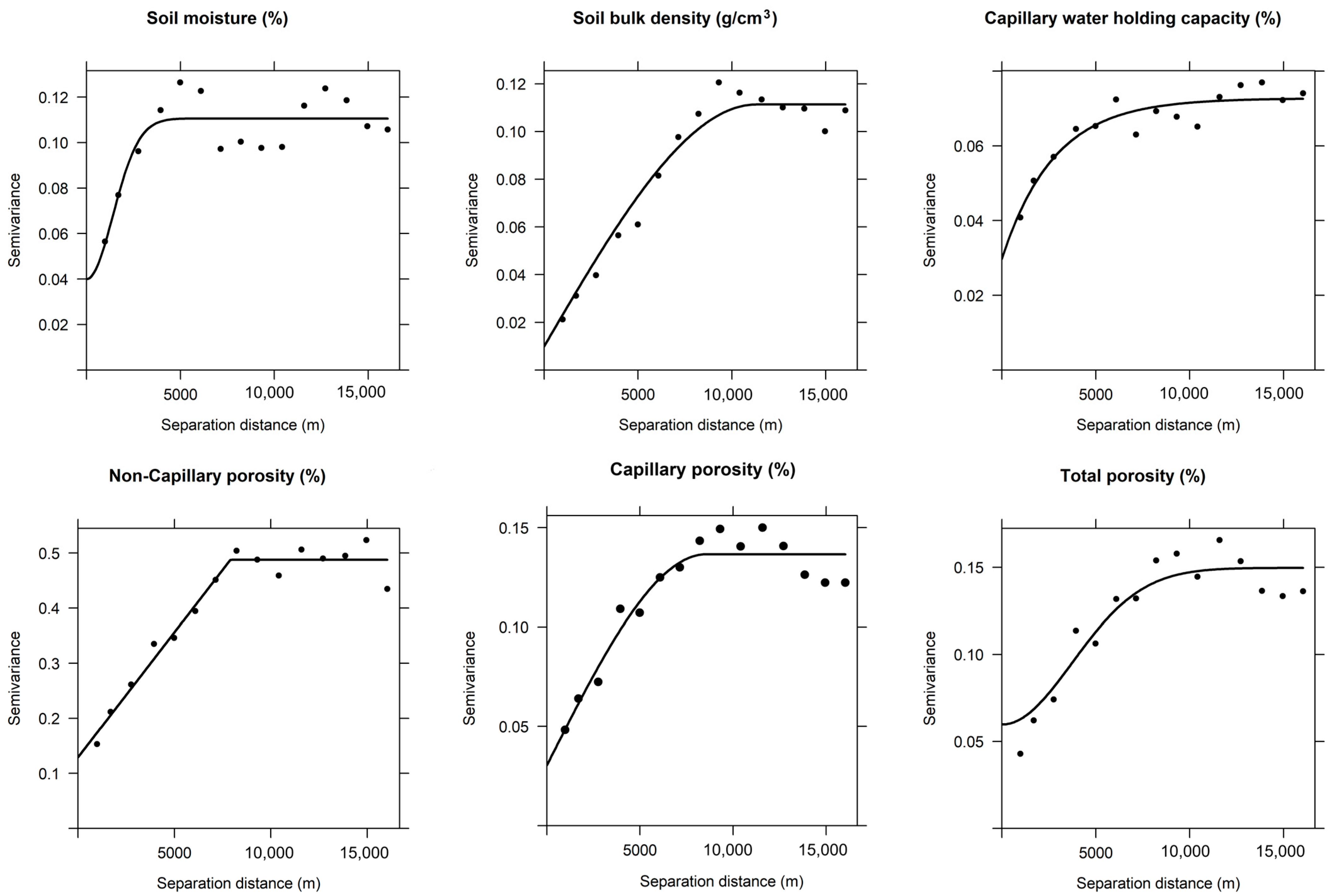
3.2. Spatial Variation Analysis for Soil Water-Physical Properties

Best-fit model parameters and several spatial structure indices are provided in

Table 2. Summary of best-fit semivariogram models for soil properties.

Physical Property	Model	Nugget (C0)	Sill (C0 + C)	Nugget/Sill C0/C0 + C	Range (A0, m)	R2	Residuals
SM (%)	Gau	0.04	0.11	0.36	3,419	0.723	0.00136
SBD (g/cm3)	Sph	0.01	0.11	0.09	11284	0.961	0.00003
CWHC (%)	Exp	0.03	0.07	0.41	8,340	0.880	0.00017
NCP (%)	Lin	0.13	0.48	0.26	7901	0.963	0.01764
CP (%)	Sph	0.03	0.14	0.22	8859	0.921	0.00127
TP (%)	Gau	0.02	0.09	0.22	14156	0.956	0.00035

Gau: Gaussian model; Exp: exponential model; Lin: linear model; Sph: spherical model; R²: coefficient of determination; SM: soil moisture; SBD: soil bulk density; CWHC: capillary water-holding capacity; NCP: non-capillary porosity; CP: capillary porosity; TP: total porosity.

. Across the soil water-physical properties, the nugget (C₀) value ranged from 0.01 to 0.13. This indicates that at the spatial scale of the study, some spatial variation was caused by sampling errors and random errors due to human interference. The nugget values were all relatively low, indicating that the sampling density used adequately captured the spatial structure of each soil physical property in the study area [44].

While the CV was used to determine the degree of variability in soil water-physical characteristics, it does not reveal the geographical distribution of each variable or the scale at which spatial heterogeneity occurred. The variable range (A₀) is the distance from the semivariance to the sill value. The presence of a sampling distance greater than A₀ indicates that observed values are mutually independent, and the data exhibit no spatial autocorrelation [45]. The variable range for the soil water-physical properties measured from 3419 m to 14,156 m (Table 2). The variable range was greatest for TP (14,156 m) and smallest for SM (3419 m). In all cases, the variable range was greater than the sampling distance (1000 m), so spatial interpolation could be effectively carried out. In a study of the spatial heterogeneity of soil water-physical properties in farmlands [46], with a mean sampling distance of 79.4 m, the variable range measured 106 m for surface SBD and the spatial dependence was 29%. Compared to this study, the sampling scale and minimum sampling distance were both reduced (i.e., less than 1000 m) in the farmland study, and the variable range was thus also smaller. Scale effects may moderate observed spatial heterogeneity; therefore, studies spanning multiple scales may better capture spatial variability in soil water-physical properties and more accurately describe their spatial distributions [47]. Due to scale effects, the spatial heterogeneity observed for soil water-physical properties may be quite different across sampling scales. At the same time, quantifying scale effects may improve the accuracy of soil investigations, with different sampling scales being useful for different research purposes. Given the variable range of 3000+ m for soil water-physical properties, future studies of woodland soils should select a sampling scale accordingly.

According to the research by Cambardella et al. [48], a nugget-to-sill ratio (C₀/(C₀ + C)) was used for spatial dependence assessment. The presence of strong spatial dependence is indicated by a ratio below 25%, while a ratio from 25 to 75% indicates moderate dependence; when the ratio approaches 1, spatial dependence is low, suggesting a high level of measurement error [49]. Differences in the degree of spatial dependence are caused by both intrinsic and extrinsic factors [45]. In general, substantial geographic dependency in soil characteristics is associated to intrinsic structural elements such as soil mineralogy, parent materials, and texture, whereas moderate spatial dependence is related to randomized extrinsic factors such as fertilization, plowing, and other soil management activities [50]. In this investigation, SBD, CP, and TP exhibited considerable spatial dependency, with a C₀/(C₀ + C) value of less than 25%. Similar results were also seen by Naitam, et al. [51], who attributed the strong spatial autocorrelation observed to underlying patterns in soil type, texture, and parent material, as well as topography and other structural factors. In contrast, in Gülser, et al. [52], the moderate autocorrelation observed for SBD was likely shaped by regular plowing, as an extrinsic factor known to reduce spatial dependence.

As seen in the semivariograms (Figure 2), CWHC, SM, and NCP all exhibited moderate spatial dependency, with C₀/(C₀ + C) values ranging from 25 to 75%. Moderate spatial dependency can be influenced by a mix of internal and extrinsic variables, such as soil formation processes and fertilizer application and tillage [48,53]. Other studies have described moderate spatial dependence of soil water-physical properties (e.g., soil texture, SBD, and SM) [54,55,56]. In this study, moderate to strong spatial dependence was found for soil water-physical properties, in contrast to the findings of other studies [11,51,57].

In addition, the coefficient of determination (R²) measured close to one (range: 0.723–0.963) for all soil water-physical properties, indicating that high precision was achieved by the theoretical models. Similar results have also been reported for many other studies [45]. For example, Ghorbani, et al. [58] obtained that among the semivariate models, exponential, Gaussian, linear and spherical models were described as the best fit (R² of 0.97–0.99) for the water-physical properties of soil water, similar to the results of this study.

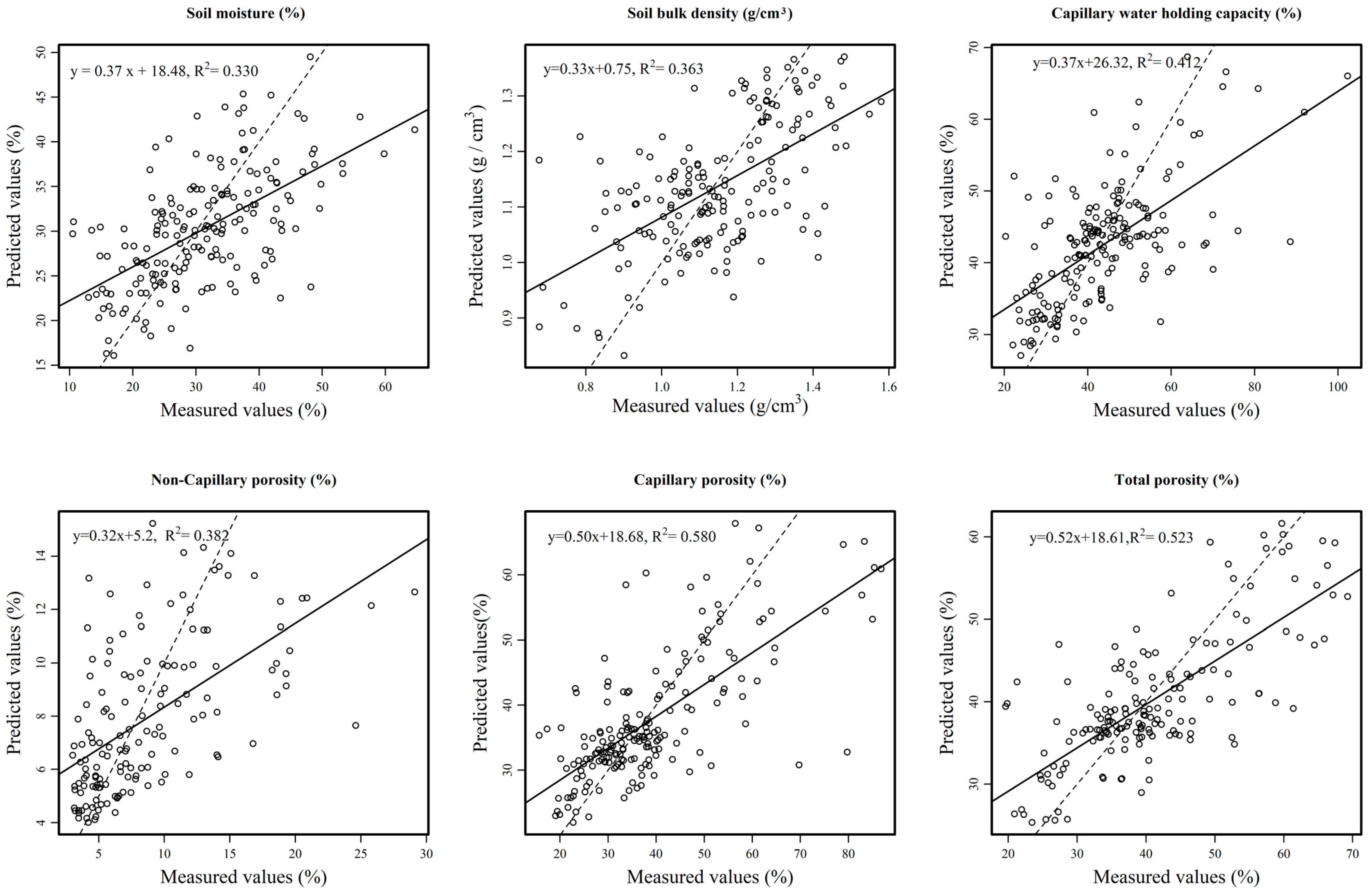
3.3. Ordinary Kriging Model Validation

Table 3. Semivariogram model cross-validation for soil water-physical properties in the ECTF forest.

Physical Property	AME	ME	RMSE
SM (%)	0.2171	0.0043	0.2833
SBD (g/cm3)	0.0940	−0.0006	0.1295
CWHC (%)	0.1701	0.0009	0.2303
NCP (%)	0.2807	0.0010	0.3851
CP (%)	0.1786	0.0011	0.2414
TP (%)	0.1431	0.0009	0.1903

AME: absolute mean error; ME: mean error; RMSE: root mean square error; SM: soil moisture; SBD: soil bulk density; CWHC: capillary water-holding capacity; NCP: non-capillary porosity; CP: capillary porosity; TP: total porosity.

displays the assessment indices derived from cross-validation of regional distribution maps of soil water-physical parameters (Figure 3). A mean error (ME) value close to zero implies that the overall estimation bias is minimal. A root mean square error (RMSE) value close to zero indicates high interpolation precision [59]. The absolute mean error (AME) was constructed to assess the difference between observed and interpolated values [60]. For all OK models, the ME was close to zero, suggesting a lack of bias in interpolating soil water-physical properties. For SM, CP, NCP, CWHC, TP, and SBD, the ME measured 0.0043, 0.0011, 0.0010, 0.0009, 0.0009, and −0.0006, respectively. The interpolation of soil water-physical characteristics produced RMSE values ranging from 0.1295 to 0.3851. Low ME and RMSE values indicated a good match between observed and projected soil water-physical characteristics.

Figure 3 shows the connection between measured and predicted outcomes for all sample sites. Points near the 1:1 reference line illustrate cases where the predicted values were extremely close to the measured values, representing highly precise predictions. In theory, the best projections should be based on actual measured data. However, due to smoothing effects during spatial interpolation, the regression slope (for measured versus anticipated values) was always less than one [45]. The slope measured 0.52 for TP, 0.50 for CP, 0.37 for CWHC, 0.37 for SM, 0.33 for SBD and 0.32 for NCP. The slope for TP was higher than that of other soil water-physical properties, indicating higher precision for TP predictions. For all soil water-physical properties, the cross-validation R² ranged from 0.330 to 0.580, suggesting that spatial prediction using semivariogram parameters was a reasonable approach to describing spatial variation. The range of R² values was similar to that reported by other studies (e.g., 0.332–0.596; Golden, et al. [61]).

As seen from the observed-predicted value regressions and model cross-validation results, OK represented a good approach for accurately interpolating spatial variability in soil water-physical properties. The selection of appropriate methods to study soil variation can effectively improve data collection and provide a solid scientific basis for precision soil management.

3.4. Pearson Correlation Analysis for Soil Water-Physical Properties

Pearson correlation coefficients represent a measure of the linear correlation between two variables. Correlation coefficients vary between one and minus one, with a value of one representing a perfect positive correlation, zero a lack of correlation, and minus one a perfect negative correlation [45]. Pearson correlation coefficients for the soil water-physical properties are shown in

Table 4. Correlation matrix for the soil water-physical properties.

Physical Property	SM	SBD	CWHC	NCP	CP	TP
SM	1
SBD	−0.660 **	1
CWHC	0.809 **	−0.833 **	1
NCP	−0.004	−0.320 **	−0.071	1
CP	0.785 **	−0.499 **	0.851 **	−0.368 **	1
TP	0.810 **	−0.725 **	0.835 **	0.269 **	0.796 **	1

** p < 0.01; SM: soil moisture; SBD: soil bulk density; CWHC: capillary water-holding capacity; NCP: non-capillary porosity; CP: capillary porosity; TP: total porosity.

. SM was significantly and positively correlated with TP (0.810), CWHC (0.809), and CP (0.785). However, SM was significantly and negatively correlated with SBD (−0.660). This indicates that the greater the soil’s porosity and capillary activity, the stronger its ability to retain moisture. SBD was negatively correlated with CWHC (−0.833), TP (−0.725), CP (−0.499), and NCP (−0.320). This suggests that decreases in SBD in forested areas are beneficial to soil permeability and water retention. Variation in SBD may result from differences in soil organic matter content and texture, as well as in soil management practices [62]. In other words, due to the high levels of disturbance associated with human activities in cultivated areas (e.g., fertilization and tilling), soil physical and structural properties may be greatly altered, as may be the relationships among soil water-physical properties. Additionally, climate variables (precipitation and temperature) [63,64] and other factors (other soil properties, topography, etc.) [65,66] may also shape the relationships among soil water-physical properties.

3.5. Spatial Distribution Map

Figure 4 shows thematic maps for the soil water-physical properties produced via OK. The spatial distributions of SM and CWHC were broadly consistent. Predicted values ranged from 15.82% to 51.00% for SM, from 0.74 g/cm³ to 1.47 g/cm³ for SBD, from 25.80% to 78.10% for CWHC, from 0% to 30% for NCP, from 25.00% to 70.00% for CP, and from 25.03% to 63.11% for TP. The greatest spatial variation was observed for CWHC, followed by CP, TP, SM, NCP, and SBD.

The spatial distribution patterns of SM and CWHC were more similar, both showing an increasing trend from the southeast corner to the northwest corner. The lowest values of both occurred in the southeastern corner of the study area, where pure Masson pine forests were dominant. This spatial pattern may have been shaped by the following two effects. First, Masson pine is a fast-growing tree species with a short rotation harvest period and high consumption of nutrients and water. Second, coniferous tree litter contains relatively more oils and is resistant to both absorbing and storing water. In contrast, the highest values of SM and CWHC occurred in the northwest, where mixed-species broadleaved forests were dominant. High SM levels may have been due to the canopy density and strong shading effects of coniferous and broadleaved mixed forests in the northwest, as the SM content can be enhanced by reducing surface evaporation and soil erosion due to rain. When comparing forest types, mixed stands typically absorb less water from the soil than pure stands [67]. In conclusion, surface SM levels in mixed broadleaved forests were higher than those of single-species forests.

SBD exhibited the opposite spatial pattern to SM, being highest in the southeast and lowest in the northwest. In the northwestern parts of the study area, where there were more coniferous trees, SBD was significantly lower. One possible explanation is that pure Masson pine forests (in the south) grew rapidly, absorbing large amounts of water and nutrients and increasing soil hardness as a result. Due to reductions in litter volume and slower decomposition, as well as decreased shading of the ground, the soil was more frequently exposed to the sun, resulting in hardening and increased bulk density. Here, mixed forests showed lower SBD and higher SM. To reduce bulk density in the southern part of the study area, periodic perforation and ventilation of the topsoil around trees is recommended. Planting shrubs and herbaceous species within 2 m of tree trunks is also recommended to reduce the trampling frequency [10].

In the eastern part of the study area, the water-physical characteristics of the soil, with the exception of the SBD indicator, show low levels. This condition is closely related to the relatively low altitude of the region and the greater influence of human activities [68]. Especially in the eastern zone, dominated by the cultivation of Fir and Horsetail pine, the soil is more sensitive to trampling and compaction due to the monoculture hierarchy of the tree species and the shallow and predominantly topsoil root system [7]. As a result, the SM, CWHC, NCP, CP, and TP of the soil were generally lower in the east versus the rest of the study [69] area, and SBD is generally higher than in other regions. In other studies, soil TP and CP are often positively correlated with root density, which could be used to predict root density [10,70]. Based on this, soil porosity can be effectively enhanced by planting tree species with high root density and wide distribution, such as Camphora officinarum, Zelkova serrata, Koelreuteria paniculata, and Metasequoia glyptostroboides [7,10]. Similarly, we can improve the water-physical properties of the soil by planting Castanopsis lamontii and Castanopsis sclerophylla in the masson pine pure forest of the eastern study area [69]. Based on our study of thematic maps of soil water-physical properties in southern subtropical forests in China, we are able to recognize the initial signs of soil degradation in time and implement appropriate restoration strategies accordingly. We should adopt adaptive management strategies to enhance active human intervention, reduce human-induced disturbance, and improve the water-physical properties of soils to improve forest productivity.

4. Conclusions

This study used OK modeling to characterize spatial variation in soil water-physical properties. Among the four OK models assayed, an exponential model was determined to be the most suitable fit for CWHC, while a Gaussian model was the best fit for SM and TP. For NCP, a linear model was identified as the optimal fit based on the experimental semivariogram analysis. For SBD and CP, a spherical model emerged as the most appropriate fit according to the experimental semivariogram. Soil property semivariograms revealed that, with the exception of SBD, CP and TP, all other soil water-physical properties were moderately spatially dependent. Geographical maps of the soil water-physical properties identified high values for CWHC and SM in the northwest, while the southern part of the study area had the highest SBD, CP, NCP, and TP. With the exception of SBD, the values of other soil physical property indicators in the eastern part of the study area were lower than the corresponding values in the other directions. Many soil water-physical properties were significantly correlated and strongly interdependent. Cross-validation of OK-derived maps revealed that semivariogram parameters improved predictions of soil water-physical properties in unsampled locations. The interpolated maps created in this study could serve as a useful tool for pinpointing regions of degradation in the study area and creating precise land management plans.

References

1. Phogat, V.K.; Tomar, V.S.; Dahiya, R. Soil Physical Properties. 2015, Chapter 6, pp. 135–171. Available online: https://www.researchgate.net/publication/297737054_Soil_Physical_Properties (accessed on 28 July 2024).
2. Ghestem, M.; Sidle, R.C.; Stokes, A. The Influence of Plant Root Systems on Subsurface Flow: Implications for Slope Stability. BioScience 2011, 61, 869–879. [Google Scholar] [CrossRef]
3. Moran, M.S.; Peters-Lidard, C.D.; Watts, J.M.; Mcelroy, S. Estimating soil moisture at the watershed scale with satellite-based radar and land surface models. Can. J. Remote Sens. 2004, 30, 805–826. [Google Scholar] [CrossRef]
4. Verstraeten, W.W.; Veroustraete, F.; Wagner, W.; Roey, V.; Heyns, W.; Verbeiren, S.; Sande, C.J.V.D.; Feyen, J. Impact Assessment of Remotely Sensed Soil Moisture on Ecosystem Carbon Fluxes across Europe. In Proceedings of the International Workshop on Uncertainty in Greenhouse Gas Inventories, Laxenburg, Austria, 27–28 September 2007; Available online: https://api.semanticscholar.org/CorpusID:133238608 (accessed on 28 July 2024).
5. Zheng, F.L. Effect of Vegetation Changes on Soil Erosion on the Loess Plateau. Pedosphere 2006, 16, 420–427. [Google Scholar] [CrossRef]
6. Zhu, Y.; Irmak, S.; Jhala, A.J.; Vuran, M.C.; Diotto, A.V. Time-domain and Frequency-domain Reflectometry Type Soil Moisture Sensor Performance and Soil Temperature Effects in Fine- and Coarse-textured Soils. Appl. Eng. Agric. 2019, 35, 117–134. [Google Scholar] [CrossRef]
7. Bartens, J.; Wiseman, P.E.; Smiley, E.T. Stability of landscape trees in engineered and conventional urban soil mixes. Urban For. Urban Green. 2010, 9, 333–338. [Google Scholar] [CrossRef]
8. Gao, R.; Shi, J.; Huang, R.; Wang, Z.; Luo, Y. Effects of pine wilt disease invasion on soil properties and Masson pine forest communities in the Three Gorges reservoir region, China. Ecol. Evol. 2015, 5, 1702–1716. [Google Scholar] [CrossRef] [PubMed]
9. Sasal, M.C.; Andriulo, A.E.; Taboada, M.A. Soil porosity characteristics and water movement under zero tillage in silty soils in Argentinian Pampas. Soil Tillage Res. 2006, 87, 9–18. [Google Scholar] [CrossRef]
10. Yu, B.; Xie, C.; Cai, S.; Chen, Y.; Lv, Y.; Mo, Z.; Liu, T.; Yang, Z. Effects of Tree Root Density on Soil Total Porosity and Non-Capillary Porosity Using a Ground-Penetrating Tree Radar Unit in Shanghai, China. Sustainability 2018, 10, 4640. [Google Scholar] [CrossRef]
11. Wang, Y.Q.; Shao, M.A. Spatial Variability of Soil Physical Properties in a Region of the Loess Plateau of PR China Subject to Wind and Water Erosion. Land Degrad. Dev. 2013, 24, 296–304. [Google Scholar] [CrossRef]
12. Legendre, P. Spatial Autocorrelation: Trouble or New Paradigm? Ecology 1993, 74, 1659–1673. [Google Scholar] [CrossRef]
13. Berndtsson, R.; Bahri, A.; Jinno, K. Spatial Dependence of Geochemical Elements in a Semiarid Agricultural Field: II. Geostatistical Properties. Soil Sci. Soc. Am. J. 1993, 57, 289–295. [Google Scholar] [CrossRef]
14. Brady, N.C. The nature and properties of soils. 10th ed. J. Range Manag. 1990, 5, 333. [Google Scholar]
15. da Luz, F.B.; Carvalho, M.L.; Castioni, G.A.F.; de Oliveira Bordonal, R.; Cooper, M.; Carvalho, J.L.N.; Cherubin, M.R. Soil structure changes induced by tillage and reduction of machinery traffic on sugarcane—A diversity of assessment scales. Soil Tillage Res. 2022, 223, 105469. [Google Scholar] [CrossRef]
16. Alwazzan, T.T.; Atti, A.S.J.I.C.S.E.; Science, E. Evaluation of Soil Quality and Health Indices in Relation to Soil Physical Properties of Fedak Farm in Holly Najaf Province. IOP Conf. Ser. Earth Environ. Sci. 2022, 1060, 012023. [Google Scholar] [CrossRef]
17. Reza, S.K.; Nayak, D.C.; Chattopadhyay, T.; Mukhopadhyay, S.; Srinivasan, R. Spatial distribution of soil physical properties of alluvial soils: A geostatistical approach. Arch. Agron. Soil Sci. 2015, 62, 151013100517007. [Google Scholar] [CrossRef]
18. Mueller, T.G.; Pierce, F.J. Soil Carbon Maps: Enhancing Spatial Estimates with Simple Terrain Attributes at Multiple Scales. Soil Sci. Soc. Am. J. 2003, 67, 258–267. [Google Scholar] [CrossRef]
19. Bostan, P. Assessing variations in climate extremes over Euphrates Basin, Turkey. Theor. Appl. Climatol. 2020, 141, 1461–1473. [Google Scholar] [CrossRef]
20. Shahbeik, S.; Afzal, P.; Moarefvand…, P. Comparison between ordinary kriging (OK) and inverse distance weighted (IDW) based on estimation error. Case study: Dardevey iron ore deposit, NE Iran. Arab. J. Geosci. 2014, 7, 3693–3704. [Google Scholar] [CrossRef]
21. Ouabo, R.E.; Sangodoyin, A.Y.; Ogundiran, M.B. Assessment of Ordinary Kriging and Inverse Distance Weighting Methods for Modeling Chromium and Cadmium Soil Pollution in E-Waste Sites in Douala, Cameroon. J. Health Pollut. 2020, 10, 200605. [Google Scholar] [CrossRef]
22. Silatsa, F.B.T.; Yemefack, M.; Tabi, F.O.; Heuvelink, G.B.M.; Leenaars, J.G.B. Assessing countrywide soil organic carbon stock using hybrid machine learning modelling and legacy soil data in Cameroon. Geoderma 2020, 367, 114260. [Google Scholar] [CrossRef]
23. Yang, H.; Huang, T.; Li, Y.; Liu, W.; Fu, J.; Huang, B.; Yang, Q. Spatial heterogeneity and influence mechanisms on soil respiration in an old-growth tropical montane rainforest with complex terrain. Front. Ecol. Evol. 2023, 10, 1107421. [Google Scholar] [CrossRef]
24. Huang, X.; Liu, S.; Wang, H.; Hu, Z.; Li, Z.; You, Y. Changes of soil microbial biomass carbon and community composition through mixing nitrogen-fixing species with Eucalyptus urophylla in subtropical China. Soil Biol. Biochem. 2014, 73, 42–48. [Google Scholar] [CrossRef]
25. Wang, H.; Liu, S.; Wang, J.; Shi, Z.; Lu, L.; Guo, W.; Jia, H.; Cai, D. Dynamics and speciation of organic carbon during decomposition of leaf litter and fine roots in four subtropical plantations of China. For. Ecol. Manag. 2013, 300, 43–52. [Google Scholar] [CrossRef]
26. Meng, J.; Lu, Y.; Zeng, J. Transformation of a Degraded Pinus massoniana Plantation into a Mixed-Species Irregular Forest: Impacts on Stand Structure and Growth in Southern China. Forests 2014, 5, 3199–3221. [Google Scholar] [CrossRef]
27. LY/T1215-1999; Determination of Forest Soil Water-Physical Properties. Standards Press of China: Beijing, China, 1999; pp. 21–24.
28. Robertson, G.P. Geostatistics in Ecology: Interpolating With Known Variance. Ecology 1987, 68, 744–748. [Google Scholar] [CrossRef]
29. Gupta, N.; Rudra, R.P.; Parkin, G.; Parkin, R.P. Analysis of spatial variability of hydraulic conductivity at field scale. Can. Biosyst. Eng. 2006, 48, 155–161. Available online: https://www.researchgate.net/publication/229047388 (accessed on 28 July 2024).
30. Betzek, N.M.; Souza, E.G.D.; Bazzi, C.L.; Schenatto, K.; Gavioli, A.; Magalhães, P.S.G. Computational routines for the automatic selection of the best parameters used by interpolation methods to create thematic maps. Comput. Electron. Agric. 2019, 157, 49–62. [Google Scholar] [CrossRef]
31. Zandi, S.; Ghobakhlou, A.; Sallis, P. Evaluation of Spatial Interpolation Techniques for Mapping Soil pH; Modelling and Simulation Society of Australia and New Zealand: Perth, Australia, 2011; pp. 1153–1159. [Google Scholar] [CrossRef]
32. Gao, X.; Xiao, Y.; Deng, L.; Qiquan, L.I.; Wang, C.; Bing, L.I.; Deng, O.; Zeng, M. Spatial variability of soil total nitrogen, phosphorus and potassium in Renshou County of Sichuan Basin, China. J. Integr. Agric. 2019, 18, 279–289. [Google Scholar] [CrossRef]
33. Samra, J.S.; Singh, V.P.; Sharma, K.N.S. Analysis of spatial variability in sodic soils: 2. Point- and block-kriging. Soil Sci. 1988, 145, 250–256. [Google Scholar] [CrossRef]
34. Bivand, R.S.; Pebesma, E.; Gómez-Rubio, V. Chapter 8: Interpolation and Geostatistics. In Applied Spatial Data Analysis with R; Springer: New York, NY, USA, 2013; Volume 10, pp. 232–260. [Google Scholar] [CrossRef]
35. Cressie, N. Fitting variogram models by weighted least squares. J. Int. Assoc. Math. Geol. 1985, 17, 563–586. [Google Scholar] [CrossRef]
36. Liu, Z.-P.; Shao, M.-A.; Wang, Y.-Q. Spatial patterns of soil total nitrogen and soil total phosphorus across the entire Loess Plateau region of China. Geoderma 2013, 197–198, 67–78. [Google Scholar] [CrossRef]
37. Guan, F.; Xia, M.; Tang, X.; Fan, S. Spatial variability of soil nitrogen, phosphorus and potassium contents in Moso bamboo forests in Yong’an City, China. CATENA 2017, 150, 161–172. [Google Scholar] [CrossRef]
38. Kim, M.; Kim, H.-S.; Chung, C.-K. A Three-Dimensional Geotechnical Spatial Modeling Method for Borehole Dataset Using Optimization of Geostatistical Approaches. KSCE J. Civ. Eng. 2020, 24, 778–793. [Google Scholar] [CrossRef]
39. Gyasi-Agyei, Y. Identification of the Optimum Rain Gauge Network Density for Hydrological Modelling Based on Radar Rainfall Analysis. Water 2020, 12, 1906. [Google Scholar] [CrossRef]
40. Liu, Z.P.; Shao, M.A.; Wang, Y.Q. Large-scale spatial interpolation of soil pH across the Loess Plateau, China. Environ. Earth Sci. 2013, 69, 2731–2741. [Google Scholar] [CrossRef]
41. Wang, Y.; Li, Y.; Xiao, D. Catchment scale spatial variability of soil salt content in agricultural oasis, Northwest China. Environ. Geol. 2008, 56, 439–446. [Google Scholar] [CrossRef]
42. Liu, Z.P.; Shao, M.A.; Wang, Y.Q. Large-scale spatial variability and distribution of soil organic carbon across the entire Loess Plateau, China. Soil Res. 2012, 50, 114–124. [Google Scholar] [CrossRef]
43. Fang, X.; Xue, Z.; Li, B.; An, S. Soil organic carbon distribution in relation to land use and its storage in a small watershed of the Loess Plateau, China. Catena 2012, 88, 6–13. [Google Scholar] [CrossRef]
44. Mcgrath, D.; Zhang, C.; Carton, O.T. Geostatistical analyses and hazard assessment on soil lead in Silvermines area, Ireland. Environ. Pollut. 2004, 127, 239–248. [Google Scholar] [CrossRef]
45. Yan, P.; Peng, H.; Yan, L.; Lin, K. Spatial Variability of Soil Physical Properties Based on GIS and Geo-Statistical Methods in the Red Beds of the Nanxiong Basin, China. Pol. J. Environ. Stud. 2019, 28, 2961–2972. [Google Scholar] [CrossRef]
46. Iqbal, J.; Thomasson, J.A.; Jenkins, J.N.; Owens, P.R.; Whisler, F.D. Spatial Variability Analysis of Soil Physical Properties of Alluvial Soils. Soil Sci. Soc. Am. J. 2005, 69, 1338–1350. [Google Scholar] [CrossRef]
47. Wentz, E.A. Modelling Scale in Geographical Information Science (review). Geogr. Anal. 2003, 35, 177–178. [Google Scholar] [CrossRef]
48. Cambardella, C.A.; Moorman, T.B.; Novak, J.M.; Parkin, T.B.; Konopka, A.E. Field-Scale Variability of Soil Properties in Central Iowa Soils. Soil Sci. Soc. Am. J. 1994, 58, 1501–1511. [Google Scholar] [CrossRef]
49. Robertson, G.P.; Klingensmith, K.M.; Klug, M.J.; Paul, E.A.; Crum, J.R.; Ellis, B.G. Soil Resources, Microbial Activity, and Primary Production across an Agricultural Ecosystem. Ecol. Appl. 1997, 7, 158–170. [Google Scholar] [CrossRef]
50. Zheng, H.; Wu, J.; Zhang, S. Study on the Spatial Variability of Farmland Soil Nutrient Based on the Kriging Interpolation. In Proceedings of the 2009 International Conference on Artificial Intelligence and Computational Intelligence, Shanghai, China, 7–8 November 2009; Volume 4, pp. 550–555. [Google Scholar] [CrossRef]
51. Naitam, R.; Kharche, V.; Kadu, P.; Mohrana, P.; Sharma, R. Field-scale spatial variability of physical properties of black soils of Purna Valley, India, using Geostatistical Approach. J. Soil Water Conserv. 2018, 17, 325–334. [Google Scholar] [CrossRef]
52. Gülser, C.; Ekberli, I.; Candemir, F. Spatial variability of soil physical properties in a cultivated field. Eur. J. Soil Sci. 2016, 5, 192–200. Available online: https://www.researchgate.net/publication/300071023 (accessed on 28 July 2024).
53. Reza, S.K.; Dutta, D.; Bandyopadhyay, S.; Singh, S.K. Spatial Variability Analysis of Soil Properties of Tinsukia District, Assam, India. Agric. Res. 2018, 8, 231–238. [Google Scholar] [CrossRef]
54. Safari, Y.; Esfandiarpour Boroujeni, I.; Kamali, A.; Salehi, M.H.; Bagheri Bodaghabadi, M. Mapping of the soil texture using geostatistical method (a case study of the Shahrekord plain, central Iran). Arab. J. Geosci. 2012, 6, 3331–3339. [Google Scholar] [CrossRef]
55. Jabro, J.D.; Stevens, B.W.; Evans, R.G. Spatial Relationships among Soil Physical Properties in a Grass-Alfalfa Hay Field. Soil Sci. 2006, 171, 719–727. [Google Scholar] [CrossRef]
56. Liu, C.L.; Wu, Y.Z.; Liu, Q.J. Effects of land use on spatial patterns of soil properties in a rocky mountain area of Northern China. Arab. J. Geosci. 2015, 8, 1181–1194. [Google Scholar] [CrossRef]
57. Duffera, M.; White, J.G.; Weisz, R. Spatial variability of Southeastern U.S. Coastal Plain soil physical properties: Implications for site-specific management. Geoderma 2007, 137, 327–339. [Google Scholar] [CrossRef]
58. Ghorbani, M.A.; Deo, R.C.; Kashani, M.H.; Shahabi, M.; Ghorbani, S. Artificial intelligence-based fast and efficient hybrid approach for spatial modelling of soil electrical conductivity. Soil Tillage Res. 2019, 186, 152–164. [Google Scholar] [CrossRef]
59. Qu, L.; Xiao, H.; Zheng, N.; Zhang, Z.; Xu, Y. Comparison of four methods for spatial interpolation of estimated atmospheric nitrogen deposition in South China. Environ. Sci. Pollut. Res. 2016, 24, 2578–2588. [Google Scholar] [CrossRef]
60. Riggers, C.; Poeplau, C.; Don, A.; Bamminger, C.; Dechow, R. Multi-model ensemble improved the prediction of trends in soil organic carbon stocks in German croplands. Geoderma 2019, 345, 17–30. [Google Scholar] [CrossRef]
61. Golden, N.; Zhang, C.; Potito, A.; Gibson, P.J.; Bargary, N.; Morrison, L. Use of ordinary cokriging with magnetic susceptibility for mapping lead concentrations in soils of an urban contaminated site. J. Soils Sediments 2019, 20, 1357–1370. [Google Scholar] [CrossRef]
62. Wolf, B. Sustainable Soils: The Place of Organic Matter in Sustaining Soils and Their Productivity; CRC Press: New York, NY, USA, 2003. [Google Scholar]
63. Bi, X.; Li, B.; Nan, B.; Fan, Y.; Fu, Q.; Zhang, X. Characteristics of soil organic carbon and total nitrogen under various grassland types along a transect in a mountain-basin system in Xinjiang, China. J. Arid. Land 2018, 10, 612–627. [Google Scholar] [CrossRef]
64. Li, Y.; Zeng, C.; Long, M. Variation of soil nutrients and bacterial community diversity of different land utilization types in Yangtze River Basin, Chongqing Municipality. PeerJ 2020, 8, e9386. [Google Scholar] [CrossRef] [PubMed]
65. Bogunovic, I.; Pereira, P.; Brevik, E.C. Spatial distribution of soil chemical properties in an organic farm in Croatia. Sci. Total Environ. 2017, 584–585, 535–545. [Google Scholar] [CrossRef]
66. Luo, M.; Guo, L.; Zhang, H.; Wang, S.; Liang, P. Characterization of Spatial Distribution of Soil Organic Carbon in China Based on Environmental Variables. Acta Pedol. Sin. 2020, 57, 48–59. [Google Scholar] [CrossRef]
67. Zhang, B.; Xu, Q.; Gao, D.; Jiang, C.; Liu, F.; Jiang, J.; Wang, T. Altered water uptake patterns of Populus deltoides in mixed riparian forest stands. Sci. Total Environ. 2020, 706, 135956. [Google Scholar] [CrossRef]
68. Toivio, J.; Helmisaari, H.-S.; Palviainen, M.; Lindeman, H.; Ala-Ilomäki, J.; Sirén, M.; Uusitalo, J. Impacts of timber forwarding on physical properties of forest soils in southern Finland. For. Ecol. Manag. 2017, 405, 22–30. [Google Scholar] [CrossRef]
69. Lin, D.; Fan, H.; Su, B.; Liu, C.; Jiang, Z. Effect of interplantation of broad-leaved trees in Pinus massoniana forest on physical and chemical properties of the soil. Acta Pedol. Sin. 2004, 41, 655–659. [Google Scholar]
70. Yusheng, Y.; Guangshui, C.; Zongming, H.; Amp, C.Y.; Jianfen, G. Production, distribution and nutrient return of fine roots in a mixed and a pure forest in subtropical China. Chin. J. Appl. Environ. Biol. 2002, 8, 223–233. Available online: https://api.semanticscholar.org/CorpusID:87895541 (accessed on 28 July 2024).
Figure 1. Distribution of the 238 sample plots within the study area and location of the study area within China.
Forests 15 01590 g001
Figure 2. Semivariograms with fitted models for each soil water-physical property.
Forests 15 01590 g002
Figure 3. Cross-validation of ordinary kriging interpolation of soil water-physical properties (the dashed line represents a 1:1 relationship).
Forests 15 01590 g003
Figure 4. Thematic maps of soil water-physical properties produced using OK models and interpolation.
Forests 15 01590 g004