Quantitative Evaluation of the Applicability of Classical Forest Ecosystem Carbon Cycle Models in China: A Case Study of the Biome-BGC Model

Abstract

The Biome-BGC model is a classic forest ecosystem carbon cycle model driven by remote sensing and plant trait data, and it has been widely applied in various regions of China over the years. However, does the Biome-BGC model have good applicability in all regions of China? This question implies that the rationality of some applications of the Biome-BGC model in China might be questionable. To quantitatively assess the overall spatial applicability of the Biome-BGC model in China’s vegetation ecosystems, this study selected ten representative forest and grassland ecosystem sites, all of which have publicly available carbon flux data. In this study, we first used the EFAST method to identify the sensitive ecophysiological parameters of the Biome-BGC model at these sites. Subsequently, we calibrated the optimal values of these sensitive parameters through a literature review and the PEST method and then used these to drive the Biome-BGC model to simulate the productivity (including GPP and NEP) of these ten forest and grassland ecosystems in China. Finally, we compared the simulation accuracy of the Biome-BGC model at these ten sites in detail and established the spatial pattern of the model’s applicability across China. The results show that the sensitive ecophysiological parameters of the Biome-BGC model vary with spatial distribution, plant functional types, and model output variables. After conducting parameter sensitivity analysis and optimization, the simulation accuracy of the Biome-BGC model can be significantly improved. Additionally, for forest ecosystems in China, the model’s simulation accuracy decreases from north to south, while for grassland ecosystems, the accuracy increases from north to south. This study provides a set of localized ecophysiological parameters and advocates that the use of the Biome-BGC model should be based on parameter sensitivity analysis and optimization.

1. Introduction

Terrestrial ecosystems are the main carbon pools at the surface, with a huge potential for sequestration, and are critical to achieving carbon neutrality [1]. Among these, forest and grassland ecosystems are particularly significant, as they play an important role in carbon sequestration through the photosynthetic activity of green plants [2]. The carbon sequestration capacity of forest and grassland ecosystems is typically quantified in terms of productivity, which is further categorized into GPP (gross primary productivity), NPP (net primary productivity), and NEP (net ecosystem productivity). These categories differ in how they describe the carbon sequestration process: GPP refers to the total amount of organic carbon fixed by green plants via photosynthesis, NPP accounts for the portion of GPP remaining after subtracting autotrophic respiration by green plants, and NEP represents the part of NPP left after deducting heterotrophic respiration within the ecosystem [3]. Accurately estimating the productivity of forest and grassland ecosystems has been a central focus in both forestry and ecological research [4].

Model simulation is a primary tool for estimating the productivity of forest and grassland ecosystems. These simulations can be categorized into statistical models, light-use efficiency models, and ecosystem process models, based on the underlying modeling principles [5]. Among these, the ecosystem process model has become the mainstream tool for estimating forest ecosystem productivity due to its detailed representation of carbon, nitrogen, and water cycling processes within forest and grassland ecosystems [6]. The Biome-BGC model, a classic example of an ecosystem process model, has been widely applied across various regions in China because of its robust mechanistic properties. Su and Wu used the Biome-BGC model to simulate the NPP of forests in Xinjiang and Northeast China, respectively, focusing on the degree of response of forest ecosystem NPP to climate change [7,8]. Luo used the Biome-BGC model to simulate the NPP of mangrove forests in the coastal region of southern China, and Wen used the Biome-BGC model to explore the relationship between climate change and forest water use efficiency in the Qianyanzhou region of southern China [9,10]. In addition, some researchers focused on parameter sensitivity analysis studies of the Biome-BGC model when applied in China [11,12,13], and the studies of other Chinese researchers focused on remote sensing data assimilation and improvement of the Biome-BGC model [12,14,15,16,17]. All of these studies mentioned above used the Biome-BGC model as a tool to simulate the carbon and water cycles of ecosystems at small scales in specific regions of China, but there are no studies focusing on the applicability of the Biome-BGC model in China as a whole for the time being.

The Biome-BGC model originated from the Forest-BGC model, which was initially developed to simulate the climate and forest types of the western United States [18]. However, China’s vast land area, diverse topography, and complex vegetation and climate types differ significantly from those of the western United States (He, 2019) [19]. Whether the Biome-BGC model can be effectively applied to various climate and vegetation types across China has not been comprehensively evaluated. If the mechanistic processes underlying the Biome-BGC model are not suitable for some regions in China, it raises questions about the validity of productivity simulations conducted by Chinese researchers using the model in those regions.

To evaluate the applicability of the Biome-BGC model across different regions of China and determine the spatial patterns of its applicability, this study selected 10 typical forest and grassland ecosystems in China, each equipped with flux stations (eddy covariance systems). These flux stations can directly measure the GPP and NEP of the ecosystems, and the flux observation data can be used as direct validation data for the model simulation results [12]. In this study, we first used the EFAST method to screen out the sensitive ecophysiological parameters of the Biome-BGC model in these 10 sites and then assigned values to these sensitive parameters by means of a literature search. Sensitive parameters that could not be collected were calibrated to optimal values using the PEST method and measured values observed at the flux stations. Subsequently, the Biome-BGC model was driven to simulate the productivity (including GPP and NEP) of ten typical forest and grassland ecosystems in China. A detailed comparison of the model’s simulation accuracy at these ten sites was conducted, leading to the derivation of a spatial pattern of the model’s applicability across China. Furthermore, the study discusses potential improvements for the model in regions where its applicability was found to be limited.

In this study, we quantitatively assessed the simulation accuracy of the Biome-BGC model across 10 typical forest and grassland ecosystems in China. Through parameter sensitivity analysis, a literature review, and parameter optimization, we developed a set of localized ecophysiological parameters for the Biome-BGC model, which will serve as a valuable reference for future users of the model in China. Furthermore, we strongly recommend that the application of the Biome-BGC model be preceded by thorough parameter sensitivity analysis and parameter optimization whenever possible.

2. Materials and Methods

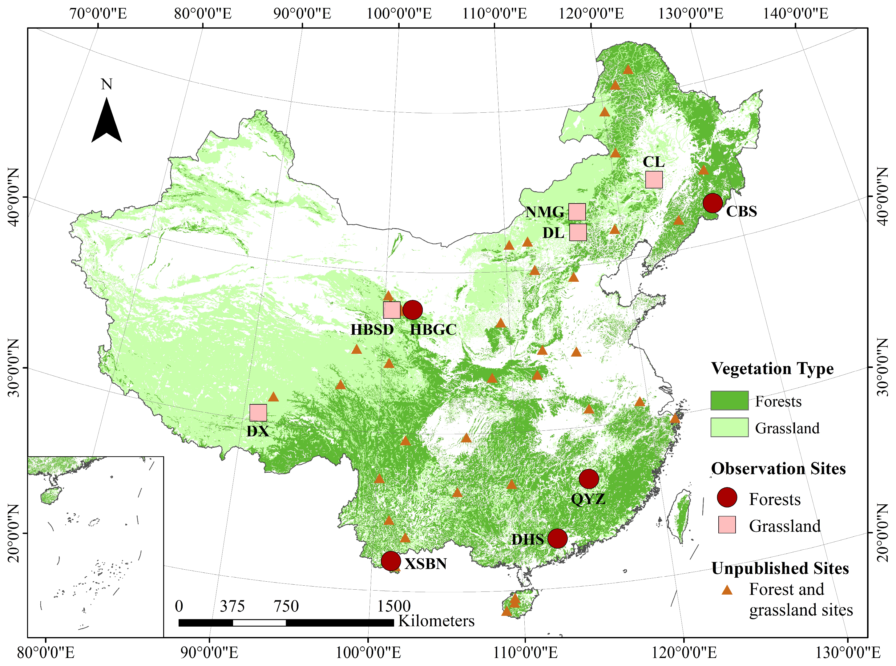
2.1. Study Area

In this study, we collected as much publicly available data as possible from forest and grassland flux sites in China. As shown in Figure 1, China has established 53 national forest and grassland flux observation sites, of which 10 sites have publicly available data, including 5 forest sites and 5 grassland sites. (The triangles in Figure 1 indicate forest and grass flux sites with unpublished data). The forest sites are Changbai Mountain (CBS), Haibei Shrubland (HBSL), Qianyanzhou (QYZ), Dinghu Mountain (DHS), and Xishuangbanna (XSBN). The grassland sites are Changling (CL), Inner Mongolia (NMG), Duolun (DL), Haibei (HBGL), and Dangxiong (DX). These 10 sites are highly representative of China, reflecting the country’s diverse vegetation and climate types. Additionally, they span a wide range of latitudes and longitudes, covering much of China’s temperature and precipitation gradients. The availability of publicly accessible flux observation data at these sites made them suitable for inclusion in this study. Detailed information on the latitude, longitude, elevation, vegetation type, and socio-economic (province) context of each site is provided in

Table 1. Description of flux observation sites.

Sites	Latitude (°, N)	Longitude (°, E)	Elevation (m)	Plant Functional Type	Annual Average Temperature (°C)	Precipitation (mm)	Provinces
CBS	42.40	128.10	738	DBF	3.6	713	Jilin
HBSL	37.61	101.32	3190	SHRUB	−1.2	535	Qinghai
QYZ	26.74	115.06	101	ENF	17.9	1542	Jiangxi
DHS	23.17	112.53	362	EBF	20.9	1956	Guangdong
XSBN	21.93	101.27	750	EBF	21.8	1493	Yunnan
CL	44.59	123.51	141	C3grass	4.9	470	Jilin
NMG	43.33	116.40	1200	C3grass	0.9	338	Inner Mongolia
DL	42.05	116.28	1317	C3grass	2.0	318	Inner Mongolia
HBGL	37.61	101.32	3202	C3grass	−1.1	490	Qinghai
DX	30.50	91.07	4332	C3grass	1.3	450	Tibet

.

2.2. Data Sources

2.2.1. Driving Data for the Biome-BGC Model

The Biome-BGC model requires the input of three key data types: geographical data, meteorological data, and ecophysiological parameters. Geographical data included the annual CO₂ concentration, soil texture, elevation, slope, and aspect. The CO₂ data required for the model were obtained from the publicly available annual monitoring data provided by the NOAA Global Monitoring Laboratory, located at the Mauna Loa Observatory in Hawaii. The data were accessed at https://www.co2.earth on 13 November 2022 [20]. Soil texture data were sourced from the China Soil Texture Spatial Distribution Dataset published by the Resource and Environment Science and Data Center, Chinese Academy of Sciences (https://www.resdc.cn/, accessed on 1 July 2024) [21]. Elevation, slope, and aspect data were obtained from the Chinese DEM distribution dataset also provided by the Resource and Environment Science and Data Center, Chinese Academy of Sciences (https://www.resdc.cn/, accessed on 1 July 2024) [21].

The meteorological data required to drive the Biome-BGC model included the daily maximum temperature (°C), daily minimum temperature (°C), average daily air temperature, daily total precipitation (cm), daily average water vapor pressure difference (Pa), and daily average global radiation (W/m²) [22]. These daily-scale meteorological data were derived using the MTCLIM model v4.3 at https://www.umt.edu/numerical-terradynamic-simulation-group/project/mt-clim.php, accessed on 23 August 2024 [23]. For this study, we selected data from nine national meteorological stations closest to the research sites to obtain daily-scale meteorological data from 1989 to 2008. These data were then used to drive the MTCLIM model to simulate the meteorological conditions for the ten study areas. The station numbers of the nine national meteorological stations are 54049, 54285, 54102, 54208, 52866, 55493, 57799, 59278, and 56969. The data from these stations were sourced from the China National Surface Weather Station Basic Meteorological Elements Daily Dataset (V3.0), provided by the China National Meteorological Information Center (http://data.cma.cn/, accessed on 13 November 2022) [24].

Ecophysiological parameters are also essential for driving the Biome-BGC model and typically include key plant functional traits such as the leaf carbon-to-nitrogen ratio and specific leaf area. In this study, the types of ecophysiological parameters that require assignment were determined by the results of a parameter sensitivity analysis based on the EFAST method. The values for sensitive ecophysiological parameters were derived from literature reviews and parameter optimization using PEST, while non-sensitive parameters were assigned the default values provided by the model. The parameters subjected to sensitivity analysis and their value ranges are detailed in Supplementary Materials S1, and the assigned values for the sensitive ecophysiological parameters for the ten study sites, along with their sources, are provided in Supplementary Materials S2.

2.2.2. Eddy Covariance Data

Eddy covariance systems, also known as flux towers, are among the most effective instruments for measuring carbon exchange between the atmosphere and various ecosystems. These systems provide direct measurements of ecosystem-level GPP and NEP [25,26]. In this study, all 10 representative forest and grassland ecosystems were equipped with flux towers. We obtained flux observation data from these 10 study sites for the years 2007 and 2008, including daily GPP and NEP measurements. The 2007 data were used for parameter optimization, while the 2008 data were utilized to validate the model’s simulation accuracy. These flux data were sourced from the China Flux Observation Network (Chinaflux, http://www.chinaflux.org/, accessed on 23 August 2024) [27] and the global Fluxnet 2015 dataset (https://fluxnet.org/data/fluxnet2015-dataset/, accessed on 13 November 2022) [28].

2.3. Biome-BGC Model

The BIOME-BGC model is a well-established ecosystem process model widely used both in China and globally due to its accurate depiction of carbon, nitrogen, and water cycles within forest and grassland ecosystems [13,29]. The BIOME-BGC model serves as a powerful tool for researchers to simulate vegetation ecosystem productivity, with numerous studies reporting its strong performance across various habitats worldwide [30,31,32]. The Biome-BGC model is capable of simulating four types of forest ecosystems (evergreen needleleaf, evergreen broadleaf, deciduous broadleaf, and deciduous needleleaf), two types of grasslands (C3 and C4 grasslands), and one type of shrubland. Through its detailed calculations of biogeochemical processes within vegetation ecosystems, the model generates a wide range of outputs, including GPP and NEP.

The BIOME-BGC model provides a detailed and precise depiction of material cycling and energy flow processes within ecosystems. Its core ecological processes include carbon fixation through photosynthesis, plant respiration and transpiration, leaf transpiration, soil water discharge, and runoff formation. The input data for the BIOME-BGC model comprise three main components: geographic data, meteorological data, and vegetation ecophysiological parameters [33]. The sources and processing methods for these data in this study are outlined in the previous sections. For a more comprehensive explanation of the operation and mechanisms of the Biome-BGC model, readers are referred to the relevant studies by Running et al. [33].

The Biome-BGC model was originally developed by Steve Running and has undergone several iterations under the maintenance of Peter Thornton [18,34]. The most recent official version of the model, Biome-BGC v4.2 is currently maintained by the Numerical Terradynamic Simulation Group (NTSG) at the University of Montana (http://www.ntsg.umt.edu/project/biome-bgc.php, accessed on 23 August 2024) [23]. The version utilized in this study is also Biome-BGC v4.2.

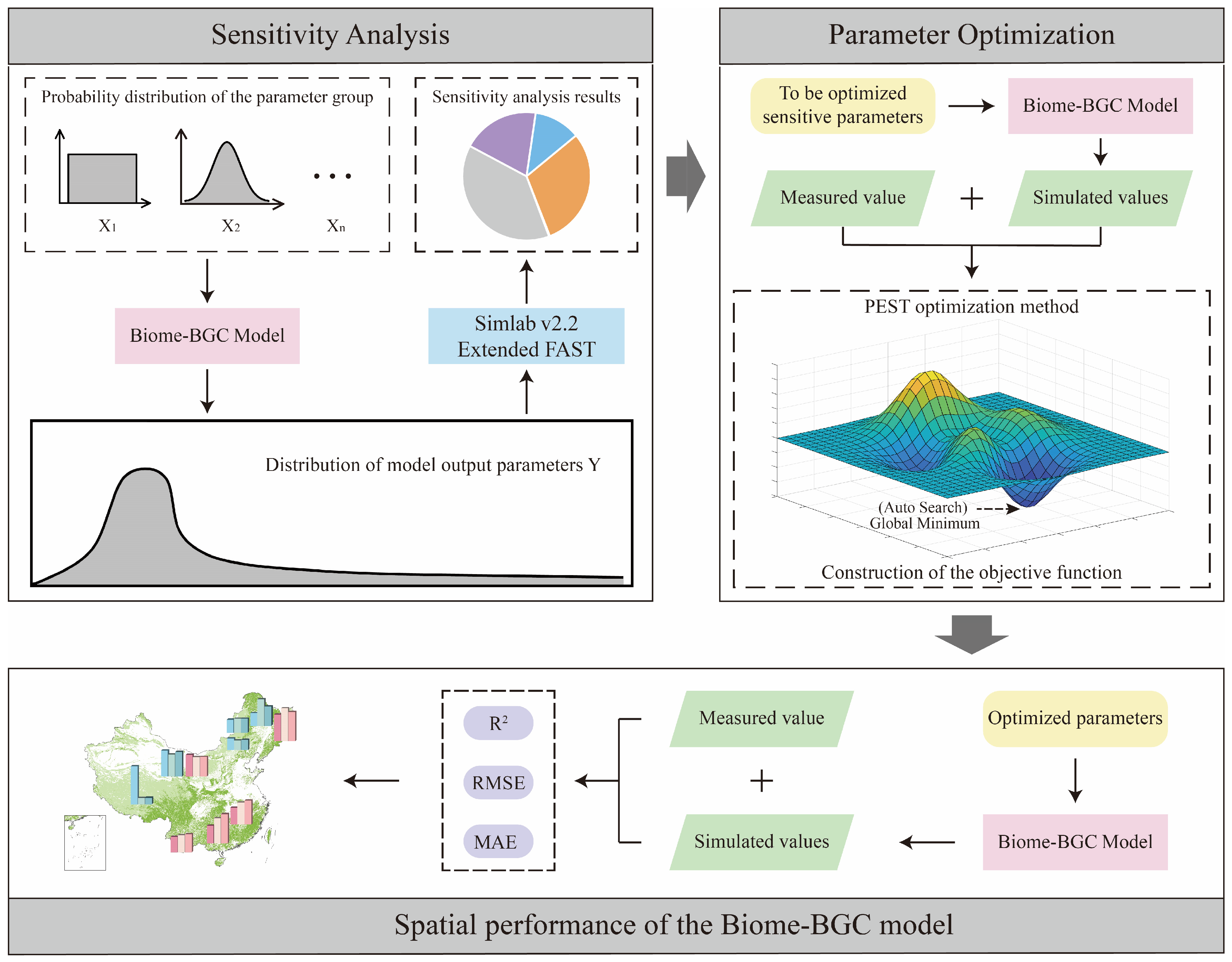
2.4. Sensitivity Analysis

Sensitivity analysis is a crucial step in the calibration process of the model parameters [35], which serves to evaluate the influence of each parameter in the model on the output results. The EFAST method is often used by researchers for sensitivity analysis in Biome-BGC models [11,12,13]. In this study, the EFAST method was adopted for the sensitivity analysis of the Biome-BGC model to quantify the contribution of input parameters to GPP and NEP, filtering out the parameters that have a high influence on the model output results for subsequent parameter optimization. EFAST is a global sensitivity analysis method proposed by Saltelli based on the Fourier amplitude sensitivity test (FAST) method combined with Sobol’s method [36,37,38]. This method is based on variance theory, which considers that the output results of the model are not only influenced by the parameters themselves but also correlated with the interactions between parameters. Through the decomposition of the variance, the contribution to the total variance is generated by the independent and mutual coupling of parameters, respectively, namely, the sensitivity index.

EFAST defines the total variance of the model outputs as the sum of the model parameters themselves and the interactions between their different parameters, as shown in Equation (1) [39]:

$$V_Y=\sum _i{V}_i+\sum _i\sum _{j>i}{V}_{ij}+\sum _i\sum _{j>i}\sum _{k>j}{V}_{ijk}+\cdots +V_{12\cdots n}$$

(1)

where V_Y is the total variance of the model output; V_i is the variance of individual factors; and V_ij~V_(12…n) is the variance of interactions between parameters.

The total order index (S_iT) of parameter X_i is the sum of the first-order sensitivity index (S_i) of the parameter and each order sensitivity index of the parameter in interaction with other parameters, which can be represented as [39]:

$$S_{iT}=S_i+S_{ij}+\cdots +S_{12\cdots i\cdots n}$$

(2)

where S_i = V_i/V_Y is the direct contribution of parameter X_i to the total variance of the model output results, namely, the first-order sensitivity index; S_ij = V_ij/V_Y is the influence degree of the interaction between parameters X_i and X_j on the output results of the model, namely, the second-order sensitivity index, and so on.

Here, we conducted a sensitivity analysis for the ecophysiological parameters of the model, which was implemented with the EFAST module of the sensitivity and uncertainty analysis software SimLab 2.2. In accordance with the fluctuation range of the input parameters, the Monte Carlo method was used to randomly sample each parameter [40], and we set the number of samples for each parameter to 130. (EFAST prescribes that the number of samples for each parameter should be more than 65.) The Biome-BGC model was executed in batches according to the generated input parameters. After that, we simulated the GPP and NEP over 30 years (1989–2018) and calculated the average value of multiple years, which were input to SimLab to obtain the sensitivity index of each parameter. Based on the total order index ranking, we divided the parameters into two groups. Among them, the top five parameters in the ranking of the total order index were the sensitive parameters; otherwise, they were insensitive parameters. Additionally, the key sensitivity parameters were those ranked in the top five for both the total order index and the first-order sensitivity index.

2.5. Parameter Optimization

The PEST method (model-independent parameter estimation and uncertainty analysis) is a nonlinear parameter optimization tool that operates independently of the model itself [41]. Initially developed for parameter optimization in groundwater models, it has since been widely adopted by researchers for calibrating the optimal values of ecophysiological parameters in the Biome-BGC model [10,13,42,43,44]. The PEST optimization method can be used for the global optimization of ecophysiological parameters, which can take into account the interaction between parameters in the optimization process and can optimize multiple parameters simultaneously with high optimization efficiency [45,46]. The model is built on the Gauss–Marquardt–Levenberg (GML) algorithm, which adjusts the input parameters of the tuned model through several iterations, and eventually minimizes the difference between the output value of the tuned model and the actual observed value [47]. Its core algorithm is to seek the minimum value of the objective function (the difference function between the simulated and measured values of the model) [48]. In this study, the output results of parameter optimization were GPP and NEP, so the PEST algorithm objective function is represented as [49,50,51]:

$$\mathsf{\Psi }\left(\mathrm{F}\right)={\mathsf{\Psi }}_{\mathrm{G}\mathrm{P}\mathrm{P}}+{\mathsf{\Psi }}_{\mathrm{N}\mathrm{E}\mathrm{P}}=\sum _{i=1}^{n_1}{w^2}_{\mathrm{G}\mathrm{P}\mathrm{P},i}{\left({obs}_{\mathrm{G}\mathrm{P}\mathrm{P},i}-{sim}_{\mathrm{G}\mathrm{P}\mathrm{P},i}\right)}^2+\sum _{i=1}^{n_2}{w^2}_{\mathrm{NEP},i}{\left({obs}_{\mathrm{N}\mathrm{E}\mathrm{P},i}+{sim}_{\mathrm{N}\mathrm{E}\mathrm{P},i}\right)}^2$$

(3)

where $\mathsf{\Psi }\left(\mathrm{F}\right)$ is the objective function of the parameter set F to be parametrically optimized; obs is the actual observed value of the flux observation site; sim is the simulated value of the Biome-BGC model; w is the weight coefficient set for the observation; i is the time, which denotes the yearday (namely the ith day of the year) of the Biome-BGC model in this study; $n_1$ and $n_2$ are the number of the observed data, which is the number of daily scale flux observations in this study, with a value of 365; and the subscripts GPP and NEP are gross primary productivity and net ecosystem productivity, respectively.

In the course of the calibration of optimal values of the missing measurement sensitivity parameters using the PEST method, we used the flux observed by GPP and NEP in 2007 for parameter optimization and the flux observations of GPP and NEP in 2008 for accuracy verification. This study was performed based on the latest version of PEST 17.3, and the model principles and applicability are detailed in the operational guide (http://www.pesthomepage.org/, accessed on 13 November 2022) [51].

2.6. Evaluation of Simulation Accuracy

In this study, three statistical indicators were chosen to evaluate the modification of the simulation accuracy of the Biome-BGC model before and after the optimization of the parameters of the PEST method, which are the coefficient of determination (R²), the root mean square error (RMSE), and the mean absolute error (MAE). It can be represented mathematically as [52,53]:

$$R^2={\left[{\displaystyle \frac{{\sum }_{i=1}^n\left(S_i-\overline{S}\right)\left(O_i-\overline{O}\right)}{\sqrt{{\sum }_{i=1}^n{\left(S_i-\overline{S}\right)}^2{\left(O_i-\overline{O}\right)}^2}}}\right]}^2$$

(4)

$$\mathrm{R}\mathrm{M}\mathrm{S}\mathrm{E}=\sqrt{{\displaystyle \frac{1}{n}}{\sum }_{i=1}^n{\left(S_i-O_i\right)}^2}$$

(5)

$$\mathrm{M}\mathrm{A}\mathrm{E}={\displaystyle \frac{1}{n}}{\sum }_{i=1}^n\left|S_i-O_i\right|$$

(6)

where $S_i$ is the simulated value of the model on the $i$th day; $O_i$ is the observed value of the flux on the $i$th day; $\overline{S}$ and $\overline{O}$ are the average values of the simulated and observed values, respectively; and $n$ is the total number of days of the model simulation.

We used $R^2$ to evaluate the degree of fit of the Biome-BGC model and the RMSE and MAE to evaluate the deviance between the simulated values of the Biome-BGC model and the observed fluxes. $R^2$ was obtained by linear regression between the simulated values of the model and the observed fluxes, reflecting the ability of the simulated values to match the variation in the observed values. It is concerned with the closeness of the change trends of these two curves, emphasizing whether the changes of simulated and observed values are in the same direction. The closer the value to 1 indicates the better the fit of the simulation results to the measured results. The RMSE was used to evaluate the difference between the simulated and measured values. It penalizes extremely poor predictions and amplifies the difference between simulated and observed values with large deviations. It is more sensitive to abnormal values in the simulations, where smaller values indicate less discrepancy between simulated and measured results. The MAE is the average of the absolute errors between simulated and observed values, and its contribution per error to the MAE is proportional to the absolute value of the error, reflecting the actual error between each set of simulated and observed values. In contrast to the RMSE, which involves squaring the errors, some relatively large errors will cause the RMSE to increase more than the MAE.

2.7. Technical Route of This Study

The technical route of this study consists of three components: a sensitivity analysis of the ecophysiological parameters, parameter optimization, and a spatial evaluation of model accuracy. To identify the sensitive ecophysiological parameters within the Biome-BGC model that are crucial for subsequent parameterization and optimal value calibration, we initially applied the EFAST method to analyze the sensitivity of these parameters across ten representative forest and grassland ecosystems. Upon identifying the parameters with significant influence on the simulation outcomes, we assigned values to them based on empirically measured data reported in the literature. For those sensitive parameters for which empirical data could not be obtained from the literature, we employed the PEST method to determine their optimal values. Subsequently, the Biome-BGC model was driven by these parameterized values to simulate GPP and NEP across the ten ecosystems. The model’s accuracy was then spatially evaluated using three indicators: the R², RMSE, and SAE. Finally, we derived the spatial pattern of the Biome-BGC model’s simulation accuracy across China’s representative forest and grassland ecosystems. The overall technical route is illustrated in Figure 2.

3. Results

3.1. Sensitivity Analysis of Ecophysiological Parameters

In this study, we conducted a sensitivity analysis of the ecophysiological parameters of the Biome-BGC model across 10 sites using the EFAST method. We identified the parameters with the greatest impact on the simulation results of GPP and NEP by evaluating the sensitivity indices, including the first-order sensitivity index (S_i) and the total sensitivity index (S_iT). The sensitivity analysis results for the 10 sites are presented in Figure 3, and the complete sensitivity ranking of all parameters is provided in Supplementary Materials S3.

S_i (first-order sensitivity index) represents the direct contribution of a parameter to the model’s simulation results, while S_iT (total sensitivity index) reflects the overall contribution of a parameter, including its interactions with other parameters [54]. The sensitivity analysis of the Biome-BGC model for GPP simulation reveals that the S_i and S_iT results were largely consistent. This suggests that the ecophysiological parameters of the Biome-BGC model primarily influence the simulation results directly, with minimal interaction among them. Additionally, in the GPP simulations, the parameters with the highest sensitivity index values included FLNR (fraction of leaf N in Rubisco), C:N_leaf (C:N of leaves), k (canopy light extinction coefficient), G_smax (maximum stomatal conductance), and C:N_fr (C:N of fine roots). This indicates that these parameters are frequently the most sensitive, significantly impacting the Biome-BGC simulation results. Notably, FLNR exhibited the highest sensitivity index value during GPP simulation at the HBSL site.

The results of the parameter sensitivity analysis of the Biome-BGC model in simulating NEP show that the parameters with larger values of S_i were FLNR, k, and C:N_leaf. The parameters with larger values of S_iT were FLNR, C:N_fr, LWP_f (leaf water potential), and DW_cel (dead wood cellulose proportion). Additionally, the S_iT values for nearly all parameters are greater than their S_i values, and the parameters with high S_iT values differ from those with high S_i values. This suggests that during NEP simulation, the ecophysiological parameters in the Biome-BGC model interact extensively with one another, collectively influencing the simulation results. The reason for this phenomenon is that the ecophysiological processes carried out by the Biome-BGC model when simulating NEP are more complex than when simulating GPP, and more mathematical formulas are applied to the model’s calculations at the same time that more ecophysiological parameters interact with each other. For example, simulating NEP requires additional calculations of plant autotrophic respiration and soil respiration compared to simulating GPP.

Overall, factors such as spatial distribution, plant functional types, and the model output metrics (GPP or NEP) contribute to changes in the sensitivity of the ecophysiological parameters within the Biome-BGC model. These changes are irregular and complex, making them difficult to predict without conducting parameter sensitivity analyses.

3.2. Calibration of Optimal Values for Sensitive Ecophysiological Parameters

In this study, we utilized a literature review and the PEST method to calibrate the optimal values for sensitivity-related ecophysiological parameters of the Biome-BGC model across 10 representative forest and grassland ecosystems. We gathered and reviewed a substantial amount of research on these parameters, prioritizing the observed values reported in the literature for calibration. For parameters not covered in the literature, we applied the PEST method to determine the optimal values (results are shown in Supplementary Materials S4). During the parameter optimization process, carbon flux observations from 2007 at these 10 typical vegetation sites in China were used as the benchmark for model validation. Following parameter optimization, carbon flux observations from 2008 were employed to assess the simulation accuracy of the model. The results, illustrating the extent of improvement in the simulation accuracy of the Biome-BGC model at these 10 sites post-optimization, are shown in Figure 4.

Overall, the regression analysis of the simulated and observed carbon fluxes from the Biome-BGC model shows that the R² (coefficient of determination) for both GPP (gross primary productivity) and NEP (net ecosystem productivity) improved following parameter optimization, while the RMSE and MAE of GPP and NEP decreased at most observation stations. This indicates that parameter optimization enhanced the simulation accuracy of the Biome-BGC model for both GPP and NEP at these 10 stations. Specifically, for the GPP simulation, the site with the most significant R² improvement after parameter optimization was HBSL, where the R² increased from 0.38 to 0.81, reflecting an improvement of 53.09%. The DHS site showed the largest reduction in the RMSE and MAE, with decreases of 65.42% and 68.50%, respectively. For the NEP simulation, HBSL again exhibited the greatest R² improvement, with a remarkable increase of 99.84%. The XSBN site had the largest reductions in the RMSE and MAE, with decreases of 55.32% and 57.35%, respectively.

The increase in the R² indicates that, after parameter optimization, the Biome-BGC model can more accurately simulate the temporal variations in productivity (including GPP and NEP). The decrease in the RMSE and MAE suggests that parameter optimization brings the Biome-BGC model’s simulation results closer to the observed values. For instance, as shown in Figure 4, the regression analysis of GPP after parameter optimization demonstrates a significant improvement in the accuracy of the model’s time-series simulations at the HBSL, XSBN, and DHS sites. Additionally, the numerical error in GPP simulations at the QYZ, DHS, and XSBN sites is greatly reduced. In summary, parameter optimization has enhanced the simulation accuracy of the Biome-BGC model at the vast majority of the 10 sites examined in this study.

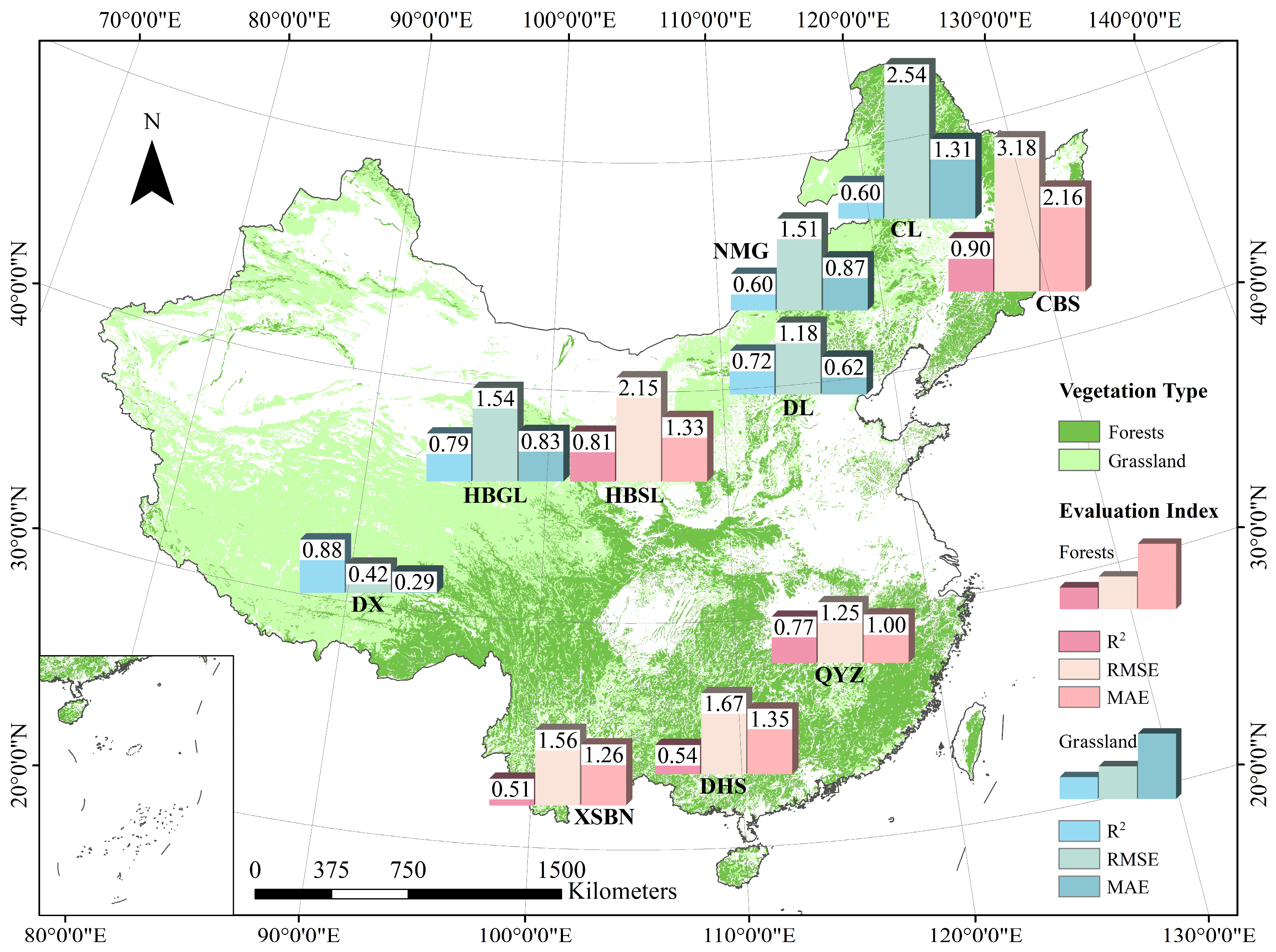
3.3. Spatial Pattern of Biome-BGC Model Applicability in China

In this study, we combined regression analysis with three model accuracy evaluation indices (the R², RMSE, and SAE; see Section 2.6) to quantitatively assess the simulation accuracy of the parameter-optimized Biome-BGC model across 10 typical ecosystems in China. We then explored the spatial distribution pattern of the model’s applicability across the country. The spatial distribution of the Biome-BGC model’s simulation accuracy for GPP (gross primary productivity) and NEP (net ecosystem productivity) at the 10 sites is shown in Figure 5 and Figure 6. As observed from Figure 5 and Figure 6, the R² (coefficient of determination) for GPP at all sites ranged from 0.51 to 0.90, while for NEP, it ranged from 0.19 to 0.63. This indicates that the Biome-BGC model exhibited a better fit for GPP than for NEP.

The simulation accuracy of GPP based on the Biome-BGC model for 10 typical ecosystems in China shows that the R² values for the five forest sites (XSBN, DHS, QYZ, HBGC, and CBS) increased sequentially, with values of 0.51, 0.54, 0.77, 0.81, and 0.90, respectively. This indicates that for forest ecosystems in China, the goodness of fit of the Biome-BGC model gradually improves with increasing latitude (Figure 5). Meanwhile, the MAE values for XSBN, DHS, QYZ, and HBSL were relatively close to each other, while the MAE value for CBS was larger than that of the other four forest sites. In other words, the RMSE and MAE of the five forest sites did not exhibit a specific spatial pattern with latitude. However, when considering the R², RMSE, and MAE results together, the accuracy of GPP simulation for Chinese forest ecosystems using the Biome-BGC model gradually increases with increasing latitude.

For grassland ecosystems in China, the GOP (goodness of fit) at the five grassland sample sites (DX, HBGL, DL, NMG, and CL) decreased sequentially with increasing latitude, with the R² values of 0.88, 0.79, 0.72, 0.60, and 0.60, respectively. This means that the variability pattern of the Biome-BGC model’s goodness of fit (GPP) for grassland ecosystems along the latitudinal gradient was opposite to that observed for forest ecosystems. Meanwhile, the MAEs for the five grassland sites (DX, HBGL, DL, NMG, and CL) were 0.29, 0.83, 0.62, 0.87, and 1.31, indicating that as latitude increases, the overall trend in model simulation error for the five grassland sites shows an upward trend. Combining the R² and MAE results for the five grassland sites, it is evident that the GPP simulation accuracy of the Biome-BGC model for grassland ecosystems in China gradually decreases with increasing latitude.

Similarly, the NEP simulation accuracy for 10 typical Chinese ecosystems based on the Biome-BGC model shows that the R² values for the five forest sites (XSBN, QYZ, DHS, HBGC, and CBS) increased sequentially, with values of 0.31, 0.33, 0.35, 0.43, and 0.52, respectively. This indicates that for forest ecosystems in China, the goodness of fit of the Biome-BGC model gradually improves with increasing latitude (Figure 6). Meanwhile, the MAE values for XSBN, DHS, QYZ, and HBSL were relatively close to each other, while the MAE value for CBS was larger than that of the other four forest sites. In other words, the RMSE and MAE of the five forest sites did not exhibit a specific spatial pattern with latitude. However, when considering the R², RMSE, and MAE results together, the accuracy of NEP simulation for Chinese forest ecosystems using the Biome-BGC model gradually increases with increasing latitude.

For grassland ecosystems in China, the GOP (goodness of fit, GOP) at the five grassland sample sites (DX, HBGL, DL, NMG, and CL) decreased sequentially with increasing latitude, with the R² values of 0.63, 0.43, 0.19, 0.21, and 0.21, respectively. This means that the variability pattern of the Biome-BGC model’s goodness of fit (GPP) for grassland ecosystems along the latitudinal gradient was opposite to that of forest ecosystems. Meanwhile, the MAEs for the five grassland sites (DX, HBGL, DL, NMG, and CL) were 0.25, 0.91, 0.38, 0.51, and 0.72, indicating that as latitude increases, the overall trend in model simulation error for the five grassland sites increases. When combining the R² and MAE results for the five grassland sites, it becomes evident that the NEP simulation accuracy of the Biome-BGC model for grassland ecosystems in China gradually decreases with increasing latitude.

By analyzing the accuracy of the Biome-BGC model in simulating the productivity of 10 typical Chinese ecosystems (5 forest ecosystems and 5 grassland ecosystems), we found that the simulation results of GPP and NEP exhibited an overall consistent pattern. This consistency suggests that the model is capable of accurately simulating the process of ecosystem carbon cycling, demonstrating a certain degree of simulation accuracy and reliability.

4. Discussion

4.1. Uncertainty of Parameter Sensitivity

The results of EFAST show different vegetation types vary in terms of sensitive parameters. Parameter sensitivity tests were performed for HBSL and HBGL sites located at the same latitude and longitude in the study, resulting in different combinations of sensitive parameters. On the one hand, the input parameters required for different PFTs are not exactly the same. There are more constant parameters for grass in the EPC file supplied by the developer, such as LWT (annual live wood turnover fraction) and SC:LC (new stem C/new leaf C). As grasslands have no woody stems, these parameters only need to be provided to the shrub or forest site; therefore, no sensitivity analysis is required for these parameters at the grassland site. On the other hand, it might be correlated with the differences in the photosynthetic properties of different PFTs, which lead to different sensitivities of the photosynthesis-related parameters for grassland and shrubs [55]. Take for example FLNR, which determines the magnitude of the maximum carboxylation rate in the model photosynthesis module [56], and the Rubisco enzyme directly affects the first step of the vegetation fixation of atmospheric CO₂. This explains the fact that FLNR is a sensitive parameter for HBSL and not for HBGL. However, the climate and environmental conditions varied under different latitudes and longitudes, and the sensitive parameters of the same vegetation type were not the same, as at all nonwoody sites in this paper. This might be attributed to the significant variation in plant traits along the climatic zone and the relative reduction in the degree of influence when the parameters are no longer limited by hydrothermal conditions. Additionally, we found that the parameter sets sensitive to GPP and NEP were not identical for the same PFTs at the same site. It is a more complicated process to calculate NEP compared to GPP. Gross primary productivity (GPP) minus the part consumed by vegetation respiration and the part consumed by heterotrophic respiration (soil respiration) is the net ecosystem productivity (NEP), which involves processes such as C and N cycles, the autotrophic (maintenance and growth) stage and the heterotrophic (decomposition) stage of the Biome-BGC model. As a result, the different geochemical cycling processes involved in GPP and NEP may have contributed to the difference in the sensitivity of different definitions of plant productivity to the same parameter.

Through a comprehensive analysis of the existing studies [12,57], when researchers selected sensitive parameters using different methods (annealing algorithms and the Morris method, etc.), they obtained not completely identical results. One study conducted a sensitivity analysis of the parameters of the Biome-BGC model with the Morris method and EFAST method, respectively [58]. The parameters’ nascent fine-root-to-leaf carbon partition ratio and fine-root carbon-to-nitrogen ratio were screened as sensitive parameters by EFAST, while in the Morris method, they were not. In addition, researchers have set different thresholds for dividing sensitive parameters. For example, some researchers have considered parameters with a total sensitivity index greater than 0.05 as influential parameters in the parameterization of the Biome-BGC model [59]. Other researchers have divided the sensitivity index into three categories in sensitivity analysis when using the Biome-BGC model to simulate forest carbon fluxes, namely, strong-effect parameters (>0.2), medium-effect parameters (>0.1 and ≤0.2), and low-effect parameters (≤0.1) [29]. The diversity of the threshold classification standards leads to different types and numbers of sensitive parameters screened.

To summarize, the uncertainty of model sensitivity parameters originates from many aspects, including the type of vegetation at the study site, the spatial location, the output variables of the model (GPP, NPP, or NEP), and different sensitivity analysis methods. Consequently, when we need to simulate carbon fluxes in a new study area using the Biome-BGC model, it is necessary to perform sensitivity analysis for the region as well as the different carbon fluxes simulated.

4.2. The Latitude Pattern of Model Applicability and Its Reasons

Most of the uncertainties in carbon flux simulations are derived from the model structure and input parameters, which lead to biased modeling results. In this study, the optimal values of parameters were calibrated through a uniform model parameterization process, and the spatial variability in the accuracy of the Biome-BGC model simulation productivity was analyzed. We found that the simulation ability of the Biome-BGC model probably has greater differences in the north and south of China.

In forest ecosystems, there is a noticeable decline in model simulation accuracy from northern to southern China. This pattern is also observed in the study by Liu [16]. The R² value of 0.57 for the original simulated NEP at the HF and CBS sites with higher latitudes is more accurate (with an R² value of 0.18) compared to the simulations at the QYZ and DHS sites in southern China. Among the five forest nodes in this paper, the model simulates vegetation productivity with the lowest accuracy in XSBN, which fails to fit well even after parameter optimization. (The R² value of GPP is 0.51, and the R² value of NEP is 0.31.) From the perspective of the distribution characteristics of forests, this is likely because of the high diversity of species and the high complexity of forest community composition in the south compared to the north. However, the Biome-BGC model lacks generalized default parameters for mixed forests and can only simulate the productivity of idealized pure forests (single PFTs). Due to the unsuitability of the ecophysiological parameters for southern forest vegetation, the model’s simulation accuracy is low in the southern regions. The Biome-BGC model exhibits a consistent spatial pattern in its simulation accuracy across typical forest ecosystems in China along a latitudinal gradient. However, latitude inherently influences gradients in temperature and precipitation. In China, annual precipitation and mean annual temperature increase from north to south as latitude decreases. For forest ecosystems, the forests in lower latitude regions are typically located in subtropical or tropical climate zones, characterized by higher average temperatures and greater annual precipitation. Through daily analysis of meteorological data used by the Biome-BGC model for productivity simulations at the XSBN and DHS sites, we found that during periods of extended drought within the peak growing season, the model significantly overestimated evapotranspiration and soil runoff. This led to water stress within the forest ecosystems, negatively impacting the photosynthesis module and consequently reducing the accuracy of GPP and NEP simulations. This phenomenon has also been reported in other studies [60,61].

In grassland ecosystems, the accuracy of model simulations exhibits a clear increasing trend from northern to southern China. This result may be attributed to the design of most ecophysiological processes in the Biome-BGC model, which is referenced from coniferous forest ecosystems [33]. Consequently, the model fails to accurately depict the key ecophysiological processes of grassland ecosystems, thereby limiting its ability to fit the maximum productivity of grasslands. Through the analysis of multiple processes (carbon cycle, nitrogen cycle, and water cycle) within the model, we found that the simulation intensity of the water cycle processes, such as evapotranspiration and outflow, in the Biome-BGC model is greater than the actual situation. This creates a false impression of water stress. As a result, the simulation intensity of photosynthesis in grassland ecosystems is lower than the actual condition, ultimately leading to an error where the simulated maximum productivity at a daily scale during the growing season is lower than reality. Due to the spatial pattern of increasing precipitation and temperature from north to south in China, the hydrothermal conditions for northern grasslands are poorer than those for southern grasslands. Therefore, northern grasslands are more susceptible to deficiencies in the water cycle module of the model. This has also been confirmed in a study by Cheng [62].

In addition to moisture and temperature, the elevation of forest and grassland ecosystems may also affect the simulation accuracy of the Biome-BGC model. Within the Biome-BGC model’s mechanistic processes, elevation determines atmospheric pressure, which, in turn, influences the concentration of oxygen in the atmosphere. Oxygen concentration can affect the carboxylation rate of plant photosynthesis, potentially impacting the model’s outputs of GPP and NEP [22]. Given the significant variation in elevation among the ten sites studied, without a clear gradient, it is challenging to explore the relationship between elevation and the Biome-BGC model’s simulation accuracy. We plan to investigate this issue further in future research.

4.3. Suggestions for Using the Original Biome-BGC Model in China and Future Research Directions

As described in Section 3.3 of this study, the applicability of the Biome-BGC model has spatial variability in China, where the accuracy of simulations decreases from north to south for woody sites and increases from north to south for nonwoody sites. In other words, the model has high simulation accuracy in high-latitude forests (such as the CBS site) or low-latitude grasslands (such as the DX site) in China. Both the GPP and NEP daily trends are well matched by the model at these sites, even without parameter optimization. Therefore, when using the original Biome-BGC model to simulate forest productivity in northern China or grassland productivity in southern China, we propose that rigorous parameter optimization may be unnecessary to obtain good simulation results. When simulating forest productivity in the south or grassland productivity in the north, sensitivity analysis and parameter optimization probably have little improvement in simulation accuracy because of the limitations of the model structure. It may be necessary to assimilate data or target some modules of the model to improve the accuracy of the simulation.

The implication for practical management is that forest (or grassland) management managers can use the original Biome-BGC model when using productivity pairs to assess the growth status and management level in northern forests or southern grasslands in China, while directly using the model would lead to larger errors for estimating the forest productivity in northern China or grassland productivity in southern China.

The simulation accuracy of the Biome-BGC model is greatly improved after parameter optimization but is still not excellent in southern forests and northern grasslands. In other words, there is a large promotion space for the simulation accuracy of the model in southern forests and northern grasslands. From a side view, the reason for the lower simulation accuracy of the Biome-BGC model in southern forests and boreal grasslands probably originates from the incompatibility and absence of structural and mechanistic processes in the model. For example, the ecophysiological parameters entered in the Biome-BGC model are in static form, while the previous study revealed that the optimal values of the parameters are variable in time series [11]. Both specific leaf area (SLA) and leaf carbon to nitrogen ratio (C:Nleaf) are important parameters of plant photosynthesis links, whereas they are input to the model in the form of fixed values. As a result, the parameters do not match in temporal resolution and mechanism, thus making the leaf area index (LAI) simulated by the model at the site differ from the actual one. In this regard, a researcher has already input the LAI obtained from remote sensing data into the model using data assimilation and obtained better simulation results [16]. Accordingly, we can modify the parameter with a large variation in the optimal value on the time series, changing the individual input values to a series of input values that vary with month, season, or phenological period. With the improved structure of the model, researchers eliminate the need for data assimilation, which greatly improves the efficiency and accuracy of the simulation and lowers the threshold of use. The future direction is, therefore, to improve the mechanistic process of the Biome-BGC model in more depth and its simulation accuracy in southern forests and northern grasslands in China.

Additionally, this study has certain limitations. Due to the limited availability of publicly accessible flux observation data, the number of study sites in this research is relatively small compared to the national flux stations in China. As more national-level flux observation data become available in the future, we will be able to include more study sites, thereby making the spatial pattern of the Biome-BGC model’s simulation accuracy more representative and convincing. Furthermore, this study did not select research sites based on an elevation gradient to explore the relationship between elevation and the Biome-BGC model’s simulation accuracy. We plan to conduct further research in this direction in the future.

5. Conclusions

In this study, we focused on ten vegetative ecosystems in China with established flux observation stations. Using the EFAST method, we identified the key sensitive ecophysiological parameters of the Biome-BGC model and calibrated their values, subsequently analyzing the model’s simulation accuracy across these ten ecosystems. This study elucidates the spatial variability in the simulation accuracy of the Biome-BGC model in China, revealing its spatial applicability in Chinese vegetative ecosystems and providing a set of locally calibrated vegetation ecophysiological parameters for the Biome-BGC model. The results indicate that for forest ecosystems, the simulation accuracy of the Biome-BGC model shows a decreasing trend from northern to southern China. Conversely, for grassland ecosystems, the simulation accuracy exhibits an increasing trend from north to south. Furthermore, the types of sensitive ecophysiological parameters of the Biome-BGC model vary with the spatial location of the simulation object, vegetation type, and output indicators. Therefore, we emphasize that the use of the Biome-BGC model should be based on parameter sensitivity analysis and optimization, with greater attention to the spatial variability of model applicability.

References

1. Fang, J.; Yu, G.; Liu, L.; Hu, S.; Chapin, F.S. Climate Change, Human Impacts, and Carbon Sequestration in China. Proc. Natl. Acad. Sci. USA 2018, 115, 4015–4020. [Google Scholar] [CrossRef] [PubMed]
2. Fang, M.; Si, G.; Yu, Q.; Huang, H.; Huang, Y.; Liu, W.; Guo, H. Study on the Relationship between Topological Characteristics of Vegetation Ecospatial Network and Carbon Sequestration Capacity in the Yellow River Basin, China. Remote Sens. 2021, 13, 4926. [Google Scholar] [CrossRef]
3. Fang, J.; Ke, J.; Tang, Z.; Chen, A. Implications and estimations of four terrestrial productivity parameters. Acta Phytoecol. Sin. 2001, 25, 414–419. [Google Scholar]
4. Lu, F.; Hu, H.; Sun, W.; Zhu, J.; Liu, G.; Zhou, W.; Zhang, Q.; Shi, P.; Liu, X.; Wu, X.; et al. Effects of National Ecological Restoration Projects on Carbon Sequestration in China from 2001 to 2010. Proc. Natl. Acad. Sci. USA 2018, 115, 4039–4044. [Google Scholar] [CrossRef]
5. Li, X.; Ma, H.; Ran, Y.; Wang, X.; Zhu, G.; Liu, F.; He, H.; Zhang, Z.; Huang, C. Terrestrial Carbon Cycle Model-Data Fusion: Progress and Challenges. Sci. China Earth Sci. 2021, 64, 1645–1657. [Google Scholar] [CrossRef]
6. Fang, M.; Cheng, C.; He, N.; Si, G.; Sun, O.J. Implication of Community-Level Ecophysiological Parameterization to Modelling Ecosystem Productivity: A Case Study across Nine Contrasting Forest Sites in Eastern China. J. For. Res. 2024, 35, 7. [Google Scholar] [CrossRef]
7. Su, H.; Sang, W.; Wang, Y.; Ma, K. Simulating Picea Schrenkiana Forest Productivity under Climatic Changes and Atmospheric CO2 Increase in Tianshan Mountains, Xinjiang Autonomous Region, China. For. Ecol. Manag. 2007, 246, 273–284. [Google Scholar] [CrossRef]
8. Wu, Y.; Wang, X.; Ouyang, S.; Xu, K.; Hawkins, B.A.; Sun, O.J. A Test of BIOME-BGC with Dendrochronology for Forests along the Altitudinal Gradient of Mt. Changbai in Northeast China. J. Plant Ecol. 2017, 10, 415–425. [Google Scholar] [CrossRef]
9. Luo, Z.; Sun, O.J.; Wang, E.; Ren, H.; Xu, H. Modeling Productivity in Mangrove Forests as Impacted by Effective Soil Water Availability and Its Sensitivity to Climate Change Using Biome-BGC. Ecosystems 2010, 13, 949–965. [Google Scholar] [CrossRef]
10. Wen, Y.; Han, H.; Cheng, X.; Li, Z. Forest water use efficiency in Qianyanzhou based on Biome-BGC model, Jiangxi Province of eastern China. J. Beijing For. Univ. 2019, 41, 69–77. [Google Scholar] [CrossRef]
11. Li, Y.Z.; Zhang, T.L.; Liu, Q.Y.; Li, Y. Temporal and spatial heterogeneity analysis of optimal value of sensitive parameters in ecological process model: The BIOME-BGC model as an example. Ying Yong Sheng Tai Xue Bao 2018, 29, 84–92. [Google Scholar] [CrossRef] [PubMed]
12. Ren, H.; Zhang, L.; Yan, M.; Tian, X.; Zheng, X. Sensitivity Analysis of Biome-BGCMuSo for Gross and Net Primary Productivity of Typical Forests in China. For. Ecosyst. 2022, 9, 100011. [Google Scholar] [CrossRef]
13. Sun, J.; Mao, F.; Du, H.; Li, X.; Xu, C.; Zheng, Z.; Teng, X.; Ye, F.; Yang, N.; Huang, Z. Improving the Simulation Accuracy of the Net Ecosystem Productivity of Subtropical Forests in China: Sensitivity Analysis and Parameter Calibration Based on the BIOME-BGC Model. Forests 2024, 15, 552. [Google Scholar] [CrossRef]
14. Zhang, T.; Sun, R.; Peng, C.; Zhou, G.; Wang, C.; Zhu, Q.; Yang, Y. Integrating a Model with Remote Sensing Observations by a Data Assimilation Approach to Improve the Model Simulation Accuracy of Carbon Flux and Evapotranspiration at Two Flux Sites. Sci. China Earth Sci. 2016, 59, 337–348. [Google Scholar] [CrossRef]
15. Yan, M.; Tian, X.; Li, Z.; Chen, E.; Wang, X.; Han, Z.; Sun, H. Simulation of Forest Carbon Fluxes Using Model Incorporation and Data Assimilation. Remote Sens. 2016, 8, 567. [Google Scholar] [CrossRef]
16. Liu, Q.; Zhang, T.; Du, M.; Gao, H.; Zhang, Q.; Sun, R. A Better Carbon-Water Flux Simulation in Multiple Vegetation Types by Data Assimilation. For. Ecosyst. 2022, 9, 100013. [Google Scholar] [CrossRef]
17. Yan, M.; Li, Z.; Tian, X.; Zhang, L.; Zhou, Y. Improved Simulation of Carbon and Water Fluxes by Assimilating Multi-Layer Soil Temperature and Moisture into Process-Based Biogeochemical Model. For. Ecosyst. 2019, 6, 12. [Google Scholar] [CrossRef]
18. Running, S.W.; Gower, S.T. FOREST-BGC, A General Model of Forest Ecosystem Processes for Regional Applications. II. Dynamic Carbon Allocation and Nitrogen Budgets. Tree Physiol. 1991, 9, 147–160. [Google Scholar] [CrossRef] [PubMed]
19. He, N.; Liu, C.; Piao, S.; Sack, L.; Xu, L.; Luo, Y.; He, J.; Han, X.; Zhou, G.; Zhou, X.; et al. Ecosystem Traits Linking Functional Traits to Macroecology. Trends Ecol. Evol. 2019, 34, 200–210. [Google Scholar] [CrossRef]
20. Earth’s CO2 Home Page. Available online: https://www.co2.earth/ (accessed on 13 November 2022).
21. Resource and Environmental Science Data Platform. Available online: https://www.resdc.cn/ (accessed on 1 July 2024).
22. Thornton, P.E.; Running, S. User’s Guide for BIOME-BGC; Version 4.1.1; Numerical Terradynamic Simulation Group, School of Forestry, University of Montana: Missoula, MT, USA, 2000. [Google Scholar]
23. University of Montana. MT-CLIM. Available online: https://www.umt.edu/numerical-terradynamic-simulation-group/project/mt-clim.php/ (accessed on 23 August 2024).
24. China Meteorological Data Network. Available online: https://data.cma.cn/ (accessed on 13 November 2022).
25. Zhu, J.; Zhang, F.; Li, H.; He, H.; Li, Y.; Yang, Y.; Zhang, G.; Wang, C.; Luo, F. Seasonal and Interannual Variations of CO2 Fluxes Over 10 Years in an Alpine Wetland on the Qinghai-Tibetan Plateau. JGR Biogeosci. 2020, 125, e2020JG006011. [Google Scholar] [CrossRef]
26. Zhu, X.-J.; Yu, G.-R.; Chen, Z.; Zhang, W.-K.; Han, L.; Wang, Q.-F.; Chen, S.-P.; Liu, S.-M.; Wang, H.-M.; Yan, J.-H.; et al. Mapping Chinese Annual Gross Primary Productivity with Eddy Covariance Measurements and Machine Learning. Sci. Total Environ. 2023, 857, 159390. [Google Scholar] [CrossRef]
27. ChinaFLUX. Available online: http://www.chinaflux.org/ (accessed on 23 August 2024).
28. FLUXNET. Available online: https://fluxnet.org/ (accessed on 13 November 2022).
29. Srinet, R.; Nandy, S.; Patel, N.R.; Padalia, H.; Watham, T.; Singh, S.K.; Chauhan, P. Simulation of Forest Carbon Fluxes by Integrating Remote Sensing Data into Biome-BGC Model. Ecol. Model. 2023, 475, 110185. [Google Scholar] [CrossRef]
30. Ichii, K.; Hashimoto, H.; White, M.A.; Potter, C.; Hutyra, L.R.; Huete, A.R.; Myneni, R.B.; Nemani, R.R. Constraining Rooting Depths in Tropical Rainforests Using Satellite Data and Ecosystem Modeling for Accurate Simulation of Gross Primary Production Seasonality. Glob. Chang. Biol. 2007, 13, 67–77. [Google Scholar] [CrossRef]
31. Li, Y.; Wang, W.; Zeng, W.; Wang, J.; Meng, J. Development of Crown Ratio and Height to Crown Base Models for Masson Pine in Southern China. Forests 2020, 11, 1216. [Google Scholar] [CrossRef]
32. Peng, H.; Jia, Y.; Zhan, C.; Xu, W. Topographic Controls on Ecosystem Evapotranspiration and Net Primary Productivity under Climate Warming in the Taihang Mountains, China. J. Hydrol. 2020, 581, 124394. [Google Scholar] [CrossRef]
33. Running, S.; Hunt, E. Generalization of a Forest Ecosystem Process Model for Other Biomes, BIOME-BCG, and an Application for Global-Scale Models. In Scaling Physiological Processes: Leaf to Globe: A Volume in Physiological Ecology; Academic Press: Cambridge, MA, USA, 1993; pp. 141–158. [Google Scholar] [CrossRef]
34. Thornton, P.E. Regional Ecosystem Simulation: Combining Surface-and Satellite-Based Observations to Study Linkages between Terrestrial Energy and Mass Budgets. Ph.D. Thesis, University of Montana, Missoula, MT, USA, 1998. [Google Scholar]
35. Beck, M.B. Water Quality Modeling: A Review of the Analysis of Uncertainty. Water Resour. Res. 1987, 23, 1393–1442. [Google Scholar] [CrossRef]
36. Cukier, R.I.; Fortuin, C.M.; Shuler, K.E.; Petschek, A.G.; Schaibly, J.H. Study of the Sensitivity of Coupled Reaction Systems to Uncertainties in Rate Coefficients. I Theory. J. Chem. Phys. 1973, 59, 3873–3878. [Google Scholar] [CrossRef]
37. Sobol’, I.M. On Sensitivity Estimation for Nonlinear Mathematical Models. Mat. Model. 1990, 2, 112–118. [Google Scholar]
38. Saltelli, A.; Tarantola, S.; Chan, K.P.-S. A Quantitative Model-Independent Method for Global Sensitivity Analysis of Model Output. Technometrics 1999, 41, 39–56. [Google Scholar] [CrossRef]
39. Saltelli, A. Sensitivity Analysis for Importance Assessment. Risk Anal. 2002, 22, 579–590. [Google Scholar] [CrossRef]
40. Zagayevskiy, Y.; Deutsch, C.V. A Methodology for Sensitivity Analysis Based on Regression: Applications to Handle Uncertainty in Natural Resources Characterization. Nat. Resour. Res. 2015, 24, 239–274. [Google Scholar] [CrossRef]
41. Doherty, J. PEST Model-Independent Parameter Estimation User Manual. Watermark Numer. Comput. 2004, 3338, 3349. [Google Scholar]
42. Bahremand, A.; De Smedt, F. Predictive Analysis and Simulation Uncertainty of a Distributed Hydrological Model. Water Resour. Manag. 2010, 24, 2869–2880. [Google Scholar] [CrossRef]
43. Mei, X.; Li, D.; Wang, Q.; Tian, J.; Tian, Z.; Liu, D. Spatial-temporal Analysis of Forest Carbon Flux of in Xiaoxing’anling Based on Biome—BGC Model. Geomat. Spat. Inf. Technol. 2021, 44, 7–10. [Google Scholar]
44. Zhang, W.; Wu, B.; Ren, Y.; Yang, G. Regionally Compatible Individual Tree Growth Model under the Combined Influence of Environment and Competition. Plants 2023, 12, 2697. [Google Scholar] [CrossRef]
45. Iskra, I.; Droste, R. Application of Non-Linear Automatic Optimization Techniques for Calibration of HSPF. Water Environ. Res. 2007, 79, 647–659. [Google Scholar] [CrossRef]
46. Skahill, B.E.; Baggett, J.S.; Frankenstein, S.; Downer, C.W. More Efficient PEST Compatible Model Independent Model Calibration. Environ. Model. Softw. 2009, 24, 517–529. [Google Scholar] [CrossRef]
47. Goegebeur, M.; Pauwels, V.R.N. Improvement of the PEST Parameter Estimation Algorithm through Extended Kalman Filtering. J. Hydrol. 2007, 337, 436–451. [Google Scholar] [CrossRef]
48. Rafique, R.; Kumar, S.; Luo, Y.; Kiely, G.; Asrar, G. An Algorithmic Calibration Approach to Identify Globally Optimal Parameters for Constraining the DayCent Model. Ecol. Model. 2015, 297, 196–200. [Google Scholar] [CrossRef]
49. Nolan, B.T.; Malone, R.W.; Doherty, J.E.; Barbash, J.E.; Ma, L.; Shaner, D.L. Data Worth and Prediction Uncertainty for Pesticide Transport and Fate Models in Nebraska and Maryland, United States. Pest. Manag. Sci. 2015, 71, 972–985. [Google Scholar] [CrossRef]
50. Watson, T.A.; Doherty, J.E.; Christensen, S. Parameter and Predictive Outcomes of Model Simplification. Water Resour. Res. 2013, 49, 3952–3977. [Google Scholar] [CrossRef]
51. PEST. Home. Available online: https://pesthomepage.org/ (accessed on 13 November 2022).
52. Hodson, T.O. Root-Mean-Square Error (RMSE) or Mean Absolute Error (MAE): When to Use Them or Not. Geosci. Model Dev. 2022, 15, 5481–5487. [Google Scholar] [CrossRef]
53. Di Bucchianico, A. Coefficient of Determination (2). In Encyclopedia of Statistics in Quality and Reliability; John Wiley & Sons, Ltd.: Hoboken, NJ, USA, 2008; ISBN 978-0-470-06157-2. [Google Scholar]
54. Li, X.; Sun, J. Testing parameter sensitivities and uncertainty analysis of Biome-BGC model in simulating carbon and water fluxes in broadleaved-Korean pine forests. Chin. J. Plant Ecol. 2018, 42, 1131–1144. [Google Scholar] [CrossRef]
55. Zhou, C.; Hao, Z.; He, H.; Zhou, D. Sensitivity of parameters in net primary productivity model of broadleaf-Korean pine mixed. Ying Yong Sheng Tai Xue Bao 2008, 19, 929–935. [Google Scholar]
56. Houborg, R.; Cescatti, A.; Migliavacca, M. Constraining Model Simulations of GPP Using Satellite Retrieved Leaf Chlorophyll. In Proceedings of the 2012 IEEE International Geoscience and Remote Sensing Symposium, Munich, Germany, 22–27 July 2012; pp. 6455–6458. [Google Scholar]
57. Raj, R.; Hamm, N.A.S.; van der Tol, C.; Stein, A. Variance-Based Sensitivity Analysis of BIOME-BGC for Gross and Net Primary Production. Ecol. Model. 2014, 292, 26–36. [Google Scholar] [CrossRef]
58. He, L.; Wang, H.; Lei, X. Parameter Sensitivity of Simulating Net Primary Productivity of Larix Olgensis Forest Based on BIOME-BGC Model. J. Appl. Ecol. 2016, 27, 412–420. [Google Scholar] [CrossRef]
59. You, Y.; Wang, S.; Ma, Y.; Wang, X.; Liu, W. Improved Modeling of Gross Primary Productivity of Alpine Grasslands on the Tibetan Plateau Using the Biome-BGC Model. Remote Sens. 2019, 11, 1287. [Google Scholar] [CrossRef]
60. Schmid, S.; Zierl, B.; Bugmann, H. Analyzing the Carbon Dynamics of Central European Forests: Comparison of Biome-BGC Simulations with Measurements. Reg. Environ. Change 2006, 6, 167–180. [Google Scholar] [CrossRef]
61. Zhang, T.; Sun, R.; Hu, B.; Feng, L.; Zhang, R. Simulation of Water and Carbon Fluxes in Harvard Forest Area by Using Improved BiomeBGC Model. Chin. J. Ecol. 2011, 30, 2099–2106. [Google Scholar] [CrossRef]
62. Cheng, K.; Hu, Z.; Li, S.; Guo, Q.; Hao, Y.; Yuan, W. Improvement of Predicting Ecosystem Productivity by Modifying Carbon–Water–Nitrogen Coupling Processes in a Temperate Grassland. J. Plant Ecol. 2021, 14, 10–21. [Google Scholar] [CrossRef]
Figure 1. Spatial distribution of ten flux observation sites.
Forests 15 01609 g001
Figure 2. The technical route of this study.
Forests 15 01609 g002
Figure 3. The first-order sensitivity index (Si) and total sensitivity index (SiT) for sensitive parameters of GPP and NEP at the observation sites.
Forests 15 01609 g003
Figure 4. The accuracy evaluation indexes of the original Biome-BGC model compared to the accuracy evaluation indexes after parameter optimization. The left of (af) shows the change in accuracy index values before and after parameter optimization; the right of (af) shows the magnitude of the change in accuracy index before and after parameter optimization.
Forests 15 01609 g004
Figure 5. Spatial distribution of accuracy evaluation indicators of GPP.
Forests 15 01609 g005
Figure 6. Spatial distribution of accuracy evaluation indicators of NEP.
Forests 15 01609 g006