Optimizing Stand Spatial Structure at Different Development Stages in Mixed Hard Broadleaf Forests

Abstract

Thinning plays a key role in regulating the stand spatial structure (SpS) to improve the development of stand quality, and the stand has different characteristics of stand structure (SS) at different growth and development stages (DSs), so it is most important to reasonably determine the stage of growth and development of the stand to optimize the stand structure. We applied the TWINSPAN two-way indicator species analysis method to classify the different development stages of mixed hard broadleaf forests. We provided a comprehensive stand spatial structure optimization model for three selected plots at different development stages, respectively, to optimize the SpS. The results demonstrated the classified DS of 29 mixed hard broadleaf plots for three forest stages: the establishment stage, competitive stage, and quality selection stage. We then applied the SpS optimization model to our three plots; the Q(x) increased by 124.04%, 333.74%, and 116.83% when compared with those with no harvest, in which, upon the removal of 10% of the trees from the three plots, the maximum RIP values were all observed. Our results indicated that the SpS optimization model could regulate the SS for different growth stages and DSs.

1. Introduction

The stage of forest growth and development is a guide to forest management. When the forest is in the primary stage, trees grow in groups or blocks at different densities, and the species composition is mostly dominated by pioneer species [1,2,3]. Forest management in the primary stage should aim to promote the growth of the forest and the formation of the microclimate environment within the forest [4,5]. There is an initial stage of tree growth, leading to an increase in stand biomass, stand density, and canopy cover; the initial stage is followed by an optimal stage, when dominant trees reach the upper levels, leading to tree maturity, characterized by an abundance of large trees during the maturity period; and the decline stage begins with the death of old trees, which reduces the number of old trees and increases the amount of dead tree, while gaps are formed, leading to regeneration in the gaps [6,7,8].

Vegetation age is the most straightforward method used for the identification of a stand’s DS [9], but age alone is not a suitable forest stand parameter for use in predicting the different stand DSs because many factors influence the structural differences among sites within the same age class [8]. Instead, classification into DSs has been introduced for European primeval forests and is widely accepted as a surrogate for stand age [10,11]. Goodell et al. [12] used state forests in northern New York to classify different forest types into five structural stages, sapling, pole, mature, mosaic, and old-growth, by defining stand structural stage metrics (basal area weighted mean diameter at breast height (DBH); proportion of basal area of mature DBH > 60 cm) in conjunction with tree species composition and structural characteristics of the stand (stand density, diameter structure, and canopy density, etc.). In a study by Podlaski et al. [13], natural forests of classified fir (Abies alba Mill.) and beech (Fagus sylvatica L.) were divided into four stages based on changes in stand age distribution, SS, and volume. Zenner et al. [14], in their classification of the growth and DS of a primeval beech forest, found that the growth and DS dominated by regeneration and growth processes is characterized by steadily increasing biomass, which culminates in the optimum stage and then declines through the decay stage. According to this pattern of change, forests are divided into nine DSs: Gap (G), Regeneration (R), Establishment (E), Early Optimum (EO), Mid Optimum (MO), Late Optimum (LO), Terminal (T), Decay (D), and Plenter (P). Feldmann et al. [15] used temperate old-growth forests to propose a developmental stage index I_SD using two easily measurable stand structural parameters (stem density and basal area) and thus classified them into three stages, i.e., premature (7 ≤ DBH < 40 cm), mature (40 ≤ DBH < 70 cm), and over-mature (DBH ≥ 70 cm).

The SpS is an important factor influencing the growth of stands, and the growth of the stands will change the stands’ structural characteristics [16]. Therefore, the study of SS is of important theoretical guidance and practical significance for forest management and optimal decision-making [17,18]. Many studies have proposed methods to quantify forest structure indicators, which can better describe forest structure. In general, SS can be divided into spatial and non-SpS; non-SpS measures are used to describe the average characteristics of a stand, do not require information on tree coordinates, and generally include diameter distribution, species composition, growth, and species diversity [19,20,21]. SpS measures describe the spatial distribution and characteristics of trees, including the degree of species separation in stands, competition between trees, distribution patterns of stands, and the vertical structure.

At present, the study of forest SpS is relatively mature, and how forests grow and develop under different management regimes is a sequence of spatial and temporal successions under both natural and perceived disturbances [22,23]. Forests at different stages of growing and developing respond to the same management measures in different ways; appropriate management measures can improve forest growth, seedling regeneration, etc.; on the contrary, irrational management can damage the forest structure, which will have a negative impact on tree growth and regeneration [24]. From the point of view of forest management, forest growth and development are processes of continuous change over time; different stages of forest growth and development with different forest structure characteristics and trees have different growth characteristics which require the adoption of different management plans [25].

In conclusion, it is practically important to formulate appropriate forest management planning according to the forest’s different stages in scientific forest management. In this study, the following tasks were investigated: (1) the selection of the TWINSPAN two-way indicator species analysis method to classify the different DSs of mixed hard broadleaf forests, and (2) a proposed comprehensive SpS optimization model Q(x), applied to three plots in different DSs, to determine the optimal cutting intensity in different DSs, which can effectively optimize the SpS.

2. Materials and Methods

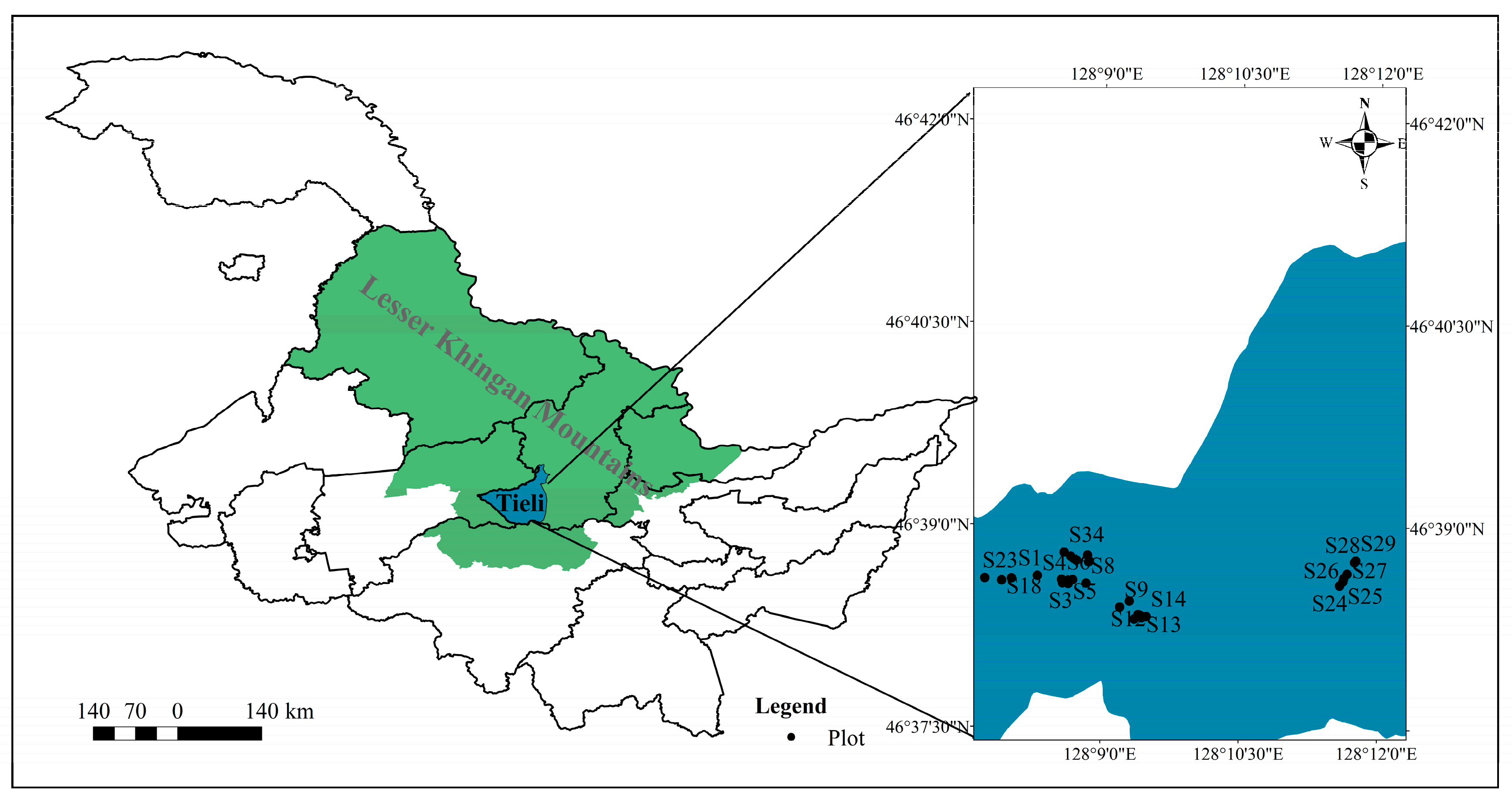
2.1. Study Site

The study area is situated in the northern part of Tieli, located in the central region of Heilongjiang Province (46°28′40″−47°27′30″ N, 127°38′20″−129°24′10″ E), adjacent to the Lesser Khingan Mountains and bounded by the Songnen Plain to the west. The Lesser Khingan Mountains serve as a significant forestry industry base in China, boasting abundant forest vegetation with a forest cover of 72.6%. The eastern section of Yanan Forest Farm falls within the Changbai flora zone, characterized by over 2000 plant species and undisturbed forests exhibiting dense tree growth and ground coverage both above and below the forest canopy. The climate exhibits a temperate monsoon pattern with an annual minimum air temperature reaching −38.8 °C and an annual maximum air temperature peaking at 31.6 °C. Additionally, it experiences an average annual effective cumulative air temperature of 2685.8 °C along with approximately 2367.6 h of sunlight per year. Throughout all seasons, there are notable day-to-night temperature fluctuations observed on a wide annual scale basis. Snowfall accumulates to an average thickness of 31 cm each year while precipitation amounts reach approximately 714.4 mm annually. The frost-free period spans about 152 days, primarily concentrated during June–August due to warm and rainy summers, which provide favorable conditions for short-term forest growth (Figure 1). This area boasts ample broadleaved tree species, including Quercus mongolica Fisch, Fraxinus mandshurica Rupr., Juglans mandshurica Maxim., Tilia tuan Szyszyl., Populus davidiana Dode., Acer pictum Thunb., Ulmus pumila L., and Betula platyphylla Sukaczev. These trees play a crucial role in maintaining ecological balance throughout China.

Study data were collected from 29 plots in mixed broadleaf forest surveyed at Yanan Forest Farm in 2023 (

Table 1. Basic characteristics of the studied plots.

Plot	Mean Elevation (m)	Slope (°)	Mean DBH (cm)	Density (Tree/ha)	Number of Species
S1	321	<5	20.31	725	6
S2	341	<5	17.51	700	9
S3	338	<5	21.85	533	5
S4	451	<5	17.45	733	8
S5	339	<5	24.08	541	6
S6	378	<5	21.12	542	6
S8	296	<5	21.01	600	11
S9	343	<5	17.64	825	8
S10	329	<5	22.83	450	8
S11	331	<5	18.38	758	7
S12	271	<5	18.72	625	6
S13	252	<5	20.18	741	10
S14	337	<5	12.39	1266	10
S17	305	<5	20.57	625	6
S18	296	5~15	22.92	508	6
S23	323	<5	11.89	1383	6
S24	325	<5	18.26	641	10
S25	345	<5	21.47	500	10
S26	352	<5	19.94	616	9
S27	346	<5	22.62	566	9
S28	356	<5	17.26	775	8
S29	357	15~20	15.34	741	14
S30	376	5~15	18.08	958	10
S31	370	15~25	16.78	1050	10
S32	352	<5	17.68	775	11
S33	360	<5	17.44	991	11
S34	367	<5	16.65	750	10
S35	354	<5	14.99	1050	7
S36	354	<5	17.8	708	9

). The neighborhood grid method was used to divide each plot of 0.12 hm² into 10 m × 10 m grids, and all trees with a diameter at breast height (DBH) ≥ 5 cm were recorded for tree species, number, diameter at breast height (DBH), tree height (H), crown width, condition, and coordinates.

2.2. Classifying Development Stages of Mixed Hard Broadleaf Forests

We selected the TWINSPAN two-way indicator species analysis method to classify the different DSs of stands. The TWINSPAN two-way indicator species analysis method is modified based on indicator species analysis, which can complete the classification of samples and species at the same time [26]. The two-way indicator species analysis of the species plot matrix (TWINSPAN) method divides all samples and species into two main categories, 0 and 1, and then divides each of these two main categories into two categories until the required level of division is reached. The five levels of pseudo-species chosen per species were 0–2, 2–5, 5–10, 10–20, and >20, using the R software TwinspanR package 0.2.2 [27].

Our data from 29 plots were collated to group Picea asperata, Abies fabri, Pinus koraiensis, and Larix gmelinii as conifers, and others as soft broadleaf. Thus, 11 tree species (groups) were used for indicator species: Fraxinus mandshurica, Juglans mandshurica, Phellodendron amurense, Acer pictum, Quercus mongolica Fisch, Tilia tuan, Ulmus pumila, Betula, Populus L., Conifers, and other soft broadleafs. They were grouped into volume percentages by species to form a matrix (Equation (1)).

$$Y=\left(\begin{array}{c}{B}_{1\times m}\\ V_{n\times m}\end{array}\right)$$

(1)

In the formula, $B_{1\times m}$ represent the 1$\times$m row vectors composed of tree species, $V_{n\times m}$ represents the n$\times$m matrix composed of tree species volume, and n, m represent the number of plots and species trees, respectively.

To make a reasonable assessment of the DSs in mixed hard broadleafs, we should not only consider the stand structural condition but also the changes in the stand growth. We selected eight stand factors, namely average diameter at breast height (D_g), average height (H_t), per hectare tree number (N), basal area (BA), volume (V), percentage of three precious hard broadleaf species (Fraxinus mandshurica, Juglans madshurica, Phellodendron amurensis) (Yk), and diameter distribution (q), to calculate tree species diversity (H₁) and size diversity(H₂). H₁ and H₂ were calculated as follows.

$$H_1=-{\displaystyle \sum _{i=1}^n{\displaystyle \frac{{BA}_i}{BA}}\mathit{ln}(}{\displaystyle \frac{{BA}_i}{BA}})$$

(2)

$$H_2=-{\displaystyle \sum _{i=1}^n{\displaystyle \frac{{BA}_j}{BA}}\mathit{ln}(}{\displaystyle \frac{{BA}_j}{BA}})$$

(3)

In the formula, BA_i and BA_j represent the basal area of the trees of species group i and diameter class j, respectively.

2.3. Stand Spatial Structure Optimization

2.3.1. SS Parameters Selection

We selected a 3 m buffer area to mitigate edge effects. This implies that trees within the core area were considered as reference trees, and their corresponding parameters were calculated, while other trees in the buffer area were regarded as neighbor trees. Six indices were used to analyze the SpS: M_c reflects stand species diversity by measuring the dissimilarity of species between the reference tree and its four nearest neighbors; W indicates the horizontal distribution pattern of both the reference tree and its four nearest neighbors; U represents the proportion of neighboring trees larger than the reference tree among all neighboring trees; S is used as an indicator to describe the vertical SpS of the forest, referring to forest vertical structure diversity, in which the stand layer index is in accordance with the International Union of Forestry Research Organization’s (IUFRO) standard for vertical stratification, which is based on the stand dominant height divided into three vertical layers, with a tree height less than or equal to 1/3 of the dominant height as the lower layer, between 1/3 and 2/3 dominant height as the middle layer, and greater than or equal to 2/3 dominant height as the upper layer; CI refers to the competitive status between the reference tree and its four nearest neighbors, which is based on diameter and distance; and K is a spatial indicator describing the level of light in a stand and is used to assess the adequacy of the space for individual tree growth [28,29,30] (

Table 2. SpS parameters and index definition.

Index	Formula	Definition
Complete mingling index (Mc)	$M_{c_i}={\displaystyle \frac{1}{2}}\left(D_i+{\displaystyle \frac{C_i}{n_i}}\right)·M_i$	Where $C_i$ is the number of different tree species in paired neighbours; $C_i/n_i$ is the degree of isolation of the nearest neighbour to the reference tree; $n_i$ is the number of nearest neighboring trees; $D_i$ is the Simpson index of the SpS unit i, $D_i=1-\sum _{j=1}^{S_i}{p}_j^2;$ $S_i$ is the tree species of the SpS unit I; $p_j$ is the proportion of trees of the jth species; $M_i$ is a simple mingling index, $M_i={\displaystyle \frac{1}{n}}\sum _{j=1}^n{v}_{ij}$, where $v_{ij}=0$, if reference tree i and its neighbor tree j are the same white tree species, otherwise, $v_{ij}=1$
Uniform angle index (W)	$W_i={\displaystyle \frac{1}{n}}{\displaystyle \sum _{j=1}^n}{w}_{ij}$	Where $w_{ij}=\left\{\begin{array}{c}1;\mathit{if }{\alpha }_j<{\alpha }_0={72}^{°}\\ 0;\mathit{otherwise}\end{array}\right\}$; and α is the angle between two adjacent trees
Dominance index (U)	$U_i={\displaystyle \frac{1}{n}}{\displaystyle \sum _{j=1}^n}{z}_{ij}$	where zij takes the value 1 if the jth neighbor (dj) is smaller than the reference tree i(di), and the value 0, otherwise, $z_{ij}=\left\{\begin{array}{c}1;d_j<d_i\end{array}\right\}$
Stand layer index (S)	$S_i={\displaystyle \frac{1}{n}}{\displaystyle \sum _{j=1}^n}{S}_{ij}$	where Sij = 0, indicating that the neighbour tree and the reference tree are not in the same vertical layer; otherwise, Sij = 1
Hegyi competition index (CI)	${CI}_i={\displaystyle \sum _{i=1}^{n_i}}{\displaystyle \frac{d_j}{d_i·L_{ij}}}$	where di is the diameter of the reference tree, dj is the diameter of the neighbouring trees, and Lij is the Euclidean distance between them
Open degree (K)	$K_i={\displaystyle \frac{1}{n}}{\displaystyle \sum _{j=1}^{n_i}}{\displaystyle \frac{D_{ij}}{H_{ij}}}$	where Hj is the height of the neighboring tree j, and Dij is the distance between them

).

2.3.2. SpS Optimization Model

The horizontal distribution, competition between trees, and tree height and growth space can be characterized using $M_c$, W, U, S, CI, and K. The quantitative SpS indices mentioned above can be quickly assessed and have clear biological significance. The determination of the optimal trees for harvesting can be achieved by evaluating the relationship between each reference tree and its four nearest reference trees [31]. However, it should be noted that these indices exhibit significant variations in both magnitude and measuring units. Thus, in this study, the SpS optimization model Q(x) was proposed based on the multi-objective programming method. The maximum value Q(x) indicates that the optimal SpS is closer to the natural and ideal spatial distribution; it shows that the tree species have the maximum mixing degree, minimal competition between trees, more adequate light conditions and space for tree growth, and the most stand vertical structure diversity.

The model is as follows:

$$Q\left(x\right)={\displaystyle \frac{\frac{1+Mc\left(x\right)}{{\sigma }_{M_c}}·\frac{1+S\left(x\right)}{{\sigma }_S}.\frac{1+K\left(x\right)}{{\sigma }_K}}{\left[1+CI\left(x\right)·{\sigma }_C\right]·\left[1+U\left(x\right)·{\sigma }_U\right]·\left[1+\left|W\left(x\right)-0.475\right|+\left|W\left(x\right)-0.517\right|\right]·{\sigma }_W}}$$

(4)

$$N=N_0$$

(5)

$$D=D_0$$

(6)

$$1.2\le q\le 1.7$$

(7)

$$M_c\ge M_{c0}$$

(8)

$$0.475\le W\le 0.517$$

(9)

$$U\le U_0$$

(10)

$$S\ge S_0$$

(11)

$$CI\le {CI}_0$$

(12)

$$K\ge K_0$$

(13)

where the q-value is a measure of diameter distribution commonly used in forest inventory management in the northeast of China, where a negative exponential function is used to fit the relationship between tree number and diameter class with the expression q = exp(a∙d), where a is the estimated parameter and d is the diameter class. The q-value of natural heterogeneous forests varies between 1.2 and 1.7, which is a reasonable range for transformation [32,33]. N and N₀ are the numbers of diameter classes before and after optimization, and D and D₀ are the tree species before and after optimization, respectively. $M_{c0}, U_0, S_0, {CI}_0, K_0, M_c, U, S, CI, K$ are the values of the complete mixing index, dominance index, stand layer index, Hegyi competition index, and open degree before and after optimization, respectively. W is the uniform angle index; when the distribution pattern of the trees is random, the W values range from 0.475 to 0.517 [34]. ${\sigma }_{M_c}, {\sigma }_U, {\sigma }_w, {\sigma }_S, {\sigma }_{CI},$ and ${\sigma }_K$ are the standard deviations of the complete mixing index, uniform angle index, dominance index, stand layer index, Hegyi competition index, and open degree.

Equation (4) is the objective function for optimizing SpS. As the q-value increases, the existing SS approaches the optimum SS. Equation (5) is diameter distribution constraint. Equation (6) is the tree species constraint. Equation (7) is the q-value constraint which controls the optimized stand q-values between 1.2 and 1.7. Equations (8)–(13) are the SpS constraints.

2.3.3. Optimization Simulation

In this study, we selected 3 plots (S31, S23, and S28) at different DSs (forest establishment stage, competitive growth stage, and quality selection stage), respectively, to optimize the stand SpS. Since the model contains a large number of integer variables, solving it by the exhaustive method takes a lot of time. Therefore, it is acceptable to use the Monte Carlo algorithm for the simulation of interlopes to obtain a suboptimal solution to the problem [35]. The Monte Carlo algorithm is based on the principle of random sampling. It uses a random number function provided to perform a fast random sampling of feasible points in the constrained optimization problem.

Therefore, the tree removal intensity is set to 10%, 20%, and 30%, and the initial number of simulations is set to 5000. All objective function values that satisfy the constraints are defined as valid simulations, and the simulation with the largest objective function value is identified among these simulations. We consider this thinning simulation to be an approximate solution to the optimal solution of this problem.

3. Results

3.1. Classifying Development Stages of Mixed Hard Broadleaf Forests

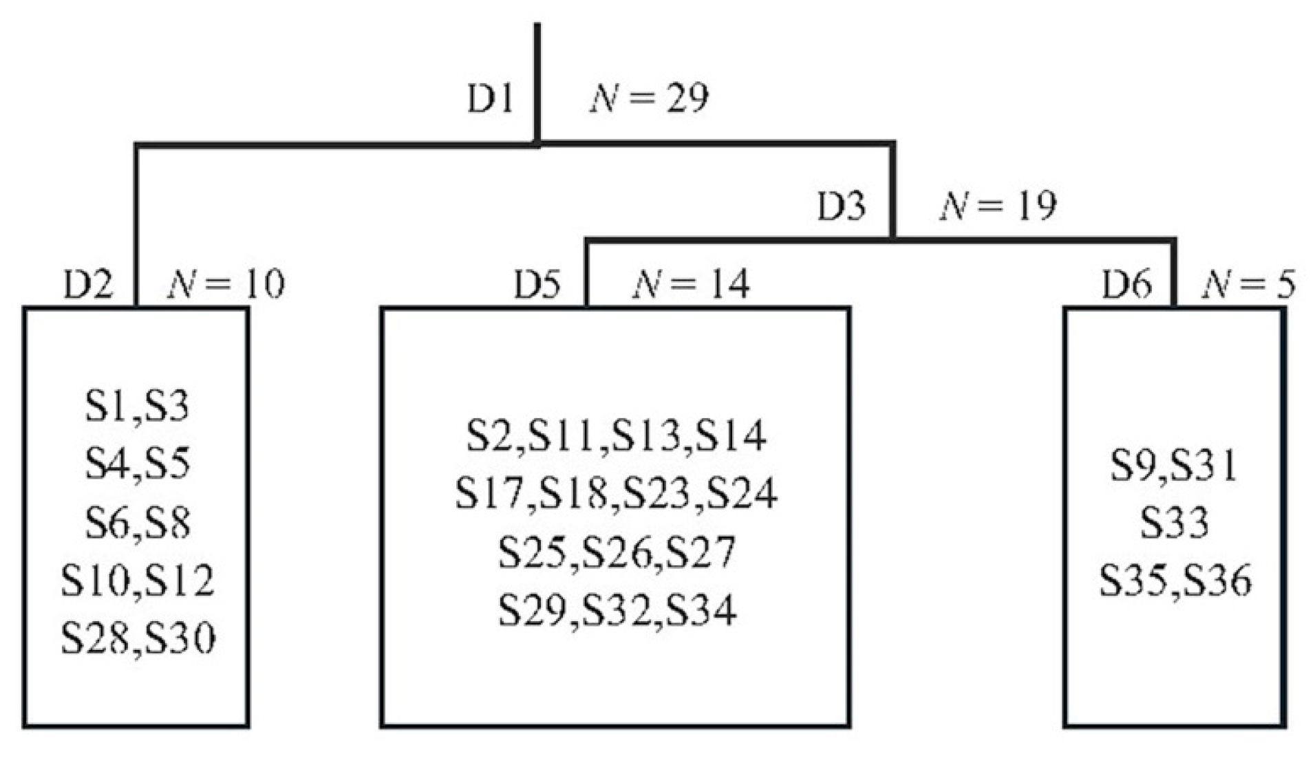
3.1.1. Twinspan Classification Results

Figure 2 shows the 29 plots of the TWINSPAN classification process and their results. The 29 mixed broadleaf plots were divided into three categories by two divisions. With the exclusion of the misclassified plots and the combination of the information on the species composition of the plots, the stand characteristics of each class were as follows: there were 10 plots accounting for 34.5% in Type I, and the main tree species are Fraxinus mandshurica, Juglans madshurica, and Phellodendron amurensis, with volume composition ratios of 24.9%, 32.4%, and 15.6%, respectively; there were 14 plots accounting for 48.3% in Type II, where the main tree species are Juglans madshurica, Ulmus pumila, and Fraxinus mandshurica with volume composition ratios of 26.8%, 22.8%, and 16.1%, respectively; there were 5 plots accounting for 17.2% in Type III, where the main tree species are Fraxinus mandshurica, Juglans madshurica, Phellodendron amurensis, and Ulmus pumila with a total volume composition of 47.1%, in which the three precious hard broadleaf species (Fraxinus mandshurica, Juglans madshurica, Phellodendron amurensis) accounted for 29.9%, and Ulmus pumila accounted for 17.2%.

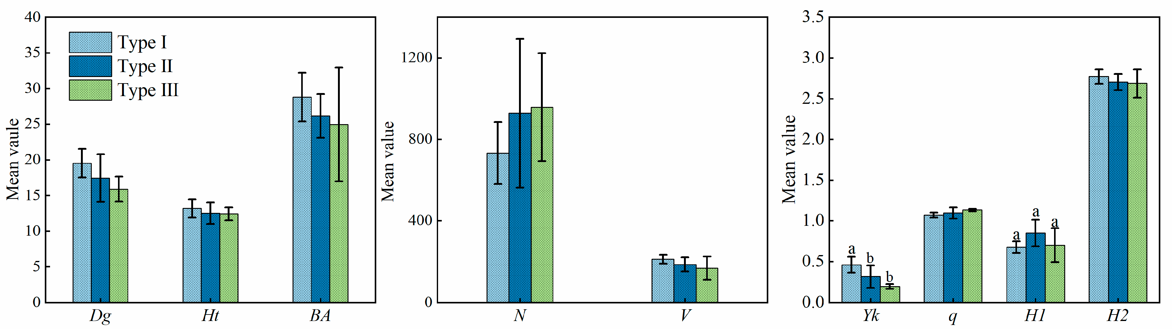
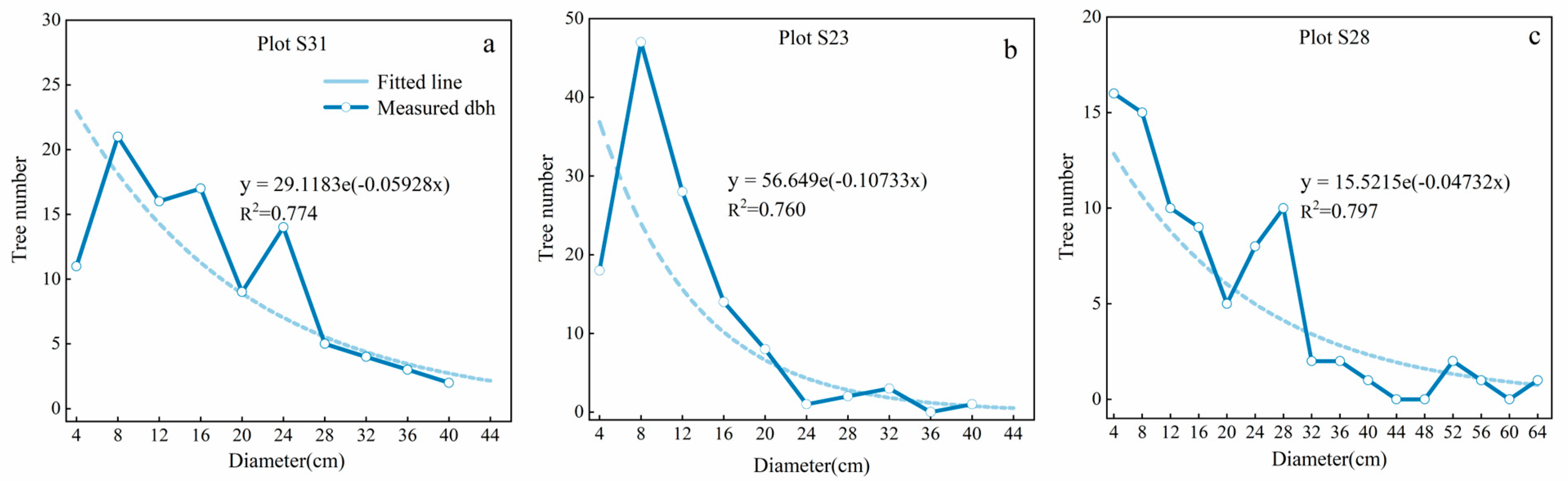
3.1.2. Stand Growth Analysis for TWINSPAN Classification

Figure 3 shows the 29 plots’ stand growth index change for TWINSPAN classification, where dbh, H_t, base area, number, v, q, H₁ and H₂ were not significant in different classifications. YK was significant in different classifications (p < 0.05); the dbh, H_t, base area, v, and YK values are sorted by Type I > Type II > Type III. The number and q values are sorted by Type I < Type II < Type III; Type II has the greatest tree species diversity (H₁) and the least size diversity (H₂), and Type III has the greatest size diversity (H₂) and the least tree species diversity (H₁). Therefore, Type III is in the early stage of development and Type I is in the late stage of development. As the stand grows and develops, the pioneer tree species gradually decline and tree species diversity (H₁) decreases, and tree size richness increases. Taking a comprehensive view of the tree species composition, SS, and growth, our study classified the DSs of 29 mixed hard broadleaf plots by Type III (forest establishment stage)—Type II (competitive growth stage)—Type I (quality selection stage).

3.2. Stand Spatial Structure Optimization

Figure 4 shows the distribution of the number of plants in diameter steps at different growth and development stages. At the forest quality selection stage, the diameter distribution was the widest distribution, which was between 4 and 64 cm (S28). In S31 and S23, the diameter range was 4–40 cm, with obvious differences in diameter class distribution. Plot S31 and Plot S28 had 64% and 61% of the number of the total trees in the 4–16 diameter classes, respectively; Plot S23 had the largest number of trees in the 4–16 diameter classes, with 87% of the total number. In all three phases, the number of 4–24 cm diameter trees accounted for 95%, and the number of large-diameter trees accounted for about 2% of the total number.

In Plot S31, 8–24 cm trees were abundant, forming an asymmetric, left-sloping, multi-peaked curve. After the last peak in the 24 cm diameter class, the number of trees started to decrease with increasing diameter classes; Plot S23 showed that the diameter distribution of the unevenly aged stands is characterized by a single-peak inverted ‘J’ curve that peaks at an 8 cm diameter, it indicated that there were a lot of young trees and seedlings, and it could be continuously recruited, while large-diameter trees were few and had many deficiencies; in general, the number of trees in the stand decreased sharply as the diameter class increased from 6 cm upwards. Plot S28 was a multi-peaked mountainous curve with peaks at 8 cm and 28 cm, in which the middle- and small-diameter classes had more trees and large-diameter classes had fewer trees. When the diameter class was 20–28 cm, the number of trees increased, and the number of 8–20 cm and 28 cm trees decreased. When analyzed with the q-value, Plot S31 (1.267) had a slightly lower q-value than Plot S23 (1.536) and Plot S28 (1.227); however, Plot S28 was better fitted to the diameter of InN (R² = 0.797) than Plot S31 (R² = 0.774) and Plot S23 (R² = 0.760).

Table 3. The different SS-optimized variables for the three plots.

Plot	Intensity	Number (Tree)	Mc	S	CI	W	U	q	Q(x)	RIP
S31	0%	126	0.601	0.573	2.610	0.526	0.497	1.267	178.425
	10%	12	0.661	0.603	2.220	0.516	0.500	1.260	607.397	124.04
	20%	24	0.685	0.631	2.124	0.497	0.500	1.208	677.869	11.60
	30%	36	0.667	0.618	1.946	0.503	0.506	1.339	733.350	8.18
S23	0%	166	0.400	0.386	3.043	0.523	0.486	1.536	57.312
	10%	16	0.439	0.556	2.275	0.500	0.479	1.500	248.586	333.74
	20%	32	0.455	0.530	2.042	0.510	0.474	1.507	395.122	58.94
	30%	48	0.503	0.540	1.823	0.491	0.479	1.449	530.569	34.27
S28	0%	92	0.455	0.486	2.372	0.533	0.515	1.227	172.444
	10%	10	0.469	0.593	2.096	0.513	0.513	1.212	373.914	116.83
	20%	20	0.465	0.598	1.969	0.511	0.511	1.228	407.176	8.89
	30%	30	0.470	0.560	1.972	0.5000	0.495	1.200	309.324	−24.03

shows that there is a certain difference in SS index optimization before and after different DS stands. It shows the statistical features of different spatial parameters for three different DS stands with 0%, 10%, 20%, and 30% of trees removed, respectively. The M_c value of the S23 plot is 0.400, which belongs to the medium mixing degree, the M_c value of the S28 plot is 0.455, which belongs to the medium mixing degree, and the M_c value of the S31 plot is greater than 0.5, which belongs to the strong mixing degree, greater than the S23 and S28 plots.

The average U value of Plots S23, S28, and S31 are 0.484, 0.497, and 0.515, respectively, indicating that the stands are in homogeneous condition. The average W value of the different DS stands ranges from 0.523 to 0.533, which is greater than 0.517, indicating that the stands all have significant agglomeration distribution patterns. The average S values of Plots S23, S28, and S31 are 0.368, 0.468, and 0.573, respectively, indicating that Plot S31 has the highest vertical structural diversity. The average CI value (3.043) of Plot S23 reflects that its tree competition pressure is higher than that of Plots S31 (2.372) and S28 (2.610). The q-value of Plots S23, S28, and S31 are 1.536, 1.227, and 1.267, respectively, which are all significantly within the range of 1.2 and 1.7. The Q(x) index is also a logical negative index; the Q(x) values for plots S23, S28, and S31 are 57.312, 172.444, and 178.425, respectively; therefore, the lowest Q(x) value was found in Plot S23.

Table 3 shows the changes in different DS stand structure indices with the increase in thinning intensity. When thinning intensity increases by 1%, the M_c, S, CI, W, U, and q in Plot S31 all increase, respectively; 0.099, 0.0523, 0.1756, 0.0193, 0.006, 0.0055. The trend of the increase or decrease in the SpS index before and after optimization is the same at different stages of the stands, but the magnitude of change is different. With the increase in thinning intensity, the spatial indices of M_c and S increased significantly, while CI decreased. The value of Q(x) of the stand spatial structure optimization function in different stages increased with the increase in cutting intensity, and Q(x) increased by 124.04, 11.60, and 8.18 for the S31 plot, respectively. The Q(x) value increased with the optimized thinning intensity, which is equivalent to that when the thinning intensity increased by 1%, and the Q(x) of the stand after different DS optimizations increased by 124.04%, 333.74%, and 116.83%, respectively. This result also shows that the relative increase ratio (RIP) of the optimization function Q(x) between any two consecutive thinning intensifications decreases significantly as the selective thinning intensification increases, suggesting that the removal of 10% of trees may be the optimal intensity from the perspective of optimizing the forest SpS in all three plots.

For mixed hard broadleaf forests, the harvest possibilities of the three precious hard broadleaf species (Fraxinus mandshurica, Juglans madshurica, Phellodendron amurensis) were significantly higher than those of other species, and higher than in species when removing 30% of the trees, and more than twice as high as species when 10% of the trees were removed. The harvest of Ulmus pumila accounted for approximately 7.4%, Tilia tuan for approximately 14.2%, Acer pictum Thunb. for approximately 6.7%, and Fraxinus mandshuric for approximately 7.6% of the lower harvesting intensity in Plot S31; Figure 5, Figure 6 and Figure 7 show the spatial distribution patterns of trees cut after the spatial optimization of different DS stands when the optimal cutting intensity is 10%, in which SpS is improved, reducing the competitive pressure among trees, adjusting the distribution pattern of trees, and providing space for tree growth.

4. Discussion

Stand growth and DSs reflect natural and anthropogenic disturbances, and stands are usually located in each stage based on characteristics such as stand age, structure, and function. Their growth and DS are identified by the vertical and horizontal structure of the stand, canopy gaps, volume, number of dead trees, regeneration, and species composition of the stand [2,36]. Depending on habitat and site conditions, SS and the length of developmental stages vary considerably. Typically, forests have three main important developmental stages, including the primary stage (regeneration and growth), the optimum stage (maturity and senescence), and the decay stage (decomposition); each growth and development stage has processes and characteristics that create specific conditions for species response and the number of standing trees at different growth stages [3,37]. Stand types, tree ages, and stand densities vary, affecting changes in forest growth, biodiversity, soil fertility, soil nutrient levels, and plant nutrient uptake, which in turn affect forest productivity, diversity, and stability [38,39].

We selected the TWINSPAN two-way indicator species analysis method to classify the different DSs of stands. The obtained results indicated that by taking a comprehensive analysis of the tree species composition, SS, and growth through eight stand indicators (average diameter at breast height (D_g), average height (H_t), per hectare tree number(N), basal area (BA), volume (V), percentage of three precious hard broadleaf species (Fraxinus mandshurica, Juglans madshurica, Phellodendron amurensis) (Yk)), along with tree species diversity (H₁) and size diversity(H₂), our study classified the DSs of 29 mixed hard broadleaf plots by Type III (forest establishment stage)—Type II (competitive growth stage)—Type I (quality selection stage). In the process of forest growth and development, the pioneer species first occupied the main forest layer, and with the development of community succession, the pioneer species gradually declined and decreased, and the companion species invaded and then gradually occupied the main forest layer in the later stage of top pole species [40]. The broadleaved Korean pine forest is a typical horizontal zonal overstory community in the Lesser Khingan Mountains, in which the coniferous species are dominated by Korean pine, and some of the coniferous species, such as Picea jezoensis, Picea koraiensis Nakai, and Abies nephrolepis, etc., are accompanied by coniferous species, and the broadleaved species are mainly Tilia amurensis, Acer pictum Thunb., Quercus mongolica Fisch, Betula costata Trautv., Ulmus pumila, and three precious hard broadleaf species (Fraxinus mandshurica, Juglans madshurica, Phellodendron amurensis); due to differences in soil conditions, the succession process of secondary forests resulting from the disturbance of the broadleaved Korean pine forest will vary [41,42]. In the absence of the Korean pine seed source, the trees in the community will die and regenerate over many generations, and the succession will converge in the intermediate community consisting of coniferous, hard broadleaved, and soft broadleaved mixed forests composed of different species [43]. The intermediate stages in the development of community succession are the three stages of growth and development in this study.

Stand structure characteristics play an important factor in forest management optimization and evaluation, reflecting the tree’s growth and basic characteristics in the stand. Different species compositions, diameter class distribution tree distribution patterns, and arrangements lead to different structural characteristics of DS stands [44,45]. SS is usually described in two directions, horizontal and vertical structure. Differences in the horizontal and vertical structure of different stands have implications for tree and understory plant growth, regeneration, biodiversity, stand ecological function, and wildlife habitat [46,47]. Therefore, how can we adjust the rationality and diversity of SSs through the stand optimization function, especially in the optimization of different DSs [23,48,49]? This study presented an SpS optimization model, which was applied to three mixed hard broadleaf stands of different DSs. Since the three plots were extracted from different DSs, there were obvious differences between their spatial and nonspatial structural characteristics. Differences between the three plots were also evident in the number of tree species and the distribution of diameter classes, which are traditional indicators of forest structure.

The Q(x) value all increased and could effectively improve the SpS significantly. The Q(x) increased by 124.01%, 333.74%, 116.83% compared with those with no harvest, the RIP decreased with the increase in thinning intensity in stands at different DSs. By comparing different optimal cutting intensities, it was found that the RIP value is the largest when the optimal cutting intensity is 10%. This means that improving SS characteristics is most effective when the optimization intensity is low at 10%. The State Forestry Bureau of China’s forest management policies and regulations also coincide with this intensity [50]. Low-intensity harvest is the best optimization intensity from the perspective of SS optimization, though optimal harvesting intensity varies with the different optimization objectives (carbon sequestration and stocks, soil physical and chemical properties) [51,52].

The allocated harvest within this intensity was mainly focused on the trees with high competition, low health, and clumped distribution, while only a handful of trees were harvested to adjust to neighborhood-based structures (Figure 5, Figure 6 and Figure 7). In SBFM management, the maximum thinning intensity is selected by considering the relationship between the central and adjacent trees in the structural unit, so as to adjust spatial distribution and species diversity [53,54]. Overall, the stand structure parameters were optimized by comparison. This optimized the post-stand mingling degree, increasing the uniform angle index, reduced competitive pressure among trees, and decreased densities. The change in the spatial distribution pattern of the stand can increase the light conditions, reduce the competition between neighboring trees, and promote the growth of regenerated trees.

5. Conclusions

We propose that the TWINSPAN two-way indicator species combination with stand growth indicators can more accurately classify the DS of mixed hard broadleaf forests. Meanwhile, we propose a stand SpS optimization model for three elected plots. Optimizing the SpS improved the Q(x) by 124.04%, 333.74%, and 116.83%, and when the RIP reached the maximum value, it indicated that the cutting intensity was at the optimal intensity, and 10% is the optimal cutting intensity in this study. Moreover, this optimization model can be applied to the optimal management of stands at different stages to guide the optimization of natural forest structures under different growth and DSs.

References

1. Král, K.; McMahon, S.M.; Janík, D.; Adam, D.; Vrška, T. Patch mosaic of developmental stages in central European natural forests along vegetation gradient. For. Ecol. Manag. 2014, 330, 17–28. [Google Scholar] [CrossRef]
2. Gong, Z.; Kang, X.; Gu, L. Quantitative division of succession and spatial patterns among different stand developmental stages in Changbai Mountains. J. Mt. Sci. 2019, 16, 2063–2078. [Google Scholar] [CrossRef]
3. Dai, L.; Qi, L.; Wang, Q. Changes in forest structure and composition on Changbai Mountain in Northeast China. Ann. For. Sci. 2011, 68, 889–897. [Google Scholar] [CrossRef]
4. Collins, R.J.; Carson, W.P. The effects of environment and life stage on Quercus abundance in the eastern deciduous forest, USA: Are sapling densities most responsive to environmental gradients? For. Ecol. Manag. 2004, 201, 241–258. [Google Scholar] [CrossRef]
5. Hao, Z.; Zhang, J.; Song, B.; Ye, J.; Li, B. Vertical structure and spatial associations of dominant tree species in an old-growth temperate forest. For. Ecol. Manag. 2007, 252, 1–11. [Google Scholar] [CrossRef]
6. Král, K.; Vrška, T.; Hort, L.; Adam, D.; Šamonil, P. Developmental phases in a temperate natural spruce-fir-beech forest: Determination by a supervised classification method. Eur. J. For. Res. 2009, 129, 339–351. [Google Scholar] [CrossRef]
7. Glatthorn, J.; Feldmann, E.; Tabaku, V.; Leuschner, C.; Meyer, P. Classifying development stages of primeval European beech forests: Is clustering a useful tool? BMC Ecol. 2018, 18, 47. [Google Scholar] [CrossRef]
8. Huber, M.O. Statistical models to identify stand development stages by means of stand characteristics. Can. J. For. Res. 2011, 41, 111–123. [Google Scholar] [CrossRef]
9. Uhl, C.; Buschbacher, R.; Serrao, E.A.S. Abandoned Pastures in Eastern Amazonia. I. Patterns of Plant Succession. J. Ecol. 1988, 76, 663. [Google Scholar] [CrossRef]
10. Leibundgut, H. Uber Zweck und Methodik der Strukturund Zuwachsanalyse von Urw€aldern. Schweiz. Z. Forstwes. 1959, 110, 111–124. [Google Scholar]
11. Leibundgut, H. Uber die Dynamik europaischer Urwalder. Allg. Forst Z. 1978, 33, 686–690. [Google Scholar]
12. Goodell, L.; Faber-Langendoen, D. Development of stand structural stage indices to characterize forest condition in Upstate New York. For. Ecol. Manag. 2007, 249, 158–170. [Google Scholar] [CrossRef]
13. Podlaski, R. Suitability of the selected statistical distributions for fitting diameter data in distinguished development stages and phases of near-natural mixed forests in the Świętokrzyski National Park (Poland). For. Ecol. Manag. 2006, 236, 393–402. [Google Scholar] [CrossRef]
14. Zenner, E.K.; Peck, J.E.; Hobi, M.L.; Commarmot, B. Validation of a classification protocol: Meeting the prospect requirement and ensuring distinctiveness when assigning forest development phases. Appl. Veg. Sci. 2016, 19, 541–552. [Google Scholar] [CrossRef]
15. Feldmann, E.; Glatthorn, J.; Hauck, M.; Leuschner, C. A novel empirical approach for determining the extension of forest development stages in temperate old-growth forests. Eur. J. For. Res. 2018, 137, 321–335. [Google Scholar] [CrossRef]
16. Gao, T.; Hedblom, M.; Emilsson, T.; Nielsen, A.B. The role of forest stand structure as biodiversity indicator. For. Ecol. Manag. 2014, 330, 82–93. [Google Scholar] [CrossRef]
17. Ali, A. Forest stand structure and functioning: Current knowledge and future challenges. Ecol. Indic. 2019, 98, 665–677. [Google Scholar] [CrossRef]
18. Baran, J.; Pielech, R.; Kauzal, P.; Kukla, W.; Bodziarczyk, J. Influence of forest management on stand structure in ravine forests. For. Ecol. Manag. 2020, 463, 118018. [Google Scholar] [CrossRef]
19. Hui, G.; Zhang, G.; Zhao, Z.; Yang, A. Methods of Forest Structure Research: A Review. Curr. For. Rep. 2019, 5, 142–154. [Google Scholar] [CrossRef]
20. Aguirre, O.; Hui, G.; von Gadow, K.; Jiménez, J. An analysis of spatial forest structure using neighbourhood-based variables. For. Ecol. Manag. 2003, 183, 137–145. [Google Scholar] [CrossRef]
21. Gadow, K.V.; Zhang, C.Y.; Wehenkel, C.; Pommerening, A.; Corral-Rivas, J.; Korol, M.; Myklush, S.; Hui, G.Y.; Kiviste, A.; Zhao, X.H. Forest Structure and Diversity. In Continuous Cover Forestry; Springer: Dordrecht, The Netherlands, 2011; pp. 29–83. [Google Scholar] [CrossRef]
22. Pastorella, F.; Paletto, A. Stand structure indices as tools to support forest management: An application in Trentino forests (Italy). J. For. Sci. 2013, 59, 159–168. [Google Scholar] [CrossRef]
23. Ye, S.; Zheng, Z.; Diao, Z.; Ding, G.; Bao, Y.; Liu, Y.; Gao, G. Effects of Thinning on the Spatial Structure of Larix principis-rupprechtii Plantation. Sustainability 2018, 10, 1250. [Google Scholar] [CrossRef]
24. Lopes, J.F.B.; Lopes, F.B.; Araújo, I.C.D.S.; Pereira, E.C.B.; Brandão, M.L.S.M.; Feitosa, E.D.O.; Luna, N.R.D.S.; Sousa, G.G.D.; Amorim, A.V.; Iwata, B.D.F.; et al. How Forest Management with Clear-Cutting Affects the Regeneration, Diversity and Structure of a Seasonally Dry Tropical Forest in Brazil. Forests 2023, 14, 1870. [Google Scholar] [CrossRef]
25. Dittrich, S.; Hauck, M.; Jacob, M.; Rommerskirchen, A.; Leuschner, C. Response of ground vegetation and epiphyte diversity to natural age dynamics in a Central European Mountain spruce forest. J. Veg. Sci. 2012, 24, 675–687. [Google Scholar] [CrossRef]
26. Hill, M.O. TWINSPAN: A fortran program of arranging multivariate data in an ordered two way table by classification of individual and attributes. In Section of Ecology and Systematics; Cornell University: Ithaca, NY, USA, 1979. [Google Scholar]
27. Roleček, J.; Tichý, L.; Zelený, D.; Chytrý, M. Modified TWINSPAN classification in which the hierarchy respects cluster heterogeneity. J. Veg. Sci. 2009, 20, 596–602. [Google Scholar] [CrossRef]
28. Hu, Y.; Bo, H.Y.; Bo, X.H. Structured Forest Management; China Forestry Publishing: Beijing, China, 2007; pp. 56–60. ISBN 9787503847639. [Google Scholar]
29. Li, Y.; Hui, G.; Zhao, Z.; Hu, Y. The bivariate distribution characteristics of spatial structure in natural Korean pine broad-leaved forest. J. Veg. Sci. 2012, 23, 1180–1190. [Google Scholar] [CrossRef]
30. Hui, G.Y.; Von Gadow, K.; Hu, Y.B.; Chen, B.W. Characterizing Forest spatial distribution pattern with the mean value of uniform angle index. Acta Ecol. Sin. 2004, 24, 1225–1229. (In Chinese) [Google Scholar]
31. Pukkala, T.; Ketonen, T.; Pykäläinen, J. Predicting timber harvests from private forests—A utility maximisation approach. For. Policy Econ. 2003, 5, 285–296. [Google Scholar] [CrossRef]
32. Schwartz, J.W.; Nagel, L.M.; Webster, C.R. Effects of uneven-aged management on diameter distribution and species composition of northern hardwoods in Upper Michigan. For. Ecol. Manag. 2005, 211, 356–370. [Google Scholar] [CrossRef]
33. Gadow, K.V.; Hui, G. Modelling Forest Development; Forestry Sciences Series; Springer: Dordrecht, The Netherlands, 1999. [Google Scholar] [CrossRef]
34. Hui, G.Y.; Hu, Y.B.; Liu, R.H. Methods of Analyzing Stand Spatial Dominance in Forest Observational Studies. Res. Inst. For. 2019, 2, 12. (In Chinese) [Google Scholar]
35. Neto, T.; Constantino, M.; Martins, I.; Pedroso, J.P. A multi-objective Monte Carlo tree search for forest harvest scheduling. Eur. J. Oper. Res. 2020, 282, 1115–1126. [Google Scholar] [CrossRef]
36. Gu, L.; O’Hara, K.L.; Li, W.; Gong, Z. Spatial patterns and interspecific associations among trees at different stand development stages in the natural secondary forests on the Loess Plateau, China. Ecol. Evol. 2019, 9, 6410–6421. [Google Scholar] [CrossRef] [PubMed]
37. Gokturk, A.; Tiras, H. Stand structure and spatial distribution of trees at different developmental stages and stand layers in mixed stands in Artvin region, Turkey. Appl. Ecol. Environ. Res. 2020, 18, 6163–6179. [Google Scholar] [CrossRef]
38. Zhang, M.; Kang, X.; Meng, J.; Zhang, L. Distribution patterns and associations of dominant tree species in a mixed coniferous-broadleaf forest in the Changbai Mountains. J. Mt. Sci. 2015, 12, 659–670. [Google Scholar] [CrossRef]
39. Petritan, I.C.; Marzano, R.; Petritan, A.M.; Lingua, E. Overstory succession in a mixed Quercus petraeaFagus sylvatica old growth forest revealed through the spatial pattern of competition and mortality. For. Ecol. Manag. 2014, 326, 9–17. [Google Scholar] [CrossRef]
40. Christensen, N.L.; Peet, R.K. Convergence During Secondary Forest Succession. J. Ecol. 1984, 72, 25. [Google Scholar] [CrossRef]
41. Zhou, C.F.; Zhang, H.R.; Lu, J.; Zhang, X.H. Disturbances and Succession Laws of Main Natural Secondary Forests in Northeast China. For. Res. 2021, 34, 175–183. [Google Scholar] [CrossRef]
42. Zhou, Y.L.; Zhao, G.Y. Types, distribution and succession patterns of natural secondary forests Lesser Khingan Mountains—Changbai Mountain forest area. J. Northeast. For. Univ. 1964, 33–45. (In Chinese) [Google Scholar]
43. Lu, L.L. Study on Community Structure Characteristics of Different Succession Stages of Broad-leaved Korean Pine Forest in Changbai Mountain. Ph.D. Thesis, BeiHua University, Changchun, China, 2019. [Google Scholar]
44. Drössler, L.; Feldmann, E.; Glatthorn, J.; Annighöfer, P.; Kucbel, S.; Tabaku, V. What Happens after the Gap?—Size Distributions of Patches with Homogeneously Sized Trees in Natural and Managed Beech Forests in Europe. Open J. For. 2016, 6, 177–190. [Google Scholar] [CrossRef]
45. McElhinny, C.; Gibbons, P.; Brack, C.; Bauhus, J. Forest and woodland stand structural complexity: Its definition and measurement. For. Ecol. Manag. 2005, 218, 1–24. [Google Scholar] [CrossRef]
46. Wang, H.X.; Huang, S.X.; Zhang, S.S.; Peng, H.; Cao, K.F. Localized neighborhood species mingling is correlated with individual tree size inequality in natural forests in South China. Ann. For. Sci. 2021, 78, 102. [Google Scholar] [CrossRef]
47. Wang, Y.; Li, J.; Cao, X.; Liu, Z.; Lv, Y. The Multivariate Distribution of Stand Spatial Structure and Tree Size Indices Using Neighborhood-Based Variables in Coniferous and Broad Mixed Forest. Forests 2023, 14, 2228. [Google Scholar] [CrossRef]
48. Li, Y.; Hui, G.; Wang, H.; Zhang, G.; Ye, S. Selection priority for harvested trees according to stand structural indices. iFor.-Biogeosci. For. 2017, 10, 561–566. [Google Scholar] [CrossRef]
49. Li, Y.; Ye, S.; Hui, G.; Hu, Y.; Zhao, Z. Spatial structure of timber harvested according to structure-based forest management. For. Ecol. Manag. 2014, 322, 106–116. [Google Scholar] [CrossRef]
50. State Forestry Bureau. Regulations for Forest Tending; China Standards Press: Beijing, China, 2015. (In Chinese) [Google Scholar]
51. Dong, L.; Wei, H.; Liu, Z. Optimizing Forest Spatial Structure with Neighborhood-Based Indices: Four Case Studies from Northeast China. Forests 2020, 11, 413. [Google Scholar] [CrossRef]
52. Qiu, H.; Zhang, H.; Lei, K.; Hu, X.; Yang, T.; Jiang, X. A New Tree-Level Multi-Objective Forest Harvest Model (MO-PSO): Integrating Neighborhood Indices and PSO Algorithm to Improve the Optimization Effect of Spatial Structure. Forests 2023, 14, 441. [Google Scholar] [CrossRef]
53. Dong, L.; Bettinger, P.; Liu, Z. Optimizing neighborhood-based stand spatial structure: Four cases of boreal forests. For. Ecol. Manag. 2022, 506, 119965. [Google Scholar] [CrossRef]
54. Liu, H.; Dong, X.; Meng, Y.; Gao, T.; Mao, L.; Gao, R. A novel model to evaluate spatial structure in thinned conifer-broadleaved mixed natural forests. J. For. Res. 2023, 34, 1881–1898. [Google Scholar] [CrossRef]
Figure 1. The locations of the studied forest in the Lesser Khingan Mountains in northeastern China and the distribution of the studied plots in the Yanan Forest Farm.
Forests 15 01653 g001
Figure 2. Plot TWINSPAN classification results.
Forests 15 01653 g002
Figure 3. The stand factors of mixed hard broadleaf forest DS classification. (a b indicates level of significance in different classifications).
Forests 15 01653 g003
Figure 4. Diameter classes of the three plots from different DSs. ((ac) represent Plot S31, Plot S23 and Plot S28).
Forests 15 01653 g004
Figure 5. When the cutting intensity is 10%, the colors of the circles in Plot S31 indicate different tree species. × red indicates the distribution pattern of optimized harvested trees.
Forests 15 01653 g005
Figure 6. When the cutting intensity is 10%, the colors of the circles in Plot S23 indicate different tree species. × red indicates the distribution pattern of optimized harvested trees.
Forests 15 01653 g006
Figure 7. When the cutting intensity is 10%, the colors of the circles in Plot S28 indicate different tree species. × red indicates the distribution pattern of optimized harvested trees.
Forests 15 01653 g007