Article

The Interrelationships and Driving Factors of Ecosystem Service Functions in the Tianshan Mountains

1
Technology Innovation Center for Ecological Monitoring and Restoration of Desert-Oasis, Urumqi 830002, China
2
Observation and Research Station of Soil and Water Processes and Ecological Security of Oasis in the Headstream Area of the Tarim River, Urumqi 830057, China
3
Xinjiang Uygur Autonnmous Region Land Consolidation and Rehabilitation Centre, Urumqi 830002, China
4
Key Laboratory of Coupling Process and Effect of Natural Resources Elements, Beijing 100055, China
5
Integrated Natural Resources Survey Center, CGS, Beijing 100055, China
*
Author to whom correspondence should be addressed.
Forests 2024, 15(9), 1678; https://doi.org/10.3390/f15091678
Submission received: 23 August 2024 / Revised: 13 September 2024 / Accepted: 22 September 2024 / Published: 23 September 2024
(This article belongs to the Section Forest Ecology and Management)

Abstract

:
Ecosystems offer natural resources and habitats for humans, serving as the foundation for human social development. Taking the Tianshan Mountains as the study area, this study investigated the changing trends, hot spots, and driving factors of water yield (WY), soil conservation (SC), carbon storage (CS), and habitat quality (HQ), in the Tianshan region, from 1990 to 2020. To determine the trade-offs and synergies between the ESs, we employed the Spearman correlation coefficient, geographically weighted regression, the self-organizing map (SOM), and other methods. Five main results were obtained. (1) There were similar spatial distribution patterns for WY, HQ, CS, and SC, with high-value areas mainly concentrated in grassland zones, forest zones, river valleys, and the intermountain basins of the mountain range, while regions with low value were clustered in desert zones and snow/ice zones. (2) According to the hotspot analysis, areas with relatively strong ES provisioning for WY, HQ, CS, and SC, were primarily concentrated in the BoroHoro Ula Mountains and Yilianhabierga Mountains. In contrast, areas with relatively weak ES provisioning were mainly located in the Turpan Basin. (3) Precipitation was the primary explanatory factor for WY. Soil type, potential evapotranspiration (PET), and the normalized difference vegetation index (NDVI) were the primary explanatory factors for HQ. Soil type and NDVI were the primary explanatory factors for CS. PET was the primary explanatory factor for SC. (4) There were synergistic relationships between the WY, HQ, CS, and SC, with the strongest synergies found between CS–HQ, WY–HQ, and WY–SC. (5) Six ES bundles were identified through the SOM method, with their composition varying at different spatial scales, indicating the need for different ES management priorities in different regions. Our analysis of ESs, from various perspectives, offers insights to aid sustainable ecosystem management and conservation efforts in the Tianshan region and other major economic areas worldwide.

1. Introduction

Ecosystem services (ESs) are the bridge connecting natural systems and human society, and are critical for maintaining human well-being and ensuring sustainable social development [1]. The coordinated provision of multiple ESs is crucial to achieving the sustainable development goals centered on improving human well-being and these goals, in turn, depend on the protection, restoration, and sustainable use of ecosystems [2]. Understanding the connections between ecosystem services is essential for crafting sustainable management strategies that enhance human well-being [3,4,5].
With the continuous advancement of remote sensing technology, various ecosystem service evaluation models have emerged, including the InVEST, SoIV-ES, and ARIES models [6]. Among these, the combination of the InVEST model and ArcGIS 10.8 software to visualize the expression of spatial differences in ecosystem service functions is widely recognized [7]. For instance, Young Choi Ji et al. [8] utilized the InVEST model to assess carbon storage in South Korea from 1980 to 2000. Similarly, Leh et al. [9] employed the water yield, carbon storage, nutrient delivery ratio, and sediment delivery ratio modules in the InVEST model to comprehensively evaluate ecosystem service changes in Ghana and Côte d’Ivoire, thereby providing a scientific basis for local decision-makers to develop land management plans. The trade-offs and synergies between ESs have spatial and temporal heterogeneity due to the influence of factors, such as climate change [10] and socio-economic conditions [11]. Researchers often identify ES clusters to determine the spatiotemporal heterogeneous patterns in terms of the trade-offs and synergies, enabling the formulation of targeted regional ecosystem optimization management schemes [12,13,14]. The term ES bundles refers to multiple ESs that repeatedly and jointly appear within a certain spatiotemporal scope [15]. The study of ES bundles, trade-offs, and synergies is critical for understanding the relationships among ESs. A series of spatially and temporally co-occurring ESs form ES bundles, and the interconnected relationships within these bundles, where one service may increase or decrease at the expense of another, or where services mutually reinforce each other, are referred to as trade-offs and synergies. These phenomena primarily arise from the diversity of ES types, and their spatial heterogeneity and selective use by humans [16,17]. Researchers have analyzed the trade-offs and synergies between ESs on multiple scales, including national [4,18], regional [19], and local [20] levels, using methods such as correlation analysis, ranking analysis, production possibility frontiers, or bubble diagrams. Ecosystem service clusters have been classified through different clustering methods, the relationships between different land-use types and ES bundles have been explored, and ecosystem management strategies have been proposed from the perspective of service clusters to enhance the synergies and reduce the trade-offs. Various methods have been developed to identify ES bundles and understand their complex trade-offs and synergies. Correlation analyses [21,22,23] and Bayesian belief networks [24,25] are commonly used to quantify the general trade-off/synergy effects of ESs, while geographically weighted regression (GWR) [26] and binary spatial autocorrelation analysis [27] have been used to reflect the spatially explicit patterns of trade-off/synergy effects. Commonly used ES bundle identification methods include k-means clustering analysis [28], principal component analysis based on k-means clustering [19,23], structural equation modeling [29], and self-organizing maps (SOMs) [4]. Among these methods, the SOM, a non-supervised competitive neural network algorithm, is capable of classifying geographical units in remote sensing images with a high level of robustness. This method has been widely used in regional ES bundle identification studies [17].
The Tianshan Mountains in Xinjiang epitomize the large mountain ecosystems found in temperate arid zones worldwide and the region is also a sensitive area to global change. Its ecological environment is very fragile and it has an abundance of natural resources and energy sources. As a vital natural barrier, it plays a key role in shaping the ecological and geographical patterns of Central Asia’s arid regions, affecting the weather, climate, and ecological environment of both Xinjiang and China’s central and western regions [30]. However, the Tianshan Mountainous region has also suffered from destructive activities, such as deforestation, the mining of mineral resources, and tourism development, which have had an adverse impact on the mountain’s biodiversity [31]. Using techniques, such as the InVEST model, trend analysis, and hotspot analysis, this study quantitatively assesses four key ESs in the study area from 1990 to 2020: water yield (WY), habitat quality (HQ), carbon storage (CS), and soil conservation (SC). This study analyzes the spatial and temporal evolution of the ESs, revealing the dynamic changes in these services between 1990 and 2020, and studies the effects of different drivers on ESs using the geodetector (GD) method. Based on this assessment, combining correlation analysis, GWR, and SOM techniques, this study provides insights into the spatial heterogeneity and complexity of ecosystem services, explores the trade-offs and synergies between different ESs, and identifies ecosystem service bundles. This study aims to determine the trade-offs and synergies among various ESs and their dynamic change processes, explore the complex relationships among ESs, and provide important references for ecosystem protection and high-quality sustainable development in the Tianshan Mountains. These research findings establish a scientific foundation for managing regional ecosystems, offering a multi-dimensional and multi-scale research method through multi-technology integration and comprehensive analysis, providing a new perspective and method for future research.

2. Overview of the Study Area

The Tianshan region (73°80′28″96°38′56″ N, 39°21′40″45°38′8″ E) extends across the central part of Xinjiang, covering an area of approximately 46.53 × 10⁴ km2. The region accounts for 28.01% of the total area of Xinjiang, encompassing the Tianshan Mountains and the Turpan Basin [32]. Located in the interior of Central Asia, the Tianshan Mountains are renowned as the world’s largest independent latitudinal mountain system (Figure 1). Measuring 1852 km in length, it comprises over 20 mountain ranges and more than 10 intermountain basins, including the Bolokenu Mountains, the Harketawu Mountains, the Yilianhabierga Mountains, the Bogda Mountains, and the Balikun Mountains. It spans 11 prefectures and cities, including the Kizilsu Kirghiz Autonomous Prefecture, the Kashgar Prefecture, and the Aksu Prefecture. The average elevation of the mountain ridge is 4000 m, with the highest peak being the Tumur Peak at 7443 m.
The Tianshan Mountains have a typical temperate continental climate. The annual average temperature in the mountainous area varies greatly, with an annual average temperature of 2.55 °C on the northern slope and 7.51 °C on the southern slope. The annual average total precipitation in the mountainous area is 810 × 108 m3. Known as the “Water Tower of Central Asia”, the Tianshan Mountains are the source of many rivers in Central Asia, including the Syr Darya, Chu, and Ili rivers, and the region is also one of the most sensitive areas to climate change in China [33]. The Tianshan Mountains are a unique example of a large mountain ecosystem within a temperate continental arid zone and are the world’s only significant mountain range located between vast deserts. The region is characterized by its inland geographic position, temperate continental arid climate, diverse mountainous and basin landscapes, abundant glaciers and rivers, distinct biota, and intricate ecological processes [34]. Located on the southern slope of the eastern Tianshan Mountain, the Turpan Basin is surrounded by mountains, with a length of about 245 km from east to west and a width of about 75 km from north to south. It is a typical graben basin and is also the lowest (−154.31 m) and hottest place in summer in China. The central part of the basin is crossed by the Flaming Mountains and the remnants of the Bortuola Mountains, which divide the region into northern and southern halves.

3. Data and Methods

3.1. Data Sources

The details of the datasets for the spatial evaluation of the ESs are presented in Table 1. The land-use/land-cover (LULC) data can be placed into nine thematic categories [35]: cropland, forest, shrub, grassland, water, snow/ice, barren land, impervious surfaces, and wetlands. The raster data in Table 1 were resampled to a consistent 1 × 1 km resolution.

3.2. Research Method

The Tianshan region plays a vital role in water resource conservation and biodiversity protection. However, the region also faces high levels of soil erosion, primarily due to its rugged terrain, arid climate, and human action. To address this, the InVEST 3.13 software was used to assess four typical ESs in the study area, namely the CS, WY, SC, and HQ, and trend analysis and hotspot analysis methods were used to analyze their changing characteristics, combined with the GD model to discuss the drivers of ESs. WY reflects the water retention capacity of ecosystems through rainfall interception [36]. SC was assessed based on the land use, climate, soil, and terrain [37,38]. The CS over time, encompassing the aboveground and belowground biomass, soil, and dead organic matter, was linked to LULC conversions [39]. HQ represents the biodiversity of the landscape, with high-quality habitats having the potential to support rich biodiversity [40].

3.2.1. Ecosystem Service Assessment

Water Yield

Water yield shows an ecosystem’s capacity to hold water by intercepting rainfall. The water yield module in the InVEST model calculates the annual average water yield at the pixel scale based on the Budyko water–energy balance equation [41], which is the difference between the annual average precipitation and the annual average actual evapotranspiration for a given pixel [36,39].

Soil Retention

Soil retention is quantified by considering the land-use type, climate, soil type, and topography, as follows [39,42]:
S R = R × K × L S × ( 1 C × P )
where SR represents the soil retention (t · h m 2 · y r 1 ); R denotes the rainfall erosivity (MJ mm (hm2 h r yr)−1); K is the soil erodibility (t h m 2 hr (MJ hm2 mm)−1); LS is the slope length gradient factor; and C and P represent the crop management and the support practice factors, respectively.

Carbon Storage

Carbon storage in various pools and its temporal changes are linked to LULC conversions. The main model equation is as follows [39]:
C t o = C a b + C b e + C s o + C d e
where Cto is the total amount of carbon storage (t · hm−2); and Cab, Cbe, Cso, and Cde represent the amount of carbon stored in aboveground biomass, belowground biomass, soil, and dead organic matter, respectively.

Habitat Quality

Habitat quality reflects the landscape biodiversity. High habitat quality signifies rich biodiversity. The calculation is as follows [39,40]:
Q x j = H j × [ 1 ( D x j z D x j z + k z ) ]
where Qxj represents the habitat quality in grid cell x with LUCC type j; Dxj is the total threat level in grid cell x with LULC type j; z is a normalization constant (2.5); k is the half-saturation constant; and Hj represents the habitat suitability of LULC type j. In this study, we considered roads, built-up land, cropland, and barren land, as threat sources.

Trend Analysis

The trends of various ES functions in the study area, from 2000 to 2020, were calculated using a linear regression method, based on raster data. The slope of the trend represents the direction and rate of change in various ESs [43] and is calculated as follows:
S j = i = 1 N x i t i 1 N i = 1 N x i i = 1 N t i i = 1 N t i 2 1 N i = 1 N t i 2
where Sj is the rate of change in the ES in category j; N is the number of periods; xi is the value in year i; and ti is the year i. When S > 0, the ES in category j displayed an increasing trend, whereas the opposite was true for a decreasing trend [43].

Hotspot Analysis

Hot and cold spots in terms of ESs are areas within a region with relatively strong or weak ES provisioning [44]. The Getis-Ord Gi* tool is available on the ArcGIS platform and can be used to reflect the clustering of high-value areas and low-value areas in space. Details are provided in reference [45,46].

The GD Method

The GD method, developed by Wang Jinfeng et al. [47], identifies the driving forces behind spatial differentiation using the q-value measure [47,48,49,50]. The method is as follows:
q = 1 h = 1 L N h σ h 2 N σ 2 = 1 SSW / SST
where h represents the stratification of variable (Y) or factor (X); Nh and N are the number of cells in layer h and the entire region; σh2 and σ2 are the variances in the Y values within layer h and the entire region; SSW and SST represent the sum of the within-layer variance and the total variance of the entire region.

3.2.2. Analysis of ES Relationships

The Correlation Analysis of ES Pairs

We used Spearman’s non-parametric correlation analysis to identify the trade-offs and synergies among the ESs in the Tianshan Mountains. This method effectively determines the direction and strength of the variable interactions [22]. The “corrplot” package in the R4.0 [21] software was used to perform the Spearman correlation analysis across four spatiotemporal scales: 1990, 2000, 2010, and 2020.

Geographically Weighted Regression

Beyond the general synergies and trade-offs from the correlation analysis, we performed a spatially explicit examination of the ES trade-offs and synergies. The GWR model can derive local regression coefficients based on different geospatial division units, effectively reflecting the spatial heterogeneity of the driving factors across regions and the variations in the direction and intensity of their effects [51,52]. We used the “GWmodel” package [53] in the R4.0 software to perform the GWR modeling at grid and sub-basin scales.

Identification of ES Bundles

We used SOMs, an unsupervised learning neural network approach, to identify ES bundles at the grid and sub-basin scales. This method assigns each grid or sub-basin to an ES bundle, based on the similarity of the co-occurrence of the ESs in space. When implementing SOMs, we used standardized values in terms of the ESs at the same scale to ensure consistency and comparability across the four-year ES bundles [54]. We executed the SOMs using the Kohonen package [55] in the R4.0 software.

4. Results and Analysis

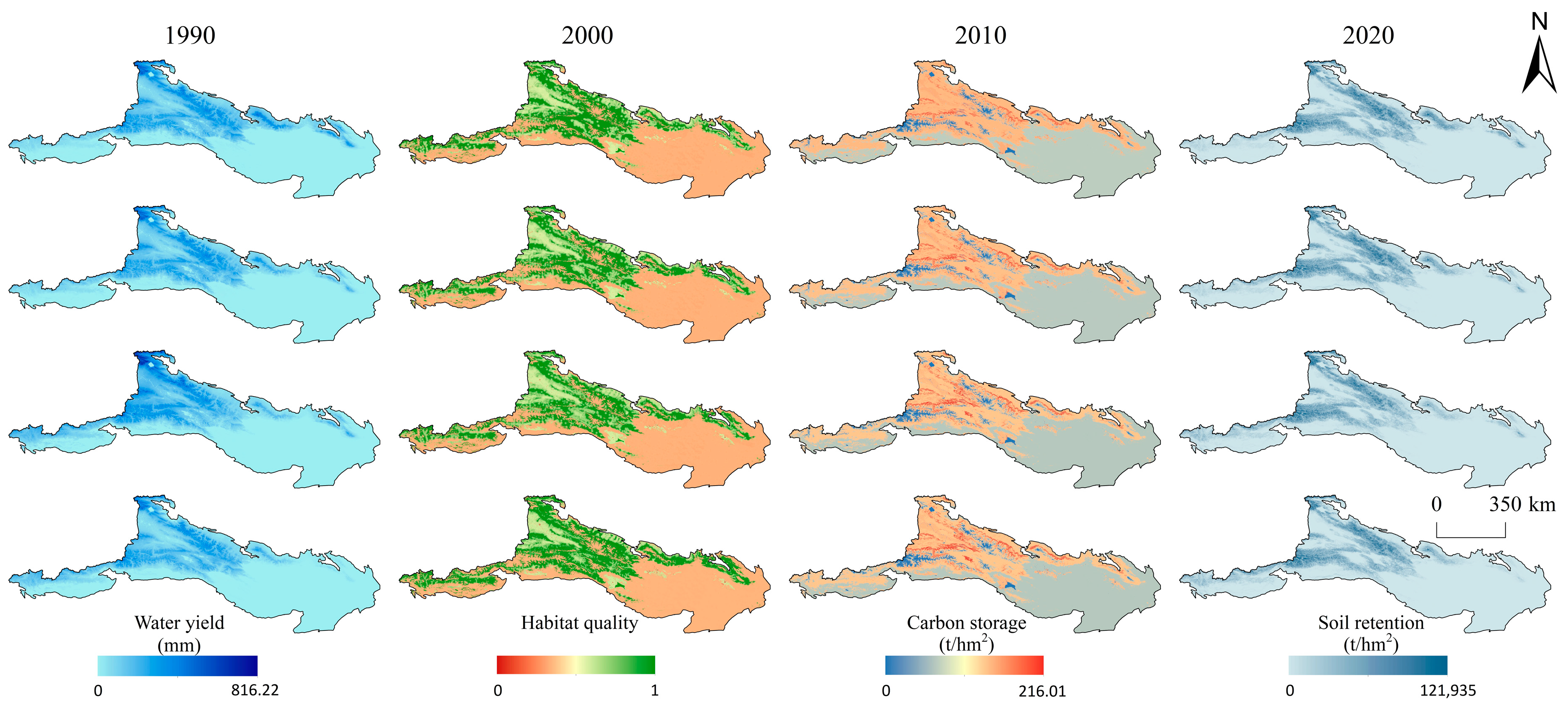
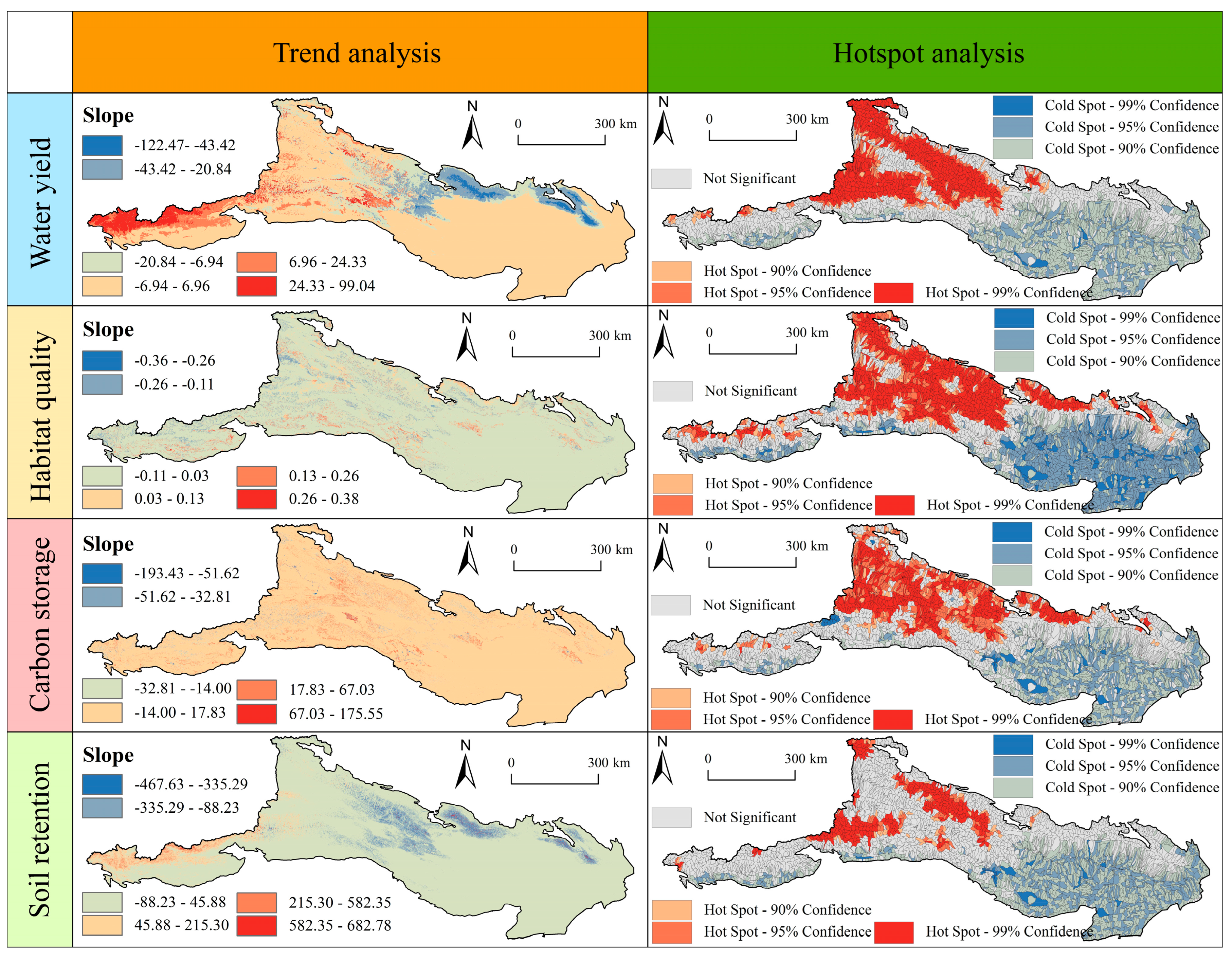
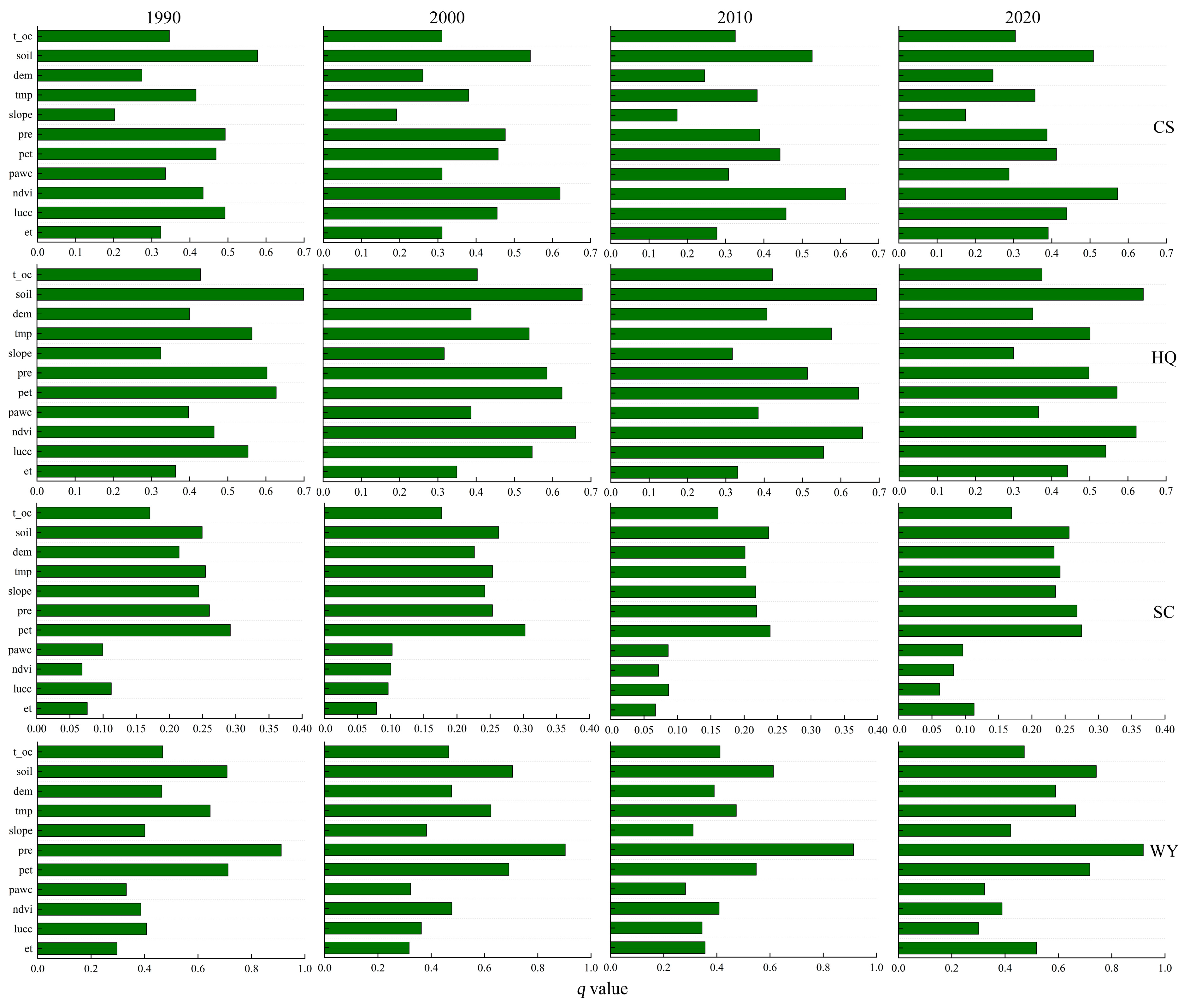
4.1. Characteristics and Driving Factors of ES Changes

The spatial distribution of the ESs in the Tianshan region from 1990 to 2020 is shown in Figure 2. The spatial patterns for the WY, HQ, CS, and SC were similar, with the highest values predominantly found in grassland zones, forest zones, river valleys, and intermountain basins. All of these areas had good vegetation cover. The lowest values were concentrated in desert zones and snow/ice zones. Figure 3 shows that from 1990 to 2020, the WY and SC values increased near the Harketawu Mountains, with SC increasing more rapidly. However, near the Bogda Mountains and Blikun Mountains, the WY and SC decreased, with SC decreasing more rapidly, while the HQ and CS remained relatively stable. In the hot spot analysis, the WY, HQ, CS, and SC exhibited similar spatial distributions, with hot spots primarily located in the BoroHoro Ula Mountains and Yilianhabierga Mountains, and cold spots mainly located in the Turpan Basin.
Figure 4 indicates that the precipitation was the primary explanatory factor for the WY (q = 0.91, the same for the average value below). The amount of precipitation received directly determines the water volume in the surface and groundwater reserves, thereby affecting the WY. Therefore, the changes in the WY were closely related to the changes in the precipitation and areas with high precipitation corresponded to areas with a high WY. Soil type, potential evapotranspiration (PET), and the normalized difference vegetation index (NDVI) were the primary explanatory factors for the HQ (q = 0.68, q = 0.62, and q = 0.60, respectively). The soil type determines the growth environment of plant roots, thereby affecting plant growth and distribution. Different soil types have different water retention capacities, air permeabilities, and nutrient contents, which directly affect plant growth and habitat quality. The PET is the sum of plant transpiration and soil evaporation, reflecting the plant’s water demand and water utilization in the environment. A high PET may indicate a greater water demand by plants, while a low PET may indicate sufficient water supply in the environment [56]. Therefore, there is a close relationship between the PET and habitat quality. The NDVI is an indicator used for assessing vegetation cover. High NDVI values typically indicate dense vegetation, while low NDVI values indicate sparse vegetation. Vegetation cover is directly related to habitat quality [57], because abundant vegetation can improve soil quality, protect water sources, and maintain the ecological balance. Changes in the HQ were closely related to the changes in these factors. The primary drivers of CS were the soil type and NDVI (q = 0.53 and q = 0.56), which both affect the HQ and CS capacity by influencing vegetation growth, soil nutrient cycling, and water retention. The main factor influencing SC was the PET (q = 0.28) and changes in the SC were closely related to changes in the PET.

4.2. Correlation Analysis

4.2.1. The Relationship between ESs

The interaction between the four ES functions of WY, HQ, CS, and SC, were investigated using the R4.0 software and Pearson correlation analysis (Figure 5). From 1990 to 2020, the WY, HQ, CS, and SC, all displayed a synergistic relationship. Significant positive correlations were observed between the water yield and CS, HQ, and SC, with correlation coefficients of 0.54, 0.65, and 0.52, respectively. Similarly, soil conservation showed significant positive correlations with CS and HQ, with correlation coefficients of 0.23 and 0.29, respectively. Habitat quality was significantly positively correlated with CS, with a correlation coefficient of 0.8. The correlations between WY, HQ, CS, and SC, in the Tianshan Mountains, in 2000, 2010, 2015, and 2020, were consistent with the trends in 1990.

4.2.2. Spatial Pattern of the Trade-Offs and Synergies between the ESs

The spatial heterogeneity of the trade-offs and synergies among the ES pairs was revealed by the GWR results (Figure 6). The spatial pattern was relatively consistent in regard to the correlation analysis results, indicating that the spatial synergy ratios for CS–HQ, WY–HQ, and WY–SC were much higher than the spatial trade-off ratios. They generally exhibited synergy effects throughout the entire Tianshan region, suggesting that these ES pairs were dominated by spatial synergy, which manifested as strong correlations in Figure 5. In contrast, the spatial trade-off proportions in terms of CS–SC, CS–WY, and HQ–SC, were approximately equal to the spatial synergy proportions. The trade-off regions in terms of CS–SC were mainly concentrated in the eastern and western parts of the Turpan Basin, while those of CS–WY were mainly concentrated in the Halketagh Mountains, the Ili-Habirga Mountains, and the central Turpan Basin. The trade-off regions in terms of HQ–SC were mainly concentrated near the Bogda Mountains. These results indicate that these ES pairs exhibited certain spatial trade-off characteristics, which manifested as weaker correlations in Figure 5.

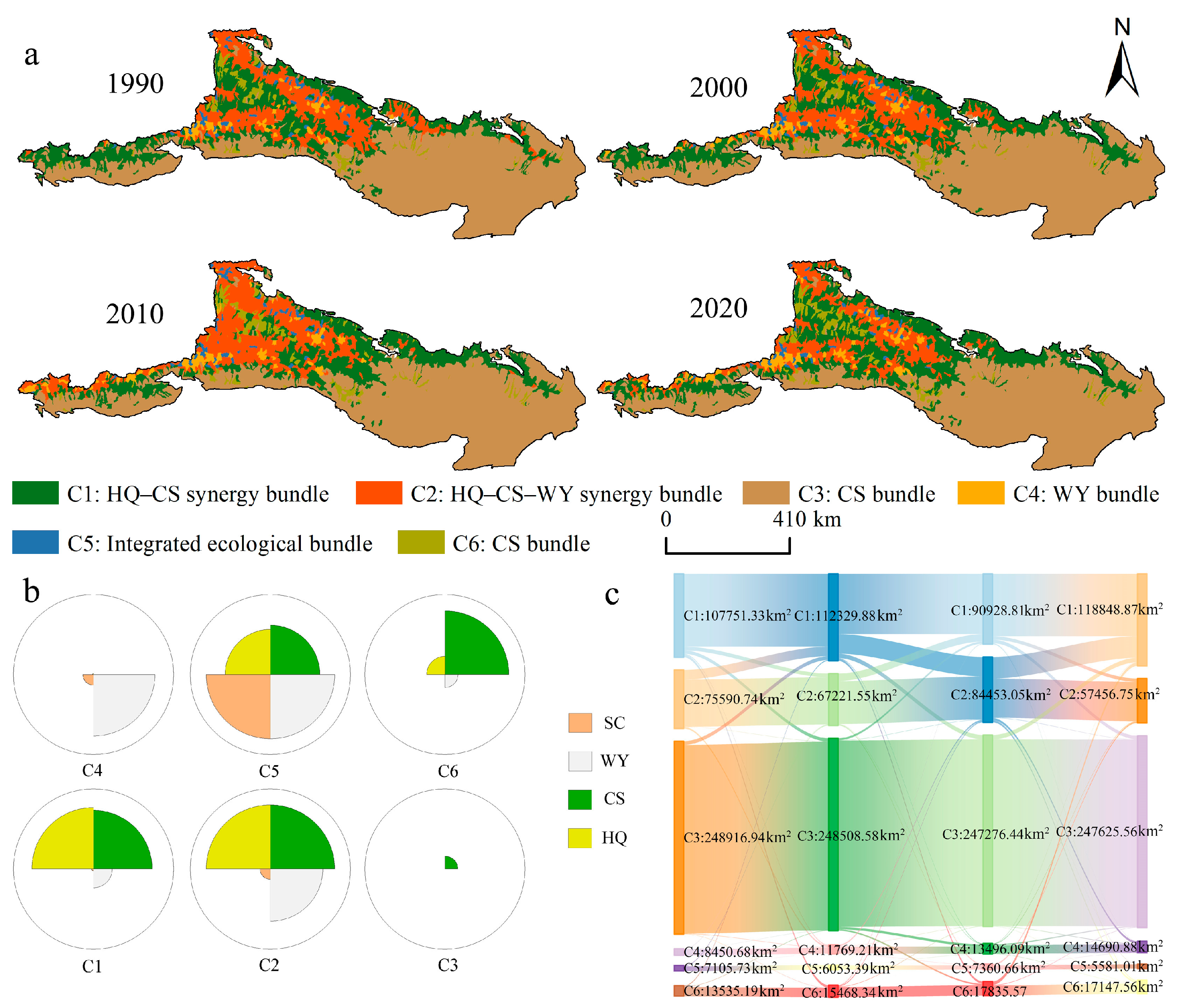
4.3. Distribution and Characteristics of ES Bundles

The SOM process identified six ES bundles (Figure 7): the HQ–CS synergy bundle (C1), the HQ–CS–WY synergy bundle (C2), the CS bundle (C3), the WY bundle (C4), the integrated ecological bundle (C5), and the CS bundle (C6). It was found that C1 was mainly distributed in the low altitude Ili Basin and the plains surrounding five mountain ranges; C2 was predominantly found in the high-altitude Bolokenu, Harketawu, and Yilianhabierga Mountains, while C3 was primarily located in desert regions (such as the Turpan Basin); C4 and C5 were scattered in the central and northwestern parts of the Tianshan Mountains; and C6 was mainly distributed in the Ili Basin. According to Figure 7c, from 1990 to 2000, the C1, C4, and C6 areas displayed an expanding trend, while C2 and C5 displayed a decreasing trend, and C3 remained relatively unchanged. The most prominent transition during this period occurred from C2 to C1. From 2000 to 2010, the C2, C4, C5, and C6 areas displayed an expanding trend, while C1 displayed a decreasing trend, and C3 remained relatively unchanged. The most prominent transition during this period occurred from C1 to C2 and C3. From 2010 to 2020, the change trends in terms of the six ES bundles were the same as those from 1990 to 2000, with C1, C4, and C6 displaying an expanding trend, C2 and C5 displaying a decreasing trend, and C3 remaining relatively unchanged. The most prominent transition during this period occurred from C2 to C1. Overall, from 1990 to 2000, the C1, C4, and C6 areas increased by 11097.54, 6240.2, and 3612.37 km2, respectively, while the C2 and C5 areas decreased by 18,133.99 and 1524.72 km2, respectively, and the C3 area remained relatively unchanged.

5. Discussion

5.1. The Characteristics of ES Interactions

Effective environmental management fundamentally relies on understanding the complex interactions among ESs [58]. The spatial coexistence of various ESs creates unique ES bundles, which are vital for regional functional zoning, managing land multifunctionality, and improving regional ESs [59,60,61]. Ecosystem services also exhibit spatial thermal erosion, a characteristic often linked to heterogeneity in the spatial distribution of socio-ecological factors [62]. Therefore, determining the relationships among ESs is a prerequisite for sustainable management. The spatial distribution investigation of ESs in the Tianshan Mountains showed similar patterns for the WY, SC, CS, and HQ, with high ES values mainly found in grassland belts, forest belts, river valleys, and intermountain basins. Furthermore, the high altitudes and rugged terrain in these regions elevate moist airflows, leading to abundant precipitation, while the high altitudes also reduce evaporation and transpiration. Additionally, precipitation and snowmelt from the mountains supply water for vegetation and organisms in the surrounding areas. The high water supply capacity and conservation potential of these regions were influenced by their topographic and climatic features. Consequently, the dominant synergies at the watershed scale were CS–HQ, WY–HQ, and WY–SC, which manifested as different combinations of ES bundles among these ESs. The synergistic effects among these ESs are aligned with previous research findings [19,27,58]. The quality of the ESs in the Turpan Basin and its surrounding areas was relatively poor, primarily due to the combined effects of the extreme arid climatic conditions, soil degradation, human activities, insufficient vegetation cover, and the region’s unique geological and soil conditions. These factors interacted, collectively forming a fragile foundation for the region’s ES capacity in areas where cold spots in terms of ES pairs were also primarily concentrated. Therefore, for ecological restoration and sustainable development in the Turpan Basin, comprehensive measures should be taken to improve water resource management, restore vegetation cover, and control inappropriate human activities, thereby enhancing the region’s ES capacity.

5.2. Implications for Ecosystem Management

Understanding the influence of each driving factor on ESs is crucial for explaining changes in ESs and developing appropriate response strategies. Given the nonlinear and complex effects of natural factors on ESs, traditional linear regression is inadequate for quantifying the impact of one ES on another [63]. Consequently, we employed the GD method to assess the influence of driving factors on the ESs. The GD results indicated that precipitation had the most significant impact on the WY values, aligning with the findings by Huang et al. [64], who identified precipitation as a key driving factor for several ESs.
Due to the rugged terrain, low temperatures, steep slopes, and remote locations, mountainous regions are vulnerable to climate change, especially in arid and semi-arid areas, where climate change has become a major threat to the existing land uses and vegetation cover [65]. High temperatures increase evaporation, restricting plant growth in arid regions [66]. The Tianshan Mountains have a dry climate, with evaporation exceeding precipitation, and the resulting drought inhibits vegetation growth, and is one of the negative effects of climate warming. Increased precipitation improves hydrological conditions, regulates the water cycle, and enhances the WY [67]. Changes in water and heat conditions affect vegetation types and growth, influencing soil retention capacity, and abnormal fluctuations in precipitation present a risk of soil erosion [37,38]. It is necessary to develop mitigation and adaptation strategies to improve the water supply capacity of environmental and social resources, address climate change, and achieve sustainable development. Previous studies [68] have shown that human disturbance has a minor impact on environmental protection because most studies have been conducted in key ecological functional zones in Xinjiang, where economic activities are restricted. Economic growth promotes ecological governance, and the establishment of nature reserves protects ecosystems and biodiversity. However, the impact of grazing on the environment should be taken seriously. Large areas of grassland are used as pastures, and while moderate grazing promotes plant growth, overgrazing leads to the degradation of grassland shrubs, making mountain ecological restoration difficult. It is necessary to improve grazing patterns, maintain appropriate grazing capacity, and minimize the impact on mountain grassland ESs.

5.3. Limitations of This Study and Future Prospects

This study had some limitations that should be recognized. In terms of the ES assessment, there was a lack of validation, and no uncertainty analysis of the simulation results produced by the InVEST model was carried out. The simulation accuracy of the InVEST model is primarily constrained by data availability, spatial data accuracy, and modeling techniques [69]. Additionally, in this study, the model parameters were calibrated mainly based on relevant studies from the same or adjacent regions [31,70,71]. However, due to differences in the data sources and regional variations, there are certain biases in the estimation results. Therefore, future research needs to adopt mechanistic models based on biophysical processes and high-quality data, while considering the localization of model parameters and model validation to ensure the accuracy of the simulation results [72]. Compared to studies involving long-term continuous spatiotemporal dynamics, this research only analyzes changes in the Tianshan region over four specific years. The time scale is non-continuous, focusing on a few static time periods, which may lead to misinterpretations of the interrelationships among the ecosystem services [73]. Future research should consider examining the interrelationships among ecosystem services over long-term, continuous time periods to reduce the uncertainty in the results. In terms of the research scale, this study considered the collaborative supply capacity of ESs on the small watershed scale, which is where ecohydrological processes occur. Considering that ESs and their trade-offs/synergies are scale dependent [74], future research should explore the threshold effects of the interactions between ESs on multiple scales, including remote sensing pixels and administrative units [75].
Additionally, it is important to recognize the significance of desert and snow/ice zones, which were categorized as “low value areas”. These regions play crucial roles in biodiversity and ecosystem functions, such as in regard to albedo effects on climate and water resources [76]. Their importance should not be neglected. Future research should explore their contributions to overall ecosystem services [77].
Climate change is likely to affect the intensity, seasonality, and variability of precipitation. It will also influence the type of precipitation (snow or rain) and the speed of snowmelt [78]. These changes will impact water availability, erosion, and landslide risks. Although current projections do not allow for firm conclusions concerning specific localities under various scenarios, it is essential to consider these factors in future research and management strategies [79].
Finally, the LUCC categorization used in this study, even when supplemented with NDVI data, does not provide detailed information on land and forest management, forest types, or forest health [80]. These factors have implications for carbon storage and vulnerability to fires, pests, and other disturbances. Future research should incorporate more detailed land and forest management data to improve the accuracy and relevance of ecosystem service assessments [81].

6. Conclusions

This study used various methods, such as GWR, the GD method, and SOMs, to explore the interactions and driving factors in terms of ESs in the Tianshan region. The main conclusions were as follows. (1) The four ESs of WY, HQ, CS, and SC, had similar spatial distribution patterns, with high-value areas mainly concentrated in the grassland and forest zones of the mountains, as well as river valleys and intermountain basins, while low-value areas were concentrated in desert and snow/ice zones. (2) From 1990 to 2020, the WY and SC increased near the Harketawu Mountains and decreased near the Bogda Mountains and Blikun Mountains, while the HQ and CS remained largely unchanged. The hot spots in terms of the WY, HQ, CS, and SC were mainly concentrated in the BoroHoro Ula Mountains and Yilianhabierga Mountains, while the cold spots were mainly concentrated in the Turpan Basin. (3) Precipitation was the primary explanatory factor for the WY; the soil type, PET, and NDVI were the primary explanatory factors for the HQ; the soil type and NDVI were the primary explanatory factors for CS; and the PET was the primary explanatory factor for SC. (4) Overall, there was a synergistic relationship between the WY, HQ, CS, and SC, with the strongest synergistic relationships between CS–HQ, WY–HQ, and WY–SC, with average correlation coefficients of 0.81, 0.60, and 0.52, respectively. The spatial trade-offs and synergies in terms of ES pairs exhibited spatial heterogeneity, with some ES pairs having trade-off areas, such as CS–WY trade-offs, that were mainly concentrated in the Harketawu Mountains, Yilianhabierga Mountains, and central Turpan Basin. The HQ–SC trade-off areas were mainly concentrated near the Bogda Mountains. (5) The SOM analysis identified six ES bundles. From 1990 to 2000, the C1, C4, and C6 areas expanded, while the C2 and C5 areas decreased, and the C3 area remained unchanged. From 2000 to 2010, the C2, C4, C5, and C6 areas expanded, while the C1 area decreased, and the C3 area remained unchanged. From 2010 to 2020, the trends in terms of the six ES bundles were the same as those from 1990 to 2000. Overall, from 1990 to 2000, the C1, C4, and C6 areas increased, while the C2 and C5 areas decreased, and the C3 area remained largely unchanged, indicating that the ES management priorities varied across different regions.

Author Contributions

Conceptualization, W.C. and R.W.; methodology, W.C. and R.W.; software, X.L. and T.L.; validation, W.C. and R.W.; formal analysis, Z.H.; investigation, X.L.; resources, W.C. and R.W.; data curation, W.C., R.W. and Y.Z. (Yukun Zhang); writing, W.C. and R.W.; writing—review and editing, W.C., R.W. and X.L.; visualization, W.C. and R.W.; supervision, W.C., R.W. and Y.Z. (Yu Zheng); project administration, X.L.; funding acquisition, X.L. All authors have read and agreed to the published version of the manuscript.

Funding

This research was funded by the Field Observation and Monitoring Data Collection and Analysis Services for Typical Areas in the Headwaters of the Tarim River—Pilot Research on the Construction of Xinjiang Natural Resources Monitoring and Early Warning System Project; the Technology Innovation Center for Ecological Monitoring and Restoration of Desert-Oasis, MNR (2023KFKTA001); the research on the suitability evaluation and application of natural resources in Xinjiang based on surface matrix (LTSJ-ZFCG-2024-021); China Geological Survey Project (DD20230112, DD20230514).

Data Availability Statement

The data presented in this study are available on request from the corresponding author.

Conflicts of Interest

The authors declare that there are no conflicts of interest.

References

  1. Daily, G.C. Nature’s Services: Societal Dependence on Natural Ecosystems (1997); The Future of Nature; Yale University Press: New Haven, CT, USA, 2013; pp. 454–464. [Google Scholar]
  2. Costanza, R.; d’Arge, R.; De Groot, R.; Farber, S.; Grasso, M.; Hannon, B.; Limburg, K.; Naeem, S.; O’neill, R.V.; Paruelo, J.; et al. The value of the world’s ecosystem services and natural capital. Nature 1997, 387, 253–260. [Google Scholar] [CrossRef]
  3. Rozas-Vásquez, D.; Fürst, C.; Geneletti, D.; Almendra, O. Integration of ecosystem services in strategic environmental assessment across spatial planning scales. Land Use Policy 2018, 71, 303–310. [Google Scholar] [CrossRef]
  4. Dittrich, A.; Seppelt, R.; Václavík, T.; Cord, A.F. Integrating ecosystem service bundles and socio-environmental conditions—A national scale analysis from Germany. Ecosyst. Serv. 2017, 28, 273–282. [Google Scholar] [CrossRef]
  5. Gao, J.B.; Zuo, L.Y. Revealing ecosystem services relationships and their driving factors for five basins of Beijing. J. Geogr. Sci. 2021, 31, 111–129. [Google Scholar] [CrossRef]
  6. Redhead, J.W.; May, L.; Oliver, T.H.; Hamel, P.; Sharp, R.; Bullock, J.M. National scale evaluation of the InVEST nutrient retention model in the United Kingdom. Sci. Total Environ. 2018, 610, 666–677. [Google Scholar] [CrossRef]
  7. Yao, T.; Weiping, Z.; Hui, Z.; Yu, S. A review on principle and application of the InVEST model. Ecol. Sci. 2015, 34, 204–208. [Google Scholar]
  8. Young, C.J.; Don, L.S. Assessment of economic value of ecosystem service by using InVEST model in South Korea. Int. J. Environ. Sci. Dev. 2017, 8, 815–818. [Google Scholar] [CrossRef]
  9. Leh, M.D.; Matlock, M.D.; Cummings, E.C.; Nalley, L.L. Quantifying and mapping multiple ecosystem services change in West Africa. Agric. Ecosyst. Environ. 2013, 165, 6–18. [Google Scholar] [CrossRef]
  10. Li, Y.G.; Liu, W.; Feng, Q.; Zhu, M.; Yang, L.S.; Zhang, J.T. Quantitative Assessment for the Spatiotemporal Changes of Ecosystem Services, Tradeoff-Synergy Relationships and Drivers in the Semi-Arid Regions of China. Remote Sens. 2022, 14, 239. [Google Scholar] [CrossRef]
  11. Huang, M.Y.; Wang, Q.L.; Yin, Q.; Li, W.H.; Zhang, G.Z.; Ke, Q.J.; Guo, Q. Analysis of Ecosystem Service Contribution and Identification of Trade-Off/Synergy Relationship for Ecosystem Regulation in the Dabie Mountains of Western Anhui Province, China. Land 2023, 12, 1046. [Google Scholar] [CrossRef]
  12. Saidi, N.; Spray, C. Ecosystem services bundles: Challenges and opportunities for implementation and further research. Environ. Res. Lett. 2018, 13, 113001. [Google Scholar] [CrossRef]
  13. Xu, F.; Chen, S.G.; Wang, X.Y.; Wang, X.R. Spatio-Temporal Changes and Trade-Offs/Synergies among Ecosystem Services in Beijing from 2000 to 2020. Forests 2023, 14, 2314. [Google Scholar] [CrossRef]
  14. Niu, T.; Yu, J.X.; Yue, D.P.; Yang, L.Z.; Mao, X.Q.; Hu, Y.H.; Long, Q.Q. The Temporal and Spatial Evolution of Ecosystem Service Synergy/Trade-Offs Based on Ecological Units. Forests 2021, 12, 992. [Google Scholar] [CrossRef]
  15. Raudsepp-Hearne, C.; Peterson, G.D.; Bennett, E.M. Ecosystem service bundles for analyzing tradeoffs in diverse landscapes. Proc. Natl. Acad. Sci. USA 2010, 107, 5242–5247. [Google Scholar] [CrossRef]
  16. Fu, B.J.; Zhang, L.W.; Xu, Z.H.; Zhao, Y.; Wei, Y.P.; Skinner, D. Ecosystem services in changing land use. J. Soils Sediments 2015, 15, 833–843. [Google Scholar] [CrossRef]
  17. Cord, A.F.; Bartkowski, B.; Beckmann, M.; Dittrich, A.; Hermans-Neumann, K.; Kaim, A.; Lienhoop, N.; Locher-Krause, K.; Priess, J.; Schröter-Schlaack, C.; et al. Towards systematic analyses of ecosystem service trade-offs and synergies: Main concepts, methods and the road ahead. Ecosyst. Serv. 2017, 28, 264–272. [Google Scholar] [CrossRef]
  18. Turner, K.G.; Odgaard, M.V.; Bocher, P.K.; Dalgaard, T.; Svenning, J.C. Bundling ecosystem services in Denmark: Trade-offs and synergies in a cultural landscape. Landsc. Urban Plan. 2014, 125, 89–104. [Google Scholar] [CrossRef]
  19. Yang, G.F.; Ge, Y.; Xue, H.; Yang, W.; Shi, Y.; Peng, C.H.; Du, Y.Y.; Fan, X.; Ren, Y.; Chang, J. Using ecosystem service bundles to detect trade-offs and synergies across urban-rural complexes. Landsc. Urban Plan. 2015, 136, 110–121. [Google Scholar] [CrossRef]
  20. Yao, J.; He, X.Y.; Chen, W.; Ye, Y.; Guo, R.C.; Yu, L.Z. A local-scale spatial analysis of ecosystem services and ecosystem service bundles in the upper Hun River catchment, China. Ecosyst. Serv. 2016, 22, 104–110. [Google Scholar] [CrossRef]
  21. Lyu, R.F.; Clarke, K.C.; Zhang, J.M.; Feng, J.L.; Jia, X.H.; Li, J.J. Spatial correlations among ecosystem services and their socio-ecological driving factors: A case study in the city belt along the Yellow River in Ningxia, China. Appl. Geogr. 2019, 108, 64–73. [Google Scholar] [CrossRef]
  22. Dou, H.S.; Li, X.B.; Li, S.K.; Dang, D.L.; Li, X.; Lyu, X.; Li, M.Y.; Liu, S.Y. Mapping ecosystem services bundles for analyzing spatial trade-offs in inner Mongolia, China. J. Clean. Prod. 2020, 256, 120444. [Google Scholar] [CrossRef]
  23. Gou, M.M.; Li, L.; Ouyang, S.; Wang, N.; La, L.M.; Liu, C.F.; Xiao, W.F. Identifying and analyzing ecosystem service bundles and their socioecological drivers in the Three Gorges Reservoir Area. J. Clean. Prod. 2021, 307, 127208. [Google Scholar] [CrossRef]
  24. Feng, Z.; Jin, X.R.; Chen, T.Q.; Wu, J.S. Understanding trade-offs and synergies of ecosystem services to support the decision-making in the Beijing?Tianjin?Hebei region. Land Use Policy 2021, 106, 105446. [Google Scholar] [CrossRef]
  25. Karimi, J.D.; Corstanje, R.; Harris, J.A. Understanding the importance of landscape configuration on ecosystem service bundles at a high resolution in urban landscapes in the UK. Landsc. Ecol. 2021, 36, 2007–2024. [Google Scholar] [CrossRef]
  26. Zuo, L.Y.; Gao, J.B. Investigating the compounding effects of environmental factors on ecosystem services relationships for Ecological Conservation Red Line areas. Land Degrad. Dev. 2021, 32, 4609–4623. [Google Scholar] [CrossRef]
  27. Zheng, D.F.; Wang, Y.H.; Hao, S.; Xu, W.J.; Lv, L.T.; Yu, S. Spatial -temporal variation and tradeoffs/synergies analysis on multiple ecosystem services: A case study in the Three -River Headwaters region of China. Ecol. Indic. 2020, 116, 106494. [Google Scholar] [CrossRef]
  28. Quintas-Soriano, C.; García-Llorente, M.; Norström, A.; Meacham, M.; Peterson, G.; Castro, A.J. Integrating supply and demand in ecosystem service bundles characterization across Mediterranean transformed landscapes. Landsc. Ecol. 2019, 34, 1619–1633. [Google Scholar] [CrossRef]
  29. Hong, Y.Y.; Ding, Q.; Zhou, T.; Kong, L.Q.; Wang, M.Y.; Zhang, J.Y.; Yang, W. Ecosystem service bundle index construction, spatiotemporal dynamic display, and driving force analysis. Ecosyst. Health Sustain. 2020, 6, 1843972. [Google Scholar] [CrossRef]
  30. Youcun, L.; Keqin, J.; Kui, Z.; Yan, L.; Tianding, H.; Yu, Z. The response of precipitation to global climate change in the Tianshan Mountains, China. J. Glaciol. Geocryol. 2017, 39, 748–759. [Google Scholar]
  31. Yayan, L.; Xiaoliang, X.; Jicai, L.; Xiaohua, F.; Luyuan, L. Research on the spatio-temporal variation of carbon storage in the Xinjiang Tianshan Mountains based on the InVEST model. Arid Zone Res. 2022, 39, 1896–1906. [Google Scholar]
  32. Xia, C.H.; Hu, Z.C.; Xi, C.; Ming, C.W. The new methodology of geomorphologic zonalization in Xinjiang based on geographical grid. Geogr. Res. 2008, 27, 481–492+725–726. [Google Scholar]
  33. Chen, Y.; Li, W.; Deng, H.; Fang, G.; Li, Z. Changes in Central Asia’s Water Tower: Past, Present and Future. Sci. Rep. 2016, 6, 35458. [Google Scholar] [CrossRef] [PubMed]
  34. Groombridge, B.; Jenkins, M. Global Biodiversity: Earth’s Living Resources in the 21st Century; World Conservation Press: Cambridge, UK, 2000. [Google Scholar]
  35. Yang, J.; Huang, X. 30 m annual land cover and its dynamics in China from 1990 to 2019. Earth Syst. Sci. Data Discuss. 2021, 2021, 1–29. [Google Scholar]
  36. Li, M.Y.; Liang, D.; Xia, J.; Song, J.X.; Cheng, D.D.; Wu, J.T.; Cao, Y.L.; Sun, H.T.; Li, Q. Evaluation of water conservation function of Danjiang River Basin in Qinling Mountains, China based on InVEST model. J. Environ. Manag. 2021, 286, 112212. [Google Scholar] [CrossRef]
  37. Guo, F.; Liu, X.; Mamat, Z.; Zhang, W.; Xing, L.; Wang, R.; Luo, X.; Wang, C.; Zhao, H. Analysis of spatiotemporal variations and influencing factors of soil erosion in the Jiangnan Hills red soil zone, China. Heliyon 2023, 9, e19998. [Google Scholar] [CrossRef]
  38. Yuan, J.L.; Liu, X.H.; Li, H.Y.; Wang, R.; Luo, X.P.; Xing, L.Y.; Wang, C.; Zhao, H.H. Assessment of Spatial-Temporal Variations of Soil Erosion in Hulunbuir Plateau from 2000 to 2050. Land 2023, 12, 1214. [Google Scholar] [CrossRef]
  39. Sharp, R.; Tallis, H.; Ricketts, T.; Guerry, A.D.; Wood, S.A.; Chaplin-Kramer, R.; Nelson, E.; Ennaanay, D.; Wolny, S.; Olwero, N. InVEST+ VERSION+ User’s Guide. Nat. Cap. Proj. 2016. [Google Scholar]
  40. Peng, J.; Yang, Y.; Liu, Y.X.; Hu, Y.N.; Du, Y.Y.; Meersmans, J.; Qiu, S.J. Linking ecosystem services and circuit theory to identify ecological security patterns. Sci. Total Environ. 2018, 644, 781–790. [Google Scholar] [CrossRef]
  41. Budyko, M.I. Climate and Life; Academic Press: Cambridge, MA, USA, 1974. [Google Scholar]
  42. Xu, J.Y.; Chen, J.X.; Liu, Y.X.; Fan, F.F. Identification of the geographical factors influencing the relationships between ecosystem services in the Belt and Road region from 2010 to 2030. J. Clean. Prod. 2020, 275, 124153. [Google Scholar] [CrossRef]
  43. Yin, L.C.; Wang, X.F.; Feng, X.M.; Fu, B.J.; Chen, Y.Z. A Comparison of SSEBop-Model-Based Evapotranspiration with Eight Evapotranspiration Products in the Yellow River Basin, China. Remote Sens. 2020, 12, 2528. [Google Scholar] [CrossRef]
  44. Zhang, H.; Deng, W.; Zhang, S.Y.; Peng, L.; Liu, Y. Impacts of urbanization on ecosystem services in the Chengdu-Chongqing Urban Agglomeration: Changes and trade-offs. Ecol. Indic. 2022, 139, 108920. [Google Scholar] [CrossRef]
  45. Zhai, T.L.; Zhang, D.; Zhao, C.C. How to optimize ecological compensation to alleviate environmental injustice in different cities in the Yellow River Basin? A case of integrating ecosystem service supply, demand and flow. Sustain. Cities Soc. 2021, 75, 103341. [Google Scholar] [CrossRef]
  46. Getis, A.; Ord, J.K. The analysis of spatial association by use of distance statistics. Geogr. Anal. 1992, 24, 189–206. [Google Scholar] [CrossRef]
  47. Wang, J.F.; Li, X.H.; Christakos, G.; Liao, Y.L.; Zhang, T.; Gu, X.; Zheng, X.Y. Geographical detectors-based health risk assessment and its application in the neural tube defects study of the Heshun Region, China. Int. J. Geogr. Inf. Sci. 2010, 24, 107–127. [Google Scholar] [CrossRef]
  48. Erfu, D.; Yahui, W. Spatial heterogeneity and driving mechanisms of water yield service in the Hengduan Mountain region. Acta Geogr. Sin. 2020, 75, 607–619. [Google Scholar]
  49. Wang, J.-F.; Hu, Y. Environmental health risk detection with GeogDetector. Environ. Model. Softw. 2012, 33, 114–115. [Google Scholar] [CrossRef]
  50. Chen, S.L.; Liu, X.T.; Yang, L.; Zhu, Z.H. Variations in Ecosystem Service Value and Its Driving Factors in the Nanjing Metropolitan Area of China. Forests 2023, 14, 113. [Google Scholar] [CrossRef]
  51. Fotheringham, A.S.; Charlton, M.; Brunsdon, C. Measuring Spatial Variations in Relationships with Geographically Weighted Regression. In Recent Developments in Spatial Analysis: Spatial Statistics, Behavioural Modelling, and Computational Intelligence; Fischer, M.M., Getis, A., Eds.; Springer: Berlin/Heidelberg, Germany, 1997; pp. 60–82. [Google Scholar]
  52. Bennett, E.M.; Peterson, G.D.; Gordon, L.J. Understanding relationships among multiple ecosystem services. Ecol. Lett. 2009, 12, 1394–1404. [Google Scholar] [CrossRef]
  53. Gollini, I.; Lu, B.; Charlton, M.; Brunsdon, C.; Harris, P. GWmodel: An R package for exploring spatial heterogeneity using geographically weighted models. arXiv 2013, arXiv:1306.0413. [Google Scholar]
  54. Chen, L.H.; Ma, Y. A Framework for Assessing Trade-Offs and Synergies in Green Space System Services Based on Ecosystem Services Bundles. Forests 2023, 14, 1614. [Google Scholar] [CrossRef]
  55. Wehrens, R.; Buydens, L.M. Self-and super-organizing maps in R: The Kohonen package. J. Stat. Softw. 2007, 21, 1–19. [Google Scholar] [CrossRef]
  56. Yan, L.; Kairui, Z. Effects of NDVI/Land-Use on Evapotranspiration in the Loess Plateau. Yellow River 2021, 43, 68–73. [Google Scholar]
  57. Jiangzhu, L.; Qing, L.; Ting, Z. Spatial scale enhancement and spatio-temporal variation of evapotranspiration based on the relationship between K_c and NDVI. South–North Water Transf. Water Sci. Technol. 2023, 21, 417–426. [Google Scholar]
  58. Xia, H.; Yuan, S.F.; Prishchepov, A.V. Spatial-temporal heterogeneity of ecosystem service interactions and their social-ecological drivers: Implications for spatial planning and management. Resour. Conserv. Recycl. 2023, 189, 106767. [Google Scholar] [CrossRef]
  59. Rodríguez-Loinaz, G.; Alday, J.G.; Onaindia, M. Multiple ecosystem services landscape index: A tool for multifunctional landscapes conservation. J. Environ. Manag. 2015, 147, 152–163. [Google Scholar] [CrossRef]
  60. He, L.J.; Xie, Z.Y.; Wu, H.Q.; Liu, Z.; Zheng, B.F.; Wan, W. Exploring the interrelations and driving factors among typical ecosystem services in the Yangtze river economic Belt, China. J. Environ. Manag. 2024, 351, 119794. [Google Scholar] [CrossRef]
  61. Shen, J.S.; Li, S.C.; Liang, Z.; Liu, L.B.; Li, D.L.; Wu, S.Y. Exploring the heterogeneity and nonlinearity of trade-offs and synergies among ecosystem services bundles in the Beijing-Tianjin-Hebei urban agglomeration. Ecosyst. Serv. 2020, 43, 101103. [Google Scholar] [CrossRef]
  62. Xu, J.; Wang, S.; Xiao, Y.; Xie, G.D.; Wang, Y.Y.; Zhang, C.S.; Li, P.; Lei, G.C. Mapping the spatiotemporal heterogeneity of ecosystem service relationships and bundles in Ningxia, China. J. Clean. Prod. 2021, 294, 126216. [Google Scholar] [CrossRef]
  63. Li, S.K.; Li, X.B.; Dou, H.S.; Dang, D.L.; Gong, J.R. Integrating constraint effects among ecosystem services and drivers on seasonal scales into management practices. Ecol. Indic. 2021, 125, 107425. [Google Scholar] [CrossRef]
  64. Huang, F.X.; Zuo, L.Y.; Gao, J.B.; Jiang, Y.; Du, F.J.; Zhang, Y.B. Exploring the driving factors of trade-offs and synergies among ecological functional zones based on ecosystem service bundles. Ecol. Indic. 2023, 146, 109827. [Google Scholar] [CrossRef]
  65. Xu, S.N.; Liu, Y.F.; Wang, X.; Zhang, G.X. Scale effect on spatial patterns of ecosystem services and associations among them in semi-arid area: A case study in Ningxia Hui Autonomous Region, China. Sci. Total Environ. 2017, 598, 297–306. [Google Scholar] [CrossRef]
  66. Lu, Y.Y.; Xu, X.L.; Zhao, J.H.; Han, F. Spatiotemporal Evolution of Mountainous Ecosystem Services in an Arid Region and Its Influencing Factors: A Case Study of the Tianshan Mountains in Xinjiang. Land 2022, 11, 2164. [Google Scholar] [CrossRef]
  67. Ning, T.T.; Feng, Q.; Li, Z.; Li, Z.X.; Xi, H.Y.; Yang, L.S.; Chang, X.G. Precipitation changes and its interaction with terrestrial water storage determine water yield variability in the world’s water towers. Sci. Total Environ. 2023, 880, 163285. [Google Scholar] [CrossRef] [PubMed]
  68. Li, F.Z.; Yin, X.X.; Shao, M. Natural and anthropogenic factors on China’s ecosystem services: Comparison and spillover effect perspective. J. Environ. Manag. 2022, 324, 116064. [Google Scholar] [CrossRef]
  69. Agudelo, C.A.R.; Bustos, S.L.H.; Moreno, C.A.P. Modeling interactions among multiple ecosystem services. A critical review. Ecol. Model. 2020, 429, 109103. [Google Scholar] [CrossRef]
  70. Xu, W.; Yang, L.; Chen, X.; Gao, Y.; Wang, L. Carbon storage, spatial distribution and the influence factors in Tianshan forests. Chin. J. Plant Ecol. 2016, 40, 364–373. [Google Scholar]
  71. Han, C.; Zheng, J.; Wang, Z.; Yu, W. Spatiotemporal variation and multiscenario simulation of carbon storage in terrestrial ecosystems in the Turpan-Hami Basin based on PLUS-InVEST model. Arid Land Geogr. 2024, 47, 260–269. [Google Scholar]
  72. Li, R.; Li, H.; Wu, F.; Zhao, M.; Wang, S.; Sun, X. Study on the spatial differentiation pattern and driving force of ecosystem services in Qinghai Lake Basin. Ecol. Environ. Sci. 2024, 33, 301–309. [Google Scholar]
  73. Liu, R.; Niu, X.; Wang, B.; Song, Q. InVEST model-based spatiotemporal analysis of water supply services in the Zhangcheng District. Forests 2021, 12, 1082. [Google Scholar] [CrossRef]
  74. Qiu, J.X.; Carpenter, S.R.; Booth, E.G.; Motew, M.; Zipper, S.C.; Kucharik, C.J.; Loheide, S.P.; Turner, A.G. Understanding relationships among ecosystem services across spatial scales and over time. Environ. Res. Lett. 2018, 13, 054020. [Google Scholar] [CrossRef]
  75. Zheng, H.; Wang, L.J.; Wu, T. Coordinating ecosystem service trade-offs to achieve win-win outcomes: A review of the approaches. J. Environ. Sci. 2019, 82, 103–112. [Google Scholar] [CrossRef]
  76. Liu, Y.; Kong, L.; Jiang, C.; Zhang, X.; Ouyang, Z. Accounting of value of ecosystem services in the desert: An example of the Kubuqi Desert ecosystem. Front. Earth Sci. 2024, 11, 1247367. [Google Scholar] [CrossRef]
  77. Ba, Z.; Du, H.; Hasi, E.; Lu, X. Changes in land use and ecosystem service value in desert areas of China after reform and opening up. Front. Earth Sci. 2023, 11, 1251605. [Google Scholar] [CrossRef]
  78. Thackeray, C.W.; Derksen, C.; Fletcher, C.G.; Hall, A. Snow and climate: Feedbacks, drivers, and indices of change. Curr. Clim. Chang. Rep. 2019, 5, 322–333. [Google Scholar] [CrossRef]
  79. Kaufmann, R.K.; Pretis, F. An empirical estimate for the snow albedo feedback effect. Clim. Chang. 2023, 176, 107. [Google Scholar] [CrossRef]
  80. Zhao, S.; Tu, K.; Ye, S.; Tang, H.; Hu, Y.; Xie, C. Land use and land cover classification meets deep learning: A review. Sensors 2023, 23, 8966. [Google Scholar] [CrossRef]
  81. Jia, B.; Guo, W.; He, J.; Sun, M.; Chai, L.; Liu, J.; Wang, X. Topography, diversity, and forest structure attributes drive aboveground carbon storage in different forest types in Northeast China. Forests 2022, 13, 455. [Google Scholar] [CrossRef]
Figure 1. Study area. Note: the map is based on a standard map from the standard map service website GS (2019) 1823 of the Ministry of Natural Resources. The boundary of the base map has not been modified.
Forests 15 01678 g001
Figure 2. Spatiotemporal changes to the ecosystem services in the Tianshan Mountains from 2000 to 2020.
Forests 15 01678 g002
Figure 3. Characteristics of ecosystem services.
Forests 15 01678 g003
Figure 4. The explanatory power of ecosystem service drivers.
Forests 15 01678 g004
Figure 5. Correlations between ecosystem service pairs (* p < 0.05; ** p < 0.01; *** p < 0.001).
Forests 15 01678 g005
Figure 6. Spatial synergies and trade-offs between the ES pairs.
Forests 15 01678 g006
Figure 7. (a) The temporal and spatial patterns of ES bundles. (b) The relative composition and size of ESs in the ES bundles. (c) The mutual conversion area of different ES bundles from 1990 to 2020 (left column to right column).
Forests 15 01678 g007
Table 1. Data sources and description.
DataDescriptionData Sources
Land-use type data in 1990, 2000, 2010, and 2020The spatial resolution is 30 m.https://zenodo.org
(accessed on 23 October 2023)
Temperature (°C)Monthly average temperature data with a 1 km resolution.National Tibetan Plateau Scientific Data Center https://data.tpdc.ac.cn/home (accessed on 8 May 2023)
Precipitation (mm)Monthly average precipitation data with a 1 km resolution.
Evapotranspiration (mm)Annual evapotranspiration data with a 1 km resolution.
Potential evapotranspiration (mm)Annual potential evapotranspiration data with a 1 km resolution.
Normalized difference vegetation index (NDVI)The spatial resolution is 1 km.
Soil dataUsed to calculate the plant available water capacity (PAWC) and soil erodibility factor.
Soil typeThe spatial resolution is 1 km.
Rainfall erosivity factorReflects the rainfall intensity and time in the study area.Obtained by calculating the rainfall data
Carbon density (t/hm2)Used to calculate the CS.Based on relevant literature
Digital elevation model (DEM) (m)Used to calculate the slope direction and slope, terrain fluctuation, with a spatial resolution of 30 m.Geospatial Data Cloud
https://www.gscloud.cn
(accessed on 19 May 2023)
Gross domestic product (GDP)The GDP value of the county-level unit with a 1 km resolution.Data Center for Resources and Environmental Sciences, Chinese Academy of Sciences https://www.resdc.cn
(accessed on 18 May 2023)
Population gridded dataset (POP)The population value of the county-level unit with a 1 km resolution.
Road dataUsed to calculate the distance to the road.OpenStreetMap Data extract https://www.openstreetmap.org
(accessed on 24 April 2023)
River network dataUsed to calculate the distance to the river channel.
The location of the governmentUsed to calculate the distance to the government.National Geographic Information Resources Catalog Service System
https://www.webmap.cn
(accessed on 11 April 2023)
Disclaimer/Publisher’s Note: The statements, opinions and data contained in all publications are solely those of the individual author(s) and contributor(s) and not of MDPI and/or the editor(s). MDPI and/or the editor(s) disclaim responsibility for any injury to people or property resulting from any ideas, methods, instructions or products referred to in the content.

