Abstract
Climate warming is impacting vegetation productivity and plant leaf phenology, but the precise climate drivers and windows of key leaf phenological phases, such as emergence and fall, are still not well understood. Recent intensive computational approaches based on pinpointing the optimal climate window of leaf phenophases by maximizing the signal could help to advance in this question. In this study, we assess the climate variables, the climate windows, and the type of relationship (linear or nonlinear) that drive leaf emergence and fall in 21 deciduous and 13 evergreen woody plant species inhabiting two sites in Mediterranean Spain. We used precipitation, solar radiation, and different temperature measures, including forcing and chilling, as climate variables. We found that forcing variables were the best predictors of leaf phenology, but other temperature variables, as well as precipitation and radiation, were also important. However, chilling was not a good predictor. Most selected models showed nonlinear relationships. The best thresholds for calculating forcing were different from those commonly used. In addition, the best climate window for leaf phenology was species-specific and contingent on climatic and phenological conditions. This optimum climate window often covered longer periods than those usually considered in phenology studies. Our approach could be used to assess and better forecast future plant phenological responses to climate warming.
1. Introduction
The study of plant phenology, i.e., the recording of recurring events or phenophases, has gained increasing attention over the past decades as a tool to monitor the impacts of climate warming on terrestrial ecosystems [1,2,3]. For instance, several studies have documented an earlier leaf onset in response to climate warming, either using direct observations [4] or indirect remote-sensing data [5]. Direct relationships were found between the timing of budburst and secondary growth cessation in spring and the timing of the previous senescence onset [6]. Leaf flushing and senescence have also been found to be related to the onset and cessation of xylem growth and carbon sink limitations [7,8]. In the case of forests, the relationships between phenology and environmental variables have been shown to be complex and involve the interactions between the photoperiod and temperature, as triggers of budburst in some tree species [9,10,11].
Understanding the key climate drivers of leaf emergence and fall in woody plant species is critical to assess the impacts of phenological changes on ecosystem productivity and to model the feedbacks between the biosphere and the climate system [12,13]. However, determining which climatic variables determine the timing of key phenological phases in woody plants, such as leaf emergence or leaf fall, is challenging because of the complexity of the physiological processes involved. In order for leaf flushing to occur, dormancy must first be overcome, which is divided into three phases: dormancy induction; endo-dormancy, controlled by plant-endogenous factors and characterized by the inability to grow, even under favorable environmental conditions; and eco-dormancy, a period during which emergence occurs if environmental conditions are suitable [14]. Each of these periods is affected by different factors. Although dormancy induction is generally associated with the photoperiod and decreasing temperatures, a minimum period of low temperatures (chilling) is required for overcoming endo-dormancy, and an increase in temperature (forcing) is required for overcoming the eco-dormancy phase [14]. However, the different phases of dormancy are interdependent so that a greater exposure to chilling may result in less forcing required for leaf emergence, and, conversely, greater forcing may compensate for less exposure to chilling [15,16]. Likewise, chilling and forcing requirements may be fulfilled simultaneously, indicating that there is no temporal separation between these two phenophases [17]. Furthermore, these patterns of climate–dormancy relationships may vary widely among species and climate types [2,18]. The complexity of these relationships has led to sometimes contradictory results. For example, an advance or a delay in the leaf emergence because of climate change has been predicted, depending on the weight given to forcing or chilling, respectively [2,19]. There are also different ways to measure these variables, which can lead to different results [2]. Compared to leaf’s spring phenology, the analysis of the variables behind leaf senescence or fall is even more difficult because the processes underlying it are still poorly understood [20]. Therefore, additional efforts are needed to better understand the variables that drive leaf phenology in trees and shrubs.
Nowadays, large amounts of data can be analyzed because of the rapid development of computational power. This increased data-processing capacity allows us to study phenology–climate relationships, using intensive data analysis methods. Among the more recently developed methods, one that stands out is the one that focuses on finding the temporal window with daily resolution, during which the relationship between a phenological variable and the climate is the maximum. This type of analysis reduces the noise and maximizes the climate signal, which can allow us to better understand the variables that drive phenology. Among the programs developed for such analyses is the R [21] package climwin [22,23], which allows the comparison of thousands of alternative models, with the goal of finding the climate window, usually with daily temporal resolution, that maximizes the relationships (both linear and nonlinear) between phenological events (e.g., the date of the leaf emergence) and climatic variables (including chilling and forcing effects).
Leaf phenology studies generally use absolute (fixed) climate windows [17,24]. However, because phenology responds to climate cues and other environmental signals and not to a particular calendar date, a relative approach, i.e., finding the relative climate window that maximizes the phenology–climate relationship, is an analysis that can help to pinpoint the climate windows of key leaf phenological events. Whereas the absolute approach seeks to identify the start and end dates of the climate window, the relative approach seeks to identify the time separating the start or end of the climate window from the phenological event under consideration.
In this work, we analyzed the relationships of two leaf phenological phases (emergence and fall) with the climate, using both relative and absolute approaches (finding the most suitable climate window of each phenological event), in 34 woody species inhabiting two Mediterranean sites. The species studied are of both agricultural and forestry interests and include 21 deciduous and 13 evergreen tree, vine, and shrub species. We conducted an intensive analysis, testing different climatic variables (the mean, maximum, and minimum temperatures; radiation; precipitation; and accumulation of forcing and chilling by employing different thresholds), relationships (linear or nonlinear), and climate windows, to find the best-fitted models of leaf phenology. Our specific objectives are (I) to detect the main climate variables that drive leaf phenology; (II) to pinpoint the climate windows in which the relationship between the climate and phenology is maximized; (III) to discern if the type of relationship between the climate and leaf phenology is linear or nonlinear, which will have clear implications for the impacts of climate warming on the vegetation’s aboveground productivity; and (IV) to compare the results obtained from the relative and absolute climate window approaches.
2. Materials and Methods
2.1. Leaf Phenology Data
Long-term phenological series from Roquetas (40°49′ N, 00°31′ E; 50 m a.s.l.) and Cardedeu (41°34′ N, 2°21′ E; 193 m a.s.l.), both located in northeastern Spain, were used. In Roquetas, the data were collected by the “Observatorio del Ebro”, a research institute, founded in 1904, that has been collecting phenological information since 1908, although it was not until 1943 that the acquisition of phenological information was systematized by the Spanish Meteorological Agency (AEMET) and has been obtained continuously since that year to the present [25]. From this database (for the period 1950–2001), previously re-analyzed by Gordo and Sanz [25] and Camarero et al. [26], we have used two phenophases: leaf emergence (the appearance of the first leaves in at least 50% of the individuals of the same species) and leaf fall (branches that have lost half of their leaves in at least 50% of the individuals of the same species; for evergreen plants, this leaf loss refers to the oldest leaf cohort, i.e., the set of leaves belonging to the previous year for species with leaf lifespans of less than 24 months, or to the oldest year for leaves with longer lifespans). Given the number of species measured, the different longevities of the species, and the length of the period in which phenology measurements were made, sampling conditions vary between species and years (e.g., the age and number of individuals are not constant between species), but in general, phenology was measured for at least 3–5 individuals, taking the dominant phenological state among all the individuals as the phenology value. Wherever possible, the same individuals were sampled across years, although the reduced longevity of some species means that dying individuals had to be substituted. We have used the leaf emergence data of 26 plant species (13 cultivated and 13 native) and the leaf fall data of 20 plant species (10 cultivated and 10 native; Table S1). The climate is Mediterranean, with a strong influence of the sea (the coast is located 15 km from the study site). The average total annual precipitation was 544 mm, and the average annual temperature was 17.4 °C (climate diagrams in Figure S1).
In Cardedeu, the long-term phenological data were recorded by one person (Pere Comas) from 1952 to 2000. They were obtained from AEMET and were previously analyzed by Peñuelas et al. [27] in a study focused on analyzing the effects, on animal and plant phenologies, of the rise in temperature that has occurred here in recent decades. Here, the data were collected from 1953 to 2000. From this database, we have used only the leaf emergence data of 7 plant species, 2 cultivated and 5 native. The climate is Mediterranean, with the coast located 8 km from the study site. The average total annual precipitation was 658 mm, and the average annual temperature was 14.8 °C (see climate diagrams in Figure S1). Therefore, Cardedeu is cooler and wetter than Roquetas.
2.2. Climate Data
For the Roquetas site, we used the daily precipitation (Prec) and daily average, maximum, and minimum temperature (Temp, Tmax, and Tmin, respectively) data taken from “Observatorio del Ebro” (data available at http://www.obsebre.es, accessed on 21 February 2022). For the Cardedeu site, because of the lack of long and complete series of local meteorological data from weather stations located in the study area, we used daily climate series (Prec, Temp, Tmax, and Tmin data) from the 0.1°-gridded Spain02-v5 dataset [28,29]. This dataset faithfully reproduces climatological features, including weather extremes, thanks to the dense network of weather stations used and covers from 1950 to the present. More than 3000 precipitation stations and over 250 temperature stations located across Spain were used to build the Spain02-v5 dataset. Because of the lack of daily radiation (Rad) data at the two study sites, this variable was obtained from the 0.1°-gridded E-OBS v23.1e dataset [30].
2.3. Statistical Analyses
For each phenological variable (leaf emergence and fall) of a given plant species, different types of relationships (linear, quadratic, cubic, or logarithmic) were tested with the different climatic variables, using the climwin R package [22,23] (R version 4.2.1). Temp, Tmax, Tmin, and Rad were used as climatic variables. Chilling and forcing accumulation variables were also tested. Chilling variables were calculated as the sum of days (of the climate window considered) when the temperature (calculated separately for Temp, Tmax, and Tmin) was lower than 0, 5, 10, or 15 °C [17]. For the calculation of the chilling variables, in addition to the upper threshold given, a lower threshold of 0 °C is usually set so that only those days with a temperature within the range defined by the two thresholds were summed [10,31]. However, this was not necessary for our study sites, where freezing temperatures are rare. As forcing variables, the degree-days were calculated for temperatures (also separately for Temp, Tmax, and Tmin) higher than 5, 10, 15, or 20 °C (base temperature), i.e., the difference between the base temperature and the daily value of the temperature variable considered was summed for all the days of the period considered (the climate window) [17]. A total of 12 chilling and 12 forcing variables were used, one for each temperature threshold (0, 5, 10, or 15 °C and 5, 10, 15, or 20 °C, for chilling and forcing, respectively) and type of temperature (Temp, Tmax, or Tmin) considered.
We calculated, for each species, phenological variable, climate variable, and type of relationship, the time period in which the phenology–climate relationship is maximal (the best climate window). To select the best climate window between a phenological species series (leaf emergence and fall) and a given climate variable (Temp, Tmax, Tmin, Rad, chilling, and forcing) separately for each type of relationship (linear, quadratic, cubic, or logarithmic), all the possible models were first fitted. In each model, a different climate window with a daily temporal resolution was tested (Figure S2).
Then, for each species and phenological variable, the model (with a given climate variable, climate window, and type of relationship) that minimizes ΔAICc was chosen [32]. ΔAICc is the difference between the corrected Akaike information criterion (AICc) of the selected model and the AICc of the baseline model. For the phenological series of each species, we fitted both simple models, including a single climate variable in each model (in this case, the baseline model was the null model that contained only the intercept), and multiple models, including two climate variables in each model. To create the multiple models, we first introduced the climate variable and the climate window with the lowest ΔAICc (i.e., we started from the best simple model, which was, in this case, the baseline model) and then added, one by one, the rest of the possible variables in order to fit all the possible two-variable models, and for each variable, we tested all the possible climate windows, using the different types of relationships. Three-variable models were also tested but ultimately discarded because little additional variability was explained by the third variable in all the species. We used the mean (for the minimum and maximum temperatures) and the total or sum (for precipitation, chilling, and forcing) of each time window considered as the aggregate statistic. For example, if we fit models that relate phenology (the response variable) to precipitation (Prec as a predictor), Prec = (Prec1, Prec2, …, Precn) will be a vector of n values, where each Preci represents the total precipitation during the considered climate window in year i, and i is an index such that i ∈ {1, 2, …, n}. We established a minimum period of 15 days between windows opening and closing. We set a minimum period of 15 days between opening and closing windows. This minimum period allows a reduction in the computational time and avoids obtaining excessively small windows that have no biological significance but that, by chance, obtain a low ∆AICc value. Calculations were performed using absolute climate windows and repeated using relative climate windows for comparison. Relative climate windows measure the time, in the number of days before each biological record, when the relationship is maximal (for example, between 1 and 20 days before budbreak), while absolute climate windows measure the time with fixed calendar dates (e.g., from March 3 to 20). The fact that the timing of the leaf emergence and leaf fall of a given species varies from year to year, means that if we use relative windows, the dates covering the climate windows will also vary from year to year, whereas if we use absolute windows, the dates will remain constant each year.
The large numbers of models that are fitted to test all the possible climate windows increase the possibility of obtaining models with low ∆AICc values by chance. To solve this problem, randomization tests were performed on all the models obtained using 1000 repetitions. The randomization test determines the expected distribution of ΔAICc values in a dataset where no response to the climate exists and provides a probability value (p AICc) that determines the likelihood that the ΔAICc value of the selected model has occurred by chance [23]. Only those variables for which p AICc < 0.1 are shown in the Results Section. As randomization tests require a high degree of computational power, we used the “Magerit” high-performance computer at Universidad Politécnica de Madrid (www.cesvima.upm.es, Madrid, Spain, last access on 25 September 2024) to carry out these analyses.
3. Results
The models fitted to analyze phenology–climate relationships gave markedly different results, depending on whether relative or absolute climate windows were used. Using relative climate windows, the goodness of fit of the models was much higher, with an average explained variability (R2) of 0.81 (see values with interannual variation in Table 1), compared to 0.44 for average R2 values in the cases of simple models using absolute climate windows (see R2SM values in Table 2, Table 3 and Table 4). Furthermore, the most important variable in using relative climate windows was radiation, for all the species (Table 1), while the most important climatic variable was species-specific, using absolute climate windows, with temperature variables generally being more relevant (Table 2, Table 3 and Table 4).

Table 1.
Relative climate windows (RWO and RWC), coefficients (coef.), and explained variability (R2) of linear models relating radiation to the leaf emergence at the Roquetas site. Results are based on relative climate windows and are compared using actual climate data (with inter-daily and interannual variabilities) and daily means for the whole study period (with inter-daily but not interannual variability). Relative open (RWO) and closed (RWC) windows show the best relative climate window, measured in the number of days before the leaf emergence for the opening (RWO) and closing (RWC) windows considered. Leaf habit (LH): D, deciduous; E, evergreen.
Table 2.
The best multiple models (with two predictors) relating the leaf emergence in Roquetas to climate variables. For each predictor, the type of relationship (function) and whether any transformation of the predictor has been performed (upper and lower) are shown. Upper indicates that the predictor has been transformed to degree-days (forcing). In these cases, the threshold at which the degree-days are counted is shown. Lower indicates that the predictor measures the number of days where the temperature is below the indicated threshold (chilling). The variability values explained by the simple model (R2SM, only with the first predictor) and by the full model (R2) are also shown. Temp, Tmax, Tmin, Prec, and Rad refer to the mean, maximum, and minimum temperatures; precipitation; and solar radiation, respectively. See the model coefficients in Table S2 and the climate windows considered in Figure 1.
Table 3.
The best multiple models (with two predictors) relating the leaf fall in Roquetas to climate variables. For each predictor, the type of relationship (function) and whether any transformation of the predictor has been performed (upper and lower) are shown. Upper indicates that the predictor has been transformed to degree-days (forcing). In these cases, the threshold at which the degree-days are counted is shown. Lower indicates that the predictor measures the number of days where the temperature is below the indicated threshold (chilling). The variability values explained by the simple model (R2SM, only with the first predictor) and by the full model (R2) are also shown. Temp, Tmax, Tmin, Prec, and Rad refer to the mean, maximum, and minimum temperatures; precipitation; and solar radiation, respectively. See the model coefficients in Table S2 and the climate windows considered in Figure 2.
Table 4.
The best multiple models (with two predictors) relating the leaf emergence in Cardedeu to climate variables. For each predictor, the type of relationship (function) and whether any transformation of the predictor has been performed (upper and lower) are shown. Upper indicates that the predictor has been transformed to degree-days (forcing). In these cases, the threshold at which the degree-days are counted is shown. Lower indicates that the predictor measures the number of days where the temperature is below the indicated threshold (chilling). The variability values explained by the simple model (R2SM, only with the first predictor) and by the full model (R2) are also shown. Temp, Tmax, Tmin, Prec, and Rad refer to the mean, maximum, and minimum temperatures; precipitation; and solar radiation, respectively. See the model coefficients in Table S2 and the climate windows considered in Figure 3.
The climatic variables, which have a strong seasonal component, with a more or less constant intra-annual (inter-daily) pattern from one year to another, especially for variables such as temperature or radiation, lead to the value of the climatic variable being strongly conditioned by the period considered (Figure S3). For example, if we consider a generic model that relates the leaf emergence to radiation, using the relative approach; where E = (E1, E2, …, En) will be a vector of n values, where each Ei represents the day of the year (DOY) of the leaf emergence in year i, and i is an index such that i ∈ {1, 2, …, n}; where the best climate window is at a given distance (dist. in Figure S3, corresponding to the values of the RWC in Table 1) with respect to E, which is constant over the years (only in the relative approach); where Rad = (Rad1, Rad2, …, Radn) will be a vector of n values, where each Radi represents the mean radiation during the considered climate window (CWi) in year i; the model is then relating the emergence values E1, E2, …, En to the radiation values Rad1, Rad2, …, Radn corresponding to the climate windows CW1, CW2, …, CWn. Therefore, as observed in the conceptual model shown in Figure S3, when we follow the relative approach, a delay in phenology (E2 > E1) leads to a lower mean value for the climate window considered (Rad2 < Rad1) and vice versa, resulting in a strong non-causal phenology–climate relationship. The non-causality of these results is evidenced by repeating the analyses, using a relative approach and eliminating the interannual variability of the climate (but leaving the intra-annual variability of the climate and the interannual variability of the phenology; see results without interannual variability in Table 1). Effectively, these analyses without interannual climate variability and, thus, without any causal relationship, give an even better goodness of fit (note that all the models without interannual climate variability explain 100% of the variability in the response variable, i.e., R2 = 1). Such non-causal relationships are not possible when using absolute windows, where the start and end dates of the climate window remain constant each year. For this reason, only the results obtained using absolute climate windows are shown in the remaining analyses.
The final models fitted with two climatic predictors (or one, when the second variable did not show a significant reduction in AICc) generally explained most of the variability in leaf emergence dates, with mean R2 values of 0.57 in Roquetas (Table 2) and 0.81 in Cardedeu (Table 4). The leaf-fall models showed the lowest mean R2 value (0.53; Table 3). The mean autocorrelations of the leaf emergence time (the correlation between the date of the emergence in one year and the date of the emergence in the previous year) were 0.28 (R2 = 0.11) and 0.31 (R2 = 0.16) in Roquetas and Cardedeu, respectively, while that of the leaf fall in Roquetas was 0.16 (R2 = 0.07). In addition, the average correlation between the date of the leaf emergence and the date of the subsequent leaf fall was 0.19 (R2 = 0.08).
The most important climatic variables for both leaf emergence and fall were species-specific, although, in general, the temperature variables, measured as degree-days (the sum of degrees above a certain threshold, which also turned out to be species-specific, i.e., forcing variables), were the most important drivers and explained the most variability. On the other hand, chilling variables, i.e., those measuring the number of days with temperatures below a certain threshold, generally showed the opposite relationship to that expected, as a higher number of days with temperatures below the threshold was associated with a delay in the leaf emergence (e.g., in Ceratonia siliqua and Erica ciliaris, among others; see variables in Table 2, Table 3 and Table 4 and the directions of their influences in Figures S4–S9).
Most of the climate–phenology relationships were nonlinear (Table 2, Table 3 and Table 4), generally due to the fact that the response of the phenology was more pronounced when the climate took extreme values, while the sensitivity of the phenology was lower when the climate took intermediate values (see, e.g., Cedrus sp., Citrus × limon, and Genista scorpius, among others, in Figure S4). In other cases, however, the nonlinear relationship was due to the fact that the leaf emergence (fall) was advanced (delayed) when the climate values were around an optimum range, outside of which the leaf emergence (fall) was delayed (advanced). This was the case for Acacia sp., Hedera sp., or Malus domestica for the leaf emergence (Figure S5) and for Ficus carica, Malus domestica, or Prunus armeniaca for the leaf fall (Figure S6).
The period during which climate influences leaf phenology is shown in Figure 1, Figure 2 and Figure 3. This period was species-specific for leaf emergence, although, in general, in the case of thermal windows, it included the period before the leaf emergence and extended up to the beginning of the year (Figure 1 and Figure 3). In the cases of the precipitation and solar radiation, or when temperature was included in the second predictor, the climate windows were more variable and could include the end of the previous growing season as well as the winter and autumn before the leaf emergence.
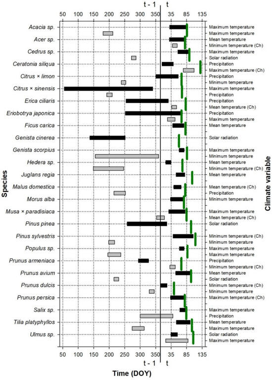
Figure 1.
Periods showing the strongest relationship (the best absolute climate window) between the leaf emergence date and climate variables for the species studied at the Roquetas site. The green vertical lines indicate the average emergence date for each plant species (see the exact values for the day of the year, DOY, on the abscissa axis, in Table S3); t and t − 1 indicate whether the considered period belongs to the growth year or to the previous year, respectively. The color indicates the importance of the variable for the leaf emergence: periods with black color were the first variables introduced to the model, which produced the greatest reduction in the AICc value with respect to the null model; periods with gray color were the second variables introduced to the model, which produced the greatest reduction in the AICc value with respect to the model with a climatic variable. If the climate has been transformed to a chilling variable (the number of days in which the temperature is below the considered threshold during the climate window), it is indicated with (Ch). DOY is the Julian calendar day of the year.
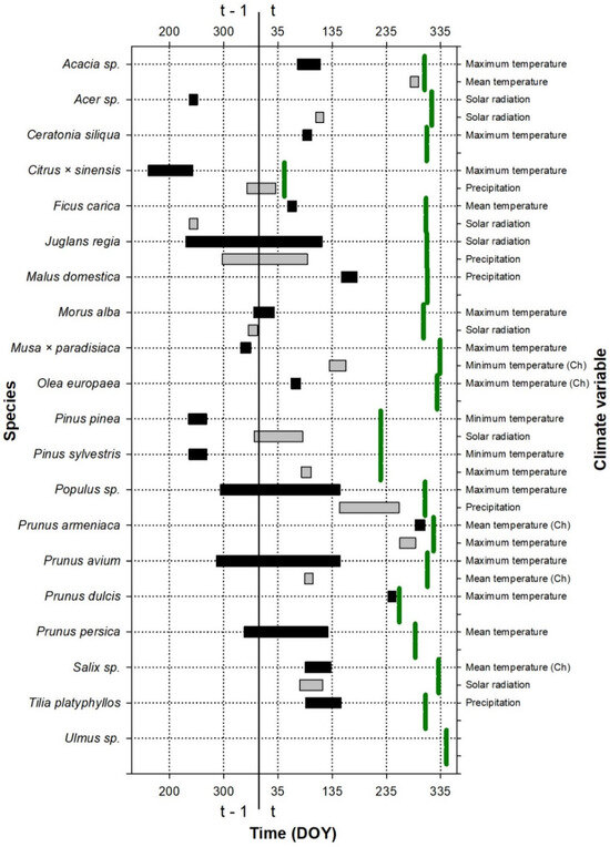
Figure 2.
Periods showing the strongest relationship (the best absolute climate window) between the leaf fall date and climate variables for the species studied at the Roquetas site. The green vertical lines indicate the average leaf fall date for each species (see the exact values for the day of the year, DOY, on the abscissa axis, in Table S3); t and t − 1 indicate whether the considered period belongs to the growth year or to the previous year, respectively. The color indicates the importance of the variable for leaf fall: periods with black color were the first variables introduced to the model, which produced the greatest reduction in the AICc value with respect to the null model; periods with gray color were the second variables introduced to the model, which produced the greatest reduction in the AICc value with respect to the model with a climatic variable. If the climate has been transformed to a chilling variable (the number of days in which the temperature is below the considered threshold during the climate window), it is indicated with (Ch). DOY is the Julian calendar day of the year.
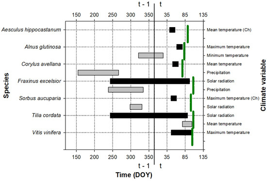
Figure 3.
Periods showing the strongest relationship (the best absolute climate window) between the leaf emergence date and climate variables for the species studied at the Cardedeu site. The green vertical lines indicate the average emergence date for each species (see the exact values for the day of the year, DOY, on the abscissa axis, in Table S3); t and t − 1 indicate whether the considered period belongs to the growth year or to the previous year, respectively. The color indicates the importance of the variable for the leaf emergence: periods with black color were the first variables introduced to the model, which produced the greatest reduction in the AICc value with respect to the null model; periods with gray color were the second variables introduced to the model, which produced the greatest reduction in the AICc value with respect to the model with a climatic variable. If the climate has been transformed to a chilling variable (the number of days in which the temperature is below the considered threshold during the climate window), it is indicated with (Ch). DOY is the Julian calendar day of the year.
The climate window during which the climate influenced the leaf fall did not include the pre-fall period, except in some species (e.g., Acacia sp. or Prunus armeniaca; Figure 2), but it was, in general, related to the period before the leaf emergence and the early growing season.
4. Discussion
4.1. Absolute or Relative Climate Windows
When an event is determined by the climate prior to it, the use of climate windows relative to the time of the event could be the most appropriate approach. For example, relative climate windows have been used in animal biology [33]. However, our results show that this is not an appropriate approach when working with variables that show a strong seasonal pattern.
The results obtained using relative climate windows (with interannual variation) suggest that the mean solar radiation occurring between 118 and 231 days (mean values for all the species in the RWC and RWO, respectively) prior to the leaf emergence, i.e., the previous autumn, determines the date of the leaf emergence. This result could have biological significance, as these are the dates when buds are developing, which could determine the leaf phenology of the following year. However, as shown in Table 1 (see results without interannual variability within this table), there is a strong non-causal relationship between the intra-annual trends of radiation and phenology. In addition, if there was a real causal relationship, we should have found it using absolute climate windows, especially considering that these windows no longer cover the climate just before the event (which would justify the use of relative windows) but the climate that occurred more than 100 days before. Therefore, the relative approach leads to non-causal relationships that invalidate it as an appropriate method for studying phenology–climate relationships.
4.2. Not Only Forcing Is Important
Temperature has been widely recognized as the major climate driver of the spring leaf-out in non-tropical zones [2,34,35]. The temperature variables considered as drivers of leaf emergence are those that measure forcing and chilling [17,36]. In line with this, our results show that temperature, measured as degree-days (forcing), was the most important variable determining the timing of the leaf emergence. However, contrary to expectations, chilling was not generally found to be a variable related to phenology in the fitted models, and when a relationship was found, the direction of the relationship was the opposite of that expected, i.e., the more days of low temperature, the greater the delay in phenology. This result may be related to the observational nature of the data. In an experimental study with temperature control, it is possible to separate forcing and chilling requirements, but in an observational study, this separation is much more complex. In this sense, an autumn or winter with relatively low temperatures will often be followed by a cooler spring because of temperature autocorrelation or persistent atmospheric circulation patterns, which can lead to a shorter time to reach chilling requirements but a longer time to reach forcing requirements. On the other hand, plants adjust the timing of the leaf emergence to maximize the growing season but minimize the likelihood of late frost damage [37,38]. However, temperatures in the study areas are very mild, with average winter temperatures close to 10 °C (Figure S1). This may mean that the chilling requirements of the different species in the study area are minimal or non-existent because of the low probability of frost damage. Previous studies on Mediterranean climates and species also show no relationship between chilling and the leaf emergence date [39]. In any case, a weak relationship between chilling and the leaf emergence does not mean that there is no causal relationship between this climatic variable and other phenological factors, such as the leaf emergence rate [39].
The existing literature on the climatic variables driving leaf fall points to temperature as the main driver, indicating that higher temperatures lead to a delay in the leaf fall [40,41]. However, our results suggest a more complex relationship, where generally high temperatures at the beginning of the growing season lead not only to an earlier leaf emergence but also to an earlier leaf fall (this would be the case for Acacia sp., Ceratonia siliqua, or Prunus avium, among others). Keenan and Richarson [42] point out the complexity of the generally misunderstood factors influencing the leaf fall and indicate that, in line with our results, the timing of the leaf fall is conditioned by the timing of the leaf emergence and, we add, is, therefore, determined by the same climatic factors that drive leaf emergence. This could be because of different mechanisms, such as leaf structural constraints on longevity [43], programmed cell death [44], or carbon sink limitation induced by an earlier spring, as carbohydrate reserves would reach the maximum earlier [45]. Similarly, Zohner et al. [8] point to the importance of the early-season climate in explaining the timing of the leaf fall.
In other species, however, the direction of the leaf fall–temperature relationship is the opposite. This would be the case for Pinus, where the best climate window includes the end of the previous growing season, when buds form. In conifers, the twigs are pre-formed in the buds [46,47]. In this sense, a favorable climate during budding will result in larger shoots with more leaves in the following year, which will produce more carbohydrates, and this increased availability of resources could lead to a delayed leaf fall.
The three temperature measures used (Temp, Tmax, and Tmin) showed a similar importance in explaining the timing of the leaf emergence or fall, although Tmax was the measure that most often showed the strongest relationships with leaf phenology. In this respect, previous studies indicate a greater importance of the daytime temperature (Tmax) for leaf phenology [5]. As for the other variables analyzed (Prec and Rad), they are not usually taken into account in phenological studies. However, according to our results, both precipitation and radiation are important variables, even the most important for certain species. For example, rainfall is the first factor that explains most of the variability in the leaf emergence in Ceratonia siliqua, Citrus × limon, Erica ciliaris, or Corylus avellana, among others, although the effect of this variable varies between species. In fact, higher rainfall advances the leaf emergence in Erica ciliaris and Eriobotrya japonica but delays it in Citrus × limon. This precipitation effect could be related to the alleviation of the water deficit for the leaf emergence, which requires large amounts of water [40], whereas the opposite effect observed for Citrus × limon may be because of the rainfall (cloud cover)–radiation relationships (more precipitation means more cloud cover, which means less radiation). In this sense, an increase in radiation generally causes an earlier leaf emergence (in those species where its effect is significant), although in some species, it has the opposite effect. In the second case, it is generally due to the fact that the climate window covers the growth period of the previous year (see, for example, the leaf emergence–radiation relationship in Prunus avium).
A threshold of 5 °C is commonly used to calculate the forcing accumulation for the leaf emergence [17,48,49]. However, in our models, the threshold was generally much higher, with an average threshold of 11.3 °C and the most common (mode) threshold being 10 °C. This higher threshold may be related to the mild and relatively warm climate conditions in the study areas. In this sense, the coolest site (Cardedeu) showed lower thresholds (a mean of 6.7 °C and a mode of 5 °C), although the low number of species analyzed at this site prevents us from carrying out a robust statistical analysis. As for leaf fall, the threshold for calculating forcing accumulation in our models was higher (the mean was 21.3 °C, and the most common values were 20 and 30 °C), in line with those in previous studies [41].
In addition to the variables analyzed in the present work, the photoperiod has been shown to be an important variable in explaining phenology in some species [50]. However, with our data, which do not cover a sufficient latitudinal range (less than 1° N), it is not possible to analyze the effect of this variable.
4.3. Defining Climate Windows for Each Climate Variable
Studies of leaf phenology usually consider endo-dormancy and eco-dormancy as separate, successive phases (but see [17]); however, they usually use a single period to calculate the chilling and forcing variables leading to leaf emergence. This period generally covers the entire dormant season from the leaf fall (for deciduous species) to the emergence of the following year’s leaves [17,24,31,51]. In the case of the leaf fall, the period considered for analyzing its relationship with the climate goes generally from early summer to the onset of the leaf fall [41,52,53]. However, our results show climate windows different from these (commonly used).
The results obtained for the leaf emergence, when analyzed globally, seem to indicate that there is no clearly defined climate window, which can vary from a few days, as in Populus sp., to almost 300 days, as in Citrus × sinensis. However, if we analyze the windows according to the climatic variable considered, the temporal ranges are much more defined. Thus, the temperature variables that influence the leaf emergence, when included in the first predictor of the models, generally have a climate window of about 20–50 days just before the leaf emergence, although the climate window often closes a few days or weeks before the leaf emergence, possibly because the physiological processes of the activation and mobilization of reserves are not immediate but take time until budbreak occurs [39,54]. This period of 20–50 days corresponds to the eco-dormant period, during which the forcing requirements necessary to initiate the growing season are completed [14]. When temperature-related variables are included in the second predictor, the window may cover the same period as described above (if the first predictor does not consider the temperature), or it may cover a much less defined period but generally including the end of (and, in some species, almost all) the previous year’s growing season, when buds form, and the onset (in some species, almost all) of dormancy. This second period also shows the strongest relationships between solar radiation and the leaf emergence. Finally, rainfall tends to show two distinct climate windows: either the end of the previous year’s growing season (e.g., in Malus domestica or Corylus avellana) or the dormant season (e.g., in Salix sp. or Eriobotrya japonica), during which soil water reserves are replenished and will contribute to growth resumption. Although there are few studies on this subject, the influence of the climate at the end of the pre-growth period and the onset of dormancy on the date of the leaf emergence has been suggested previously [55]. Similarly, Fu et al. [45] have shown the complexity of the relationships between the phenology (and, we add, the climate) of consecutive years. This persistent effect is consistent with the relationships shown for Citrus × sinensis, Genista scorpius, or Hedera sp., where the climate window of the first or second predictor includes a large part of the growing season of the previous year. In other words, the climatic or phenological characteristics of one year influence the phenology of the following year.
Regarding the climate windows that showed a stronger relationship with leaf fall, our results showed that only in Prunus armeniaca and Prunus dulcis, the climate window of the first predictor falls within the range normally used in leaf fall–climate analyses, that is, from early summer to the onset of the leaf fall [41,52,53]. In contrast, for most species and predictors, the climate window included the period around the date of the leaf emergence and often the entire winter, and even a part of the previous autumn. As discussed in the previous section (Section 4.2), the timing of the leaf fall is strongly influenced by the climate and the timing of the leaf emergence [42], and even by the climate and the phenology of the previous year [45].
Studies that show these relationships between leaf phenology and events that occur outside the usual range of considered dates usually give more weight to the relationships between the different phenological events themselves (i.e., autocorrelation between phenological events or between the leaf emergence and fall dates) than to the climatic conditions outside this range. Keenan and Richarson [42] and Fu et al. [45] suggest that the date of the leaf fall is conditioned by the date of the emergence in the same year, or the date of the leaf emergence is conditioned by the date of the emergence in the previous year. However, in our data, the autocorrelation of the phenological series was low, with R2, in all the cases, lower than those obtained with the climate models (see the Results Section). According to our results, both the phenology of the previous year and the phenology of the year under consideration would be influenced by the climate of the previous year, possibly because the climate of a given year alters the physiological processes of that year (e.g., carbohydrate production and storage), which would have repercussions on the phenology of the following year.
4.4. Nonlinear Climate Effects on Leaf Phenology
Most studies consider a linear relationship between chilling or forcing accumulation and phenology [10,17], assuming that plants require the same temperature sum to induce leaf emergence at high and low mean temperatures [56]. However, this statement contrasts with our results, where most models show cubic relationships (with steeper slopes, i.e., higher sensitivities, at climatic extremes) and, to a lesser extent, quadratic relationships (generally with leaf emergence advances or fall delays around the optimum values, outside which phenology is delayed or advanced, respectively; see the graphs of the fitted models in Figures S4–S9). Previous studies have already shown nonlinear relationships between the climate and phenology [31,57], although the results of these studies sometimes seem to be related to methodological issues [56]. In any case, nonlinear relationships are also observed when these methodological issues are corrected [56] or when phenology–climate models are fitted [58]. These studies show conflicting results [56,58], indicating that the relationships are specific to each species and climate type. Similarly, the literature shows the climatic optima of the phenology. For example, an excess of temperature can cause physiological drought and advance the leaf fall [59], just as an excess of cold can advance the leaf fall in the same way. However, under different climatic conditions, without a water deficit, these relationships change [60], again showing that these relationships are species- and climate-specific.
4.5. Extension of the Leaf Phenological Season
Among the climatic variables that have been shown to drive phenology, the most important, and the one most affected by global warming, is temperature. However, this variable is not equally related to the leaf emergence and fall, varying the type of relationship and the climate window. And in some species, temperature does not seem to affect some of the phenological events. For example, in Acer sp., Juglans regia, Malus domestica, and Tilia platyphyllos, temperature was the most important variable for the leaf emergence (the higher the temperature, the earlier the leaf emergence) but was not significant for leaf fall, which would lead to a lengthening of the leaf phenological season with increasing temperature. In addition, interspecific differences (both in the type of relationship and in the climate windows) will lead to different responses in each species. In this respect, some species have shown linear relationships with temperature (sometimes with a slope opposite to that of the general trend, as in Citrus × sinensis); others, nonlinear relationships, and others, stronger relationships with other variables, such as precipitation (e.g., in Ceratonia siliqua, Citrus × limon, and Erica ciliaris), which has maintained a different and more stable evolution than temperature in recent decades. Therefore, under climate warming conditions, the different responses of the phenology to the climate will lead to a lengthening of the leaf phenological season in ecosystems with a mixture of different plant species, even if the individual season of each species remains constant [61]. These divergent species’ responses to climate warming, which result in a lengthening of the overall phenological season, were observed worldwide in previous studies [61,62,63,64,65]. The divergent responses associated with the lengthening of the phenological season may lead to increases in productivity because of reduced competition between species [66]. However, more divergent climate windows may lead to gaps in resource availability for pollinators and herbivores [63], cause maladaptation of migratory birds because of mismatches between plant phenology and migration dates [67], and facilitate the establishment of invasive species [65].
5. Conclusions
We conducted an intensive analysis, testing different climatic variables, relationships, and climate windows, to find the best-fitted models of leaf phenology. Our results show the complexity of phenology–climate relationships, with large differences between species in both the climatic variables and windows that drive phenology and in the effects and directions of these variables. Forcing requirements were generally the most important predictor, but, on the contrary, no chilling requirements were found. This was probably because of the climate conditions at the study sites, with mild winters prevailing in the two study areas. These mild and relatively warm conditions may be the cause of why the best thresholds for calculating the accumulation of forcing were higher than those usually used. Often-neglected variables, such as precipitation and radiation, were found to be important drivers of leaf phenology in many species. The period in which climatic variables most strongly determined the leaf emergence was found to be the 20–50 days prior to emergence (in the eco-dormancy period), although it was also found that the climate during the autumn and winter, and even during the entire previous year, can influence the leaf emergence. Contrary to what is usually considered, the period that most influenced leaf falls at our study sites was not only mainly the beginning of the phenological season but also the previous winter and autumn and the end of the previous phenological season. Most models showed nonlinear and species-specific relationships. Divergence between species in phenology–climate relationships can lead to a lengthening of the overall phenological season at the ecosystem scale, which could lead to not only reduced competition and increased growth but also mismatches with animal phenology. Our results show that many assumptions made in studies of phenology–climate relationships are not fulfilled. The type of model, the variables introduced, the thresholds applied, and the climate windows obtained all differ from those usually considered in many (and in some cases, most) species studied. These results highlight the need for future research to adapt all these elements to each climate type and species.
Supplementary Materials
The following supporting information can be downloaded at: https://www.mdpi.com/article/10.3390/f16010175/s1, Figure S1: Climate diagrams of the two study sites; Figure S2: Model ∆AICc changes as a function of the fitted absolute climate window for the leaf emergence of Sorbus aucuparia at Cardedeu site and maximum temperature; Figure S3: Intra-annual variation of daily solar radiation for an average year in Roquetas; Figure S4: Variation of leaf emergence in Roquetas site as a function of the first variable of the fitted models, keeping the second variable constant; Figure S5: Variation of leaf emergence in Roquetas site as a function of the second variable of the fitted models, keeping the first variable constant; Figure S6: Variation of leaf fall in Roquetas site as a function of the first variable of the fitted models, keeping the second variable constant; Figure S7: Variation of leaf fall in Roquetas site as a function of the second variable of the fitted models, keeping the first variable constant; Figure S8: Variation of leaf emergence in Cardedeu site as a function of the first variable of the fitted models, keeping the second variable constant; Figure S9: Variation of leaf emergence in Cardedeu as a function of the second variable of the fitted models, keeping the first variable constant; Table S1: Origin of the species studied; Table S2: Coefficients of each of the fitted phenology-climate models; Table S3: Mean day on which the phenological event (leaf emergence and fall) occurs for each site and species and DOY of the windows open and close of the fitted models.
Author Contributions
Conceptualization, Á.R.-C. and J.J.C.; Methodology, Á.R.-C.; Software, Á.R.-C.; Formal analysis, Á.R.-C.; Writing—original draft, Á.R.-C. and J.J.C.; Writing—review & editing, Á.R.-C. and J.J.C. All authors have read and agreed to the published version of the manuscript.
Funding
This research was funded by Universidad Politécnica de Madrid (UPM, Madrid, Spain), grant number RCMS-22-G1T6IW-17-NLHJ80, and Ministerio de Ciencia, Innovación y Universidades (Spain), grant numbers PID2021–123675OB-C43 and TED2021–129770B-C21.
Data Availability Statement
Both phenology and climate data are owned by public organizations and are available on their websites or upon request.
Acknowledgments
We sincerely thank Germán Solé for contributing climatic and phenological data from the Roquetas site. A.R.C. acknowledges support from a “Margarita Salas” postdoctoral fellowship (reference RCMS-22-G1T6IW-17-NLHJ80) of the Universidad Politécnica de Madrid (UPM, Madrid, Spain). J.J.C. acknowledges the support of the “Ministerio de Ciencia, Innovación y Universidades” (Spain) grants (refs. PID2021–123675OB-C43 and TED2021–129770B-C21). The authors gratefully acknowledge the UPM for providing computing resources on the Magerit Supercomputer. The authors also thank AEMET and Universidad de Cantabria for the phenological and climate data provided for this work. We acknowledge the E-OBS dataset from the EU-FP6 project UERRA and the Copernicus Climate Change Service, and the data providers in the ECA&D project.
Conflicts of Interest
The authors declare no conflict of interest.
References
- Tang, J.; Körner, C.; Muraoka, H.; Piao, S.; Shen, M.; Thackeray, S.J.; Yang, X. Emerging Opportunities and Challenges in Phenology: A Review. Ecosphere 2016, 7, e01436. [Google Scholar] [CrossRef]
- Piao, S.; Liu, Q.; Chen, A.; Janssens, I.A.; Fu, Y.; Dai, J.; Liu, L.; Lian, X.; Shen, M.; Zhu, X. Plant Phenology and Global Climate Change: Current Progresses and Challenges. Glob. Change Biol. 2019, 25, 1922–1940. [Google Scholar] [CrossRef]
- Walther, G.R.; Post, E.; Convey, P.; Menzel, A.; Parmesan, C.; Beebee, T.J.C.; Fromentin, J.M.; Hoegh-Guldberg, O.; Bairlein, F. Ecological Responses to Recent Climate Change. Nat. 2002 4166879 2002, 416, 389–395. [Google Scholar] [CrossRef]
- Menzel, A.; Sparks, T.H.; Estrella, N.; Koch, E.; Aasa, A.; Ahas, R.; Alm-Kübler, K.; Bissolli, P.; Braslavská, O.; Briede, A.; et al. European Phenological Response to Climate Change Matches the Warming Pattern. Glob. Change Biol. 2006, 12, 1969–1976. [Google Scholar] [CrossRef]
- Piao, S.; Tan, J.; Chen, A.; Fu, Y.H.; Ciais, P.; Liu, Q.; Janssens, I.A.; Vicca, S.; Zeng, Z.; Jeong, S.J.; et al. Leaf Onset in the Northern Hemisphere Triggered by Daytime Temperature. Nat. Commun. 2015 61 2015, 6, 6911. [Google Scholar] [CrossRef]
- Marchand, L.J.; Dox, I.; Gričar, J.; Prislan, P.; Leys, S.; Van den Bulcke, J.; Fonti, P.; Lange, H.; Matthysen, E.; Peñuelas, J.; et al. Inter-Individual Variability in Spring Phenology of Temperate Deciduous Trees Depends on Species, Tree Size and Previous Year Autumn Phenology. Agric. For. Meteorol. 2020, 290, 108031. [Google Scholar] [CrossRef]
- Dox, I.; Gričar, J.; Marchand, L.J.; Leys, S.; Zuccarini, P.; Geron, C.; Prislan, P.; Mariën, B.; Fonti, P.; Lange, H.; et al. Timeline of Autumn Phenology in Temperate Deciduous Trees. Tree Physiol. 2020, 40, 1001–1013. [Google Scholar] [CrossRef] [PubMed]
- Zohner, C.M.; Mirzagholi, L.; Renner, S.S.; Mo, L.; Rebindaine, D.; Bucher, R.; Palouš, D.; Vitasse, Y.; Fu, Y.H.; Stocker, B.D.; et al. Effect of Climate Warming on the Timing of Autumn Leaf Senescence Reverses after the Summer Solstice. Science 2023, 381, eadf5098. [Google Scholar] [CrossRef] [PubMed]
- Vitasse, Y.; François, C.; Delpierre, N.; Dufrêne, E.; Kremer, A.; Chuine, I.; Delzon, S. Assessing the Effects of Climate Change on the Phenology of European Temperate Trees. Agric. For. Meteorol. 2011, 151, 969–980. [Google Scholar] [CrossRef]
- Delpierre, N.; Vitasse, Y.; Chuine, I.; Guillemot, J.; Bazot, S.; Rutishauser, T.; Rathgeber, C.B.K. Temperate and Boreal Forest Tree Phenology: From Organ-Scale Processes to Terrestrial Ecosystem Models. Ann. For. Sci. 2016, 73, 5–25. [Google Scholar] [CrossRef]
- Gray, R.E.J.; Ewers, R.M. Monitoring Forest Phenology in a Changing World. Forests 2021, 12, 297. [Google Scholar] [CrossRef]
- Peñuelas, J.; Rutishauser, T.; Filella, I. Phenology Feedbacks on Climate Change. Science 2009, 324, 887–888. [Google Scholar] [CrossRef] [PubMed]
- Richardson, A.D.; Keenan, T.F.; Migliavacca, M.; Ryu, Y.; Sonnentag, O.; Toomey, M. Climate Change, Phenology, and Phenological Control of Vegetation Feedbacks to the Climate System. Agric. For. Meteorol. 2013, 169, 156–173. [Google Scholar] [CrossRef]
- Fadón, E.; Fernandez, E.; Behn, H.; Luedeling, E. A Conceptual Framework for Winter Dormancy in Deciduous Trees. Agronomy 2020, 10, 241. [Google Scholar] [CrossRef]
- Harrington, C.A.; Gould, P.J.; St.Clair, J.B. Modeling the Effects of Winter Environment on Dormancy Release of Douglas-Fir. For. Ecol. Manage. 2010, 259, 798–808. [Google Scholar] [CrossRef]
- Pope, K.S.; Da Silva, D.; Brown, P.H.; DeJong, T.M. A Biologically Based Approach to Modeling Spring Phenology in Temperate Deciduous Trees. Agric. For. Meteorol. 2014, 198–199, 15–23. [Google Scholar] [CrossRef]
- Wang, X.; Xu, H.; Ma, Q.; Luo, Y.; He, D.; Smith, N.G.; Rossi, S.; Chen, L. Chilling and Forcing Proceed in Parallel to Regulate Spring Leaf Unfolding in Temperate Trees. Glob. Ecol. Biogeogr. 2023, 32, 1914–1927. [Google Scholar] [CrossRef]
- Plos, C.; Hensen, I.; Korell, L.; Auge, H.; Römermann, C. Plant Species Phenology Differs between Climate and Land-Use Scenarios and Relates to Plant Functional Traits. Ecol. Evol. 2024, 14, e11441. [Google Scholar] [CrossRef] [PubMed]
- Luedeling, E.; Gebauer, J.; Buerkert, A. Climate Change Effects on Winter Chill for Tree Crops with Chilling Requirements on the Arabian Peninsula. Clim. Chang. 2009, 96, 219–237. [Google Scholar] [CrossRef][Green Version]
- Richardson, A.D.; Anderson, R.S.; Arain, M.A.; Barr, A.G.; Bohrer, G.; Chen, G.; Chen, J.M.; Ciais, P.; Davis, K.J.; Desai, A.R.; et al. Terrestrial Biosphere Models Need Better Representation of Vegetation Phenology: Results from the North American Carbon Program Site Synthesis. Glob. Change Biol. 2012, 18, 566–584. [Google Scholar] [CrossRef]
- R Development Core Team. R: A Language and Environment for Statistical Computing; R Development Core Team: Vienna, Austria, 2024. [Google Scholar]
- Bailey, L.D.; van de Pol, M. Climwin: An R Toolbox for Climate Window Analysis. PLoS ONE 2016, 11, e0167980. [Google Scholar] [CrossRef] [PubMed]
- van de Pol, M.; Bailey, L.D.; McLean, N.; Rijsdijk, L.; Lawson, C.R.; Brouwer, L. Identifying the Best Climatic Predictors in Ecology and Evolution. Methods Ecol. Evol. 2016, 7, 1246–1257. [Google Scholar] [CrossRef]
- Chen, L.; Huang, J.G.; Ma, Q.; Hänninen, H.; Tremblay, F.; Bergeron, Y. Long-Term Changes in the Impacts of Global Warming on Leaf Phenology of Four Temperate Tree Species. Glob. Change Biol. 2019, 25, 997–1004. [Google Scholar] [CrossRef] [PubMed]
- Gordo, O.; Sanz, J.J. Phenology and Climate Change: A Long-Term Study in a Mediterranean Locality. Oecologia 2005, 146, 484–495. [Google Scholar] [CrossRef] [PubMed]
- Camarero, J.J.; Campelo, F.; Colangelo, M.; Valeriano, C.; Knorre, A.; Solé, G.; Rubio-Cuadrado, Á. Decoupled Leaf-Wood Phenology in Two Pine Species from Contrasting Climates: Longer Growing Seasons Do Not Mean More Radial Growth. Agric. For. Meteorol. 2022, 327, 109223. [Google Scholar] [CrossRef]
- Peñuelas, J.; Filella, I.; Comas, P. Changed Plant and Animal Life Cycles from 1952 to 2000 in the Mediterranean Region. Glob. Change Biol. 2002, 8, 531–544. [Google Scholar] [CrossRef]
- Herrera, S.; Gutiérrez, J.M.; Ancell, R.; Pons, M.R.; Frías, M.D.; Fernández, J. Development and Analysis of a 50-Year High-Resolution Daily Gridded Precipitation Dataset over Spain (Spain02). Int. J. Climatol. 2012, 32, 74–85. [Google Scholar] [CrossRef]
- Herrera, S.; Fernández, J.; Gutiérrez, J.M. Update of the Spain02 Gridded Observational Dataset for EURO-CORDEX Evaluation: Assessing the Effect of the Interpolation Methodology. Int. J. Climatol. 2016, 36, 900–908. [Google Scholar] [CrossRef]
- Cornes, R.C.; van der Schrier, G.; van den Besselaar, E.J.M.; Jones, P.D. An Ensemble Version of the E-OBS Temperature and Precipitation Data Sets. J. Geophys. Res. Atmos. 2018, 123, 9391–9409. [Google Scholar] [CrossRef]
- Fu, Y.H.; Zhao, H.; Piao, S.; Peaucelle, M.; Peng, S.; Zhou, G.; Ciais, P.; Huang, M.; Menzel, A.; Peñuelas, J.; et al. Declining Global Warming Effects on the Phenology of Spring Leaf Unfolding. Nature 2015, 526, 104–107. [Google Scholar] [CrossRef] [PubMed]
- Burnham, K.P.; Anderson, D.R. Model Selection and Multimodel Inference: A Practical Information-Theoretic Approach; Springer: New York, NY, USA, 2004; ISBN 978-0-387-95364-9. [Google Scholar]
- Power, M.L.; Ransome, R.D.; Riquier, S.; Romaine, L.; Jones, G.; Teeling, E.C. Hibernation Telomere Dynamics in a Shifting Climate: Insights from Wild Greater Horseshoe Bats. Proc. R. Soc. B Biol. Sci. 2023, 290, 20231589. [Google Scholar] [CrossRef] [PubMed]
- Fu, Y.H.; Campioli, M.; Deckmyn, G.; Janssens, I.A. The Impact of Winter and Spring Temperatures on Temperate Tree Budburst Dates: Results from an Experimental Climate Manipulation. PLoS ONE 2012, 7, e47324. [Google Scholar] [CrossRef]
- Chuine, I.; Morin, X.; Bugmann, H. Warming, Photoperiods, and Tree Phenology. Science 2010, 329, 277–278. [Google Scholar] [CrossRef] [PubMed]
- Cesaraccio, C.; Spano, D.; Snyder, R.L.; Duce, P. Chilling and Forcing Model to Predict Bud-Burst of Crop and Forest Species. Agric. For. Meteorol. 2004, 126, 1–13. [Google Scholar] [CrossRef]
- Vitasse, Y.; Signarbieux, C.; Fu, Y.H. Global Warming Leads to More Uniform Spring Phenology across Elevations. Proc. Natl. Acad. Sci. USA 2018, 115, 1004–1008. [Google Scholar] [CrossRef] [PubMed]
- Lenz, A.; Hoch, G.; Vitasse, Y.; Körner, C. European Deciduous Trees Exhibit Similar Safety Margins against Damage by Spring Freeze Events along Elevational Gradients. New Phytol. 2013, 200, 1166–1175. [Google Scholar] [CrossRef] [PubMed]
- López-Bernal, Á.; García-Tejera, O.; Testi, L.; Orgaz, F.; Villalobos, F.J. Studying and Modelling Winter Dormancy in Olive Trees. Agric. For. Meteorol. 2020, 280, 107776. [Google Scholar] [CrossRef]
- Zhou, H.; Min, X.; Chen, J.; Lu, C.; Huang, Y.; Zhang, Z.; Liu, H. Climate Warming Interacts with Other Global Change Drivers to Influence Plant Phenology: A Meta-Analysis of Experimental Studies. Ecol. Lett. 2023, 26, 1370–1381. [Google Scholar] [CrossRef] [PubMed]
- Spafford, L.; MacDougall, A.; Steenberg, J. Climate-Driven Shifts in Leaf Senescence Are Greater for Boreal Species than Temperate Species in the Acadian Forest Region in Contrast to Leaf Emergence Shifts. Ecol. Evol. 2023, 13, e10362. [Google Scholar] [CrossRef] [PubMed]
- Keenan, T.F.; Richardson, A.D. The Timing of Autumn Senescence Is Affected by the Timing of Spring Phenology: Implications for Predictive Models. Glob. Change Biol. 2015, 21, 2634–2641. [Google Scholar] [CrossRef]
- Reich, P.B.; Walters, M.B.; Ellsworth, D.S. Leaf Life-Span in Relation to Leaf, Plant, and Stand Characteristics among Diverse Ecosystems. Ecol. Monogr. 1992, 62, 365–392. [Google Scholar] [CrossRef]
- Lam, E. Controlled Cell Death, Plant Survival and Development. Nat. Rev. Mol. Cell Biol. 2004, 5, 305–315. [Google Scholar] [CrossRef] [PubMed]
- Fu, Y.S.H.; Campioli, M.; Vitasse, Y.; De Boeck, H.J.; Van Den Berge, J.; AbdElgawad, H.; Asard, H.; Piao, S.; Deckmyn, G.; Janssens, I.A. Variation in Leaf Flushing Date Influences Autumnal Senescence and next Year’s Flushing Date in Two Temperate Tree Species. Proc. Natl. Acad. Sci. USA 2014, 111, 7355–7360. [Google Scholar] [CrossRef] [PubMed]
- Salminen, H.; Jalkanen, R.; Lindholm, M. Summer Temperature Affects the Ratio of Radial and Height Growth of Scots Pine in Northern Finland. Ann. For. Sci. 2009, 66, 810. [Google Scholar] [CrossRef]
- Hover, A.; Buissart, F.; Caraglio, Y.; Heinz, C.; Pailler, F.; Ramel, M.; Vennetier, M.; Prévosto, B.; Sabatier, S. Growth Phenology in Pinus Halepensis Mill.: Apical Shoot Bud Content and Shoot Elongation. Ann. For. Sci. 2017, 74, 39. [Google Scholar] [CrossRef]
- Hänninen, H. Boreal and Temperate Trees in a Changing Climate: Modelling the Ecophysiology of Seasonality; Springer: Dordrecht, The Netherlands, 2016; ISBN 978-94-017-7549-6. [Google Scholar]
- Fu, Y.H.; Zhang, X.; Piao, S.; Hao, F.; Geng, X.; Vitasse, Y.; Zohner, C.; Peñuelas, J.; Janssens, I.A. Daylength Helps Temperate Deciduous Trees to Leaf-out at the Optimal Time. Glob. Change Biol. 2019, 25, 2410–2418. [Google Scholar] [CrossRef] [PubMed]
- Basler, D.; Körner, C. Photoperiod Sensitivity of Bud Burst in 14 Temperate Forest Tree Species. Agric. For. Meteorol. 2012, 165, 73–81. [Google Scholar] [CrossRef]
- Harrington, C.A.; Gould, P.J. Tradeoffs between Chilling and Forcing in Satisfying Dormancy Requirements for Pacific Northwest Tree Species. Front. Plant Sci. 2015, 6, 117539. [Google Scholar] [CrossRef] [PubMed]
- Wang, S.; Wu, Z.; Gong, Y.; Nie, Y.; Liu, Z.; Chen, Y.; De Boeck, H.J.; Fu, Y. Larger Responses of Trees’ Leaf Senescence to Cooling than Warming: Results from a Climate Manipulation Experiment. Agric. For. Meteorol. 2023, 339, 109568. [Google Scholar] [CrossRef]
- Gao, C.; Wang, H.; Ge, Q. Interpretable Machine Learning Algorithms to Predict Leaf Senescence Date of Deciduous Trees. Agric. For. Meteorol. 2023, 340, 109623. [Google Scholar] [CrossRef]
- Rohde, A.; Bhalerao, R.P. Plant Dormancy in the Perennial Context. Trends Plant Sci. 2007, 12, 217–223. [Google Scholar] [CrossRef] [PubMed]
- Heide, O.M. High Autumn Temperature Delays Spring Bud Burst in Boreal Trees, Counterbalancing the Effect of Climatic Warming. Tree Physiol. 2003, 23, 931–936. [Google Scholar] [CrossRef] [PubMed]
- Wolkovich, E.M.; Auerbach, J.; Chamberlain, C.J.; Buonaiuto, D.M.; Ettinger, A.K.; Morales-Castilla, I.; Gelman, A. A Simple Explanation for Declining Temperature Sensitivity with Warming. Glob. Change Biol. 2021, 27, 4947–4949. [Google Scholar] [CrossRef] [PubMed]
- Piao, S.; Liu, Z.; Wang, T.; Peng, S.; Ciais, P.; Huang, M.; Ahlstrom, A.; Burkhart, J.F.; Chevallier, F.; Janssens, I.A.; et al. Weakening Temperature Control on the Interannual Variations of Spring Carbon Uptake across Northern Lands. Nat. Clim. Chang. 2017, 7, 359–363. [Google Scholar] [CrossRef]
- Iler, A.M.; Høye, T.T.; Inouye, D.W.; Schmidt, N.M. Nonlinear Flowering Responses to Climate: Are Species Approaching Their Limits of Phenological Change? Philos. Trans. R. Soc. B Biol. Sci. 2013, 368, 20120489. [Google Scholar] [CrossRef] [PubMed]
- Estiarte, M.; Peñuelas, J. Alteration of the Phenology of Leaf Senescence and Fall in Winter Deciduous Species by Climate Change: Effects on Nutrient Proficiency. Glob. Change Biol. 2015, 21, 1005–1017. [Google Scholar] [CrossRef] [PubMed]
- Mariën, B.; Dox, I.; De Boeck, H.J.; Willems, P.; Leys, S.; Papadimitriou, D.; Campioli, M. Does Drought Advance the Onset of Autumn Leaf Senescence in Temperate Deciduous Forest Trees? Biogeosciences 2021, 18, 3309–3330. [Google Scholar] [CrossRef]
- Steltzer, H.; Post, E. Seasons and Life Cycles. Science 2009, 324, 886–887. [Google Scholar] [CrossRef] [PubMed]
- Jentsch, A.; Kreyling, J.; Boettcher-Treschkow, J.; Beierkuhnlein, C. Beyond Gradual Warming: Extreme Weather Events Alter Flower Phenology of European Grassland and Heath Species. Glob. Change Biol. 2009, 15, 837–849. [Google Scholar] [CrossRef]
- Post, E.S.; Pedersen, C.; Wilmers, C.C.; Forchhammer, M.C. Phenological Sequences Reveal Aggregate Life History Response to Climatic Warming. Ecology 2008, 89, 363–370. [Google Scholar] [CrossRef]
- Jarrad, F.C.; Wahren, C.H.; Williams, R.J.; Burgman, M.A. Impacts of Experimental Warming and Fire on Phenology of Subalpine Open-Heath Species. Aust. J. Bot. 2008, 56, 617–629. [Google Scholar] [CrossRef]
- Sherry, R.A.; Zhou, X.; Gu, S.; Arnone, J.A.; Schimel, D.S.; Verburg, P.S.; Wallace, L.L.; Luo, Y. Divergence of Reproductive Phenology under Climate Warming. Proc. Natl. Acad. Sci. USA 2007, 104, 198–202. [Google Scholar] [CrossRef]
- Richards, A.E.; Forrester, D.I.; Bauhus, J.; Scherer-Lorenzen, M. The Influence of Mixed Tree Plantations on the Nutrition of Individual Species: A Review. Tree Physiol. 2010, 30, 1192–1208. [Google Scholar] [CrossRef] [PubMed]
- Peñuelas, J.; Filella, I. Phenology: Responses to a Warming World. Science 2001, 294, 793–795. [Google Scholar] [CrossRef] [PubMed]


Disclaimer/Publisher’s Note: The statements, opinions and data contained in all publications are solely those of the individual author(s) and contributor(s) and not of MDPI and/or the editor(s). MDPI and/or the editor(s) disclaim responsibility for any injury to people or property resulting from any ideas, methods, instructions or products referred to in the content. |
© 2025 by the authors. Licensee MDPI, Basel, Switzerland. This article is an open access article distributed under the terms and conditions of the Creative Commons Attribution (CC BY) license (https://creativecommons.org/licenses/by/4.0/).