Abstract
LiDAR is an active remote sensing technology widely used in forestry applications, such as forest resource surveys, tree information collection, and ecosystem monitoring. However, due to the resolution limitations of 3D-laser scanners and the canopy occlusion in forest environments, the tree point clouds obtained often have missing data. This can reduce the accuracy of individual tree segmentation, which subsequently affects the tree species classification. To address the issue, this study used point cloud data with RGB information collected by the UAV platform to improve tree species classification by completing the missing point clouds. Furthermore, the study also explored the effects of point cloud completion, feature selection, and classification methods on the results. Specifically, both a traditional geometric method and a deep learning-based method were used for point cloud completion, and their performance was compared. For the classification of tree species, five machine learning algorithms—Random Forest (RF), Support Vector Machine (SVM), Back Propagation Neural Network (BPNN), Quadratic Discriminant Analysis (QDA), and K-Nearest Neighbors (KNN)—were utilized. This study also ranked the importance of features to assess the impact of different algorithms and features on classification accuracy. The results showed that the deep learning-based completion method provided the best performance (avgCD = 6.14; avgF1 = 0.85), generating more complete point clouds than the traditional method. On the other hand, compared with SVM and BPNN, RF showed better performance in dealing with multi-classification tasks with limited training samples (OA-87.41%, Kappa-0.85). Among the six dominant tree species, Pinus koraiensis had the highest classification accuracy (93.75%), while that of Juglans mandshurica was the lowest (82.05%). In addition, the vegetation index and the tree structure parameter accounted for 50% and 30%, respectively, in the top 10 features in terms of feature importance. The point cloud intensity also had a high contribution to the classification results, indicating that the lidar point cloud data can also be used as an important basis for tree species classification.
1. Introduction
Accurate identification of forest tree species is the basis of forest inventory, which is of great significance to the dynamic monitoring of tree species diversity, the estimation of above-ground forest carbon stocks, and the protection of forest ecosystems [1,2,3]. It is also an important research area of remote sensing in forestry. The traditional method of collecting tree species information often relies on field investigation, which is time consuming, labor intensive, and inefficient [4], especially in the natural forest area. The rapid development of UAV remote sensing technology provides an effective way to conduct forest inventory quickly and accurately. Its characteristics of high data collection efficiency, low cost, good quality, and repeatability can tackle the shortcomings of traditional field investigation to a great extent [5,6]. UAVs are capable of carrying various types of sensors, which can collect RGB, multi/hyperspectral data, and LiDAR data. As the most basic working band in remote sensing aerial survey, RGB data is commonly used as a forestry remote sensing data source due to convenient data acquisition, high spatial resolution, and relatively mature processing technology [7,8]. But it contains less spectral information, which is often less accurate when used in tree species identification in complex forest stands; hyperspectral remote sensing contains dozens to hundreds of spectral channels, which can provide rich spectral features and offer the possibility of more accurate tree species classification [9]. However, hyperspectral data is very expensive to collect, difficult to process, and sometimes has the problems such as “the same objects have different spectrum” and “different objects have the same spectrum” [10,11,12,13]. As an active remote sensing technology, airborne LiDAR technology is less affected by the cloud layer, has a certain penetration ability to ground objects, and can accurately obtain the vertical structure information of trees, especially crowns [12,14,15,16]. Single tree crowns and the extraction of crown structural parameters can provide strong support for tree species classification [17,18]. However, it is still difficult to accurately identify tree species only via tree point cloud features which are exacted by LiDAR. Therefore, a single remote sensing source cannot achieve desired results due to its own limitations [19], and it is necessary to combine multi-source remote sensing data in order to accurately perform tree species identification and classification.
To date, several studies have been conducted to identify tree species by combining different sources of data and LiDAR point clouds are often used as supplements or aids to visible and hyperspectral image data for tree species identification. For example, Deng et al. [20] extracted features from the crown-height model constructed by airborne LiDAR data and combined them with RGB image features to obtain the best combination of features for classification. Xu et al. [21] used UAV LiDAR-assisted visible images to detect single tree canopies and produced a single-tree-crown image dataset to perform accurate species identification. Compared with the classification results by RGB images, the classification accuracy increased by 14.1%, proving that combining airborne LiDAR data with RGB image was an effective method for improving species classification. Li et al. [22] used LiDAR data to extract echo and intensity features as complementary information to visible image features and improved the average recognition accuracy of tree species by 6.01% compared to that using only an RGB data source. With regard to the combination of LiDAR and hyperspectral image data, Matsuki et al. [23] obtained crown shape and size based on canopy height models (CHM) generated from point clouds and combined it with hyperspectral information to classify tree species in the Tama Forest Science Garden in Tokyo, Japan, and the identification accuracy of 16 forest species reached 85%. Alonzo et al. [24] used a watershed algorithm for single tree segmentation and extracted structural parameters directly from the single-tree-crown point cloud, which were then fused with hyperspectral data and used for classifying 29 common tree species. Their results showed that the classification accuracy of the fused data increased by 4.2% compared with the single hyperspectral image. Dalponte et al. [25] applied airborne LiDAR and hyperspectral data to classify single trees by extracting single-tree spectral information. The overall results for the considered classification task were 88.1% for overall accuracy, 75.7% for kappa accuracy, however, the mean class accuracy was only 61.5%. In summary, the combination of hyperspectral data and LiDAR data showed higher classification accuracy in tree species identification compared to that with only one data source. However, a large number of spectral bands can lead to data redundancy, making it difficult to conduct data reduction and denoising, thus also greatly increasing the application cost. The combination of RGB data with LiDAR will be a good choice for tree species classification in consideration of the low cost, high speed, and high resolution.
It is important to note that during the scanning process of tree point clouds, various device and environmental factors, such as occlusion between trees and device resolution limitations, can result in acquiring the incomplete point clouds [26]. Traditional point cloud completion methods primarily rely on geometric information and topological structures to infer the shape of missing parts by extracting local features from the point cloud. For example, Pauly et al. [27] used regular or repetitive geometric patterns in 3D shapes to form grids with discrete translational, rotational, and scaling symbols, which help repair missing object parts. Zheng et al. [28] proposed merging repeating parts in point clouds of buildings with varying levels of complexity. This method not only removed noise but also reliably completed missing parts of the point cloud. Although these methods are simple and efficient, their performance is often limited when dealing with objects that lack clear symmetry. In recent years, with the rapid development of deep learning technologies, deep learning-based point cloud completion methods have become a growing research focus [29]. These methods build neural network models to learn the latent spatial representations of large amounts of point cloud data, thereby achieving automatic point cloud completion. Yuan et al. [30] first proposed the Point Completion Network (PCN), which operated directly on raw point clouds without requiring structural assumptions about the underlying shape. Huang et al. [31] proposed the Point Fractal Network (PF-Net). PF-Net utilized encoder-decoder architecture and multi-scale feature fusion to better capture different resolutions of point cloud data. Wang et al. [32] extended the encoder-decoder structure by incorporating Generative Adversarial Networks (GAN) and built a ‘coarse-to-fine’ two-stage completion model. Compared to traditional point cloud completion methods, deep learning-based approaches offer stronger adaptability and generalization capabilities, enabling them to handle more complex and uncertain scenarios. Furthermore, deep learning models can continuously learn and optimize, gradually improving their completion accuracy and efficiency.
In addition to remote sensing data sources, another key to tree species identification is the selection of classifiers. With the capacity of quickly and efficiently mining and utilizing detailed information, machine learning algorithms have gradually become the mainstream methods to deal with forestry remote sensing classification problems [33,34,35]. The commonly used non-parametric classifiers in the tree species classification include random forest, support vector machine, decision trees, etc., [36,37] which do not require the assumption that the data conform to a normal distribution, and are conducive to incorporating band information, geometric information, and other feature data into the classification process to improve the accuracy [9,38,39,40]. Compared with traditional supervised classification methods, the machine learning algorithms have showed higher accuracy and wider application range [41]. For example, Dalponte et al. [42] used three classifiers (RF, SVM, and gaussian maximum likelihood (GML)) to classify the most commercially valuable tree species (Pinus sylvestris and Picea abies) based on hyperspectral data and all the classifiers achieved a high classification accuracy of over 87%. They also reported that SVM and RF were insensitive to the feature selection process, while GML was strongly influenced by the feature selection. Fassnacht et al. [4] concluded a literature review on tree species classification within the last 40 years and found that RF was more preferable than other classifiers when mixed sets of input variables (spectral, texture, indices, etc.) were integrated into classification. Zhao et al. [43] used the RF algorithm to filter features from LiDAR and charge-coupled device (CCD) images in order to reduce feature redundancy. Their results showed that the classification accuracy of tree species based on fused data was improved by 8% on average compared to that using only CCD images. Similarly, Shi et al. [44] used RF for tree species classification based on hyperspectral and LiDAR data and concluded that when plant functional traits were combined with spectral features and LiDAR metrics an overall accuracy of 83.7% was obtained, which was significantly higher than using LiDAR (65.1%) or hyperspectral (69.3%) data alone. To sum up, the applicability, complexity, and calculation cost of different machine learning algorithms in dealing with specific problems were often considered when selecting classification algorithms.
In summary, previous research has explored areas such as multi-source remote sensing, point cloud completion, and tree species classification. However, most studies focused on specific issues within a particular field, without proposing the comprehensive and effective classification scheme suitable for the actual conditions of forest plots. Especially in complex mixed coniferous-broadleaf forests, achieving high-precision species classification typically required obtaining high-quality point cloud datasets, which in turn depend on excellent point cloud completion algorithms. Therefore, the general objective of this study is to realize tree species classification in mixed coniferous-broadleaf forest using UAV-based RGB imagery and a LiDAR integrated system and machine learning algorithms. To further improve the classification performance, the optimized completion methods of tree point cloud were introduced to better complete the tree structure. Specifically, the objectives are to: (1) adopt a geometric completion method and deep learning-based completion method, respectively, to ensure that the complete tree structure can be extracted, (2) compare the classification accuracy of five machine learning classifiers, including RF, SVM, BPNN, QDA, and KNN in tree species classification, and (3) rank the importance of all feature indicators through importance analysis based on the classifier with the highest accuracy, and discuss the impacts of different features on the results of tree species classification.
2. Materials and Methods
2.1. Overview of the Study Area
The study area is located within the Mao’ershan Experimental Forest Farm in Mao’ershan Town, Shangzhi City, Heilongjiang Province, China (127°30′~127°34′ E, 45°20′~45°25′ N). The forest farm is 30 km long from north to south and 20 km wide from east to west, with a total area of 26,000 hectares. The existing forest types of the forest farm include natural secondary forests at different stages formed after destruction and succession from the original zonal climax community and artificially planted forests [45,46]. The dominant tree species include Larix gmelinii, Pinus koraiensis, Ulmus pumila, Betula platyphylla, Fraxinus mandshurica, Juglans mandshurica, Tilia amurensis, Populus davidiana, etc. In the study area, 10 plots (50 m × 50 m) were selected by the method of uniform sampling. Each tree (DBH > 5 cm) in the plots was measured and the tree species, DBH, tree height, height under branches, and crown width were recorded. The tree position was marked by a RTK (Qianxunxingyao X) manufactured by Qianxun Spatial Intelligence Ine. The summary of the field measurements is shown in Table 1. The six tree species in Table 1 were classified as coniferous (Pinus koraiensis, Larix gmelinii) and broad-leaved (Ulmus pumila, Fraxinus mandshurica, Juglans mandshurica., Betula platyphylla) trees. The location of the study area is shown in Figure 1.

Table 1.
Summary of field measurements in the sample plots by species.
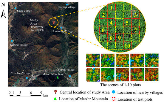
Figure 1.
Location of the study area.
2.2. True-Color Point Cloud Data Acquisition
In this study, a new low-cost integrated UAV image-LiDAR system which consists of DJI Zenmuse LI UAV, an RGB sensor, and a LiDAR sensor was used to acquire true-color point clouds of the study plots. This scanning system not only has the advantage of fast and accurate data acquisition by UAV platform, but also integrates Livox LiDAR, high-precision inertial guidance, a mapping camera, and other modules to attach visible optical images to the synchronously acquired point cloud data and finally output true-color point clouds. The data were collected on 21 July 2022 under good weather conditions with clear sky and no wind. The RGB sensor is a mapping camera with 20 million effective pixels; the LiDAR sensor is a Livox with a repetitive scan mode that provides an oblate field of view (70.4 horizontally and 4.5 vertically). The ground was taken as the baseline, and a relative altitude of 150 m and a flight speed of 8 m/s were set. To ensure sufficient overlap of point cloud data for strip leveling and accuracy of model coloring, the collateral overlap was set to 80%, the sampling frequency was 160 kHz, and the obtained LiDAR data point cloud density was 200 pts/m2. The data coordinate system was WGS-84.
2.3. Methods
Firstly, the obtained true-color point cloud data of the forest stand was preprocessed to eliminate the impacts of noise and ground points. The single tree was then segmented using LiDAR360’s point cloud segmentation tools. Considering the possible loss of the crown point cloud after segmentation, the traditional geometric method and the method based on deep learning were, respectively, used to complete the point cloud, so as to ensure the integrity of the tree point cloud sample and compare the completion performance of different methods. Secondly, the RGB features and LiDAR point cloud features were extracted, respectively, including spectral band, vegetation index, point cloud derived data, and tree structure parameters. Five machine learning classifiers, including RF, SVM, BPNN, QDA, and KNN were used to identify tree species, and the classification results were compared and analyzed. Finally, the classifier with the highest accuracy was selected to rank the importance of all feature indicators, and the impact of different features on the classification results of tree species was discussed through importance analysis. The technical route is shown in Figure 2.
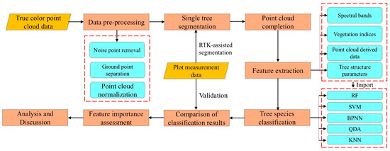
Figure 2.
Technical route. The yellow blocks represent the data used, the pink blocks represent the processing steps, and the blue blocks marked with dotted lines represent the parameters or methods.
2.3.1. Data Pre-Processing and Single Tree Segmentation
Noise points inevitably exist in the original point cloud data due to environmental influences and random error generation. In this study, an isolated point algorithm was used for noise removal based on the LiDAR360 software V3.0 which was provided by Beijing Digital Green Earth Ltd. (Beijing, China) [47,48]. The isolated points can be regarded as independent points that are far away from most other object points. According to the actual distribution of the point cloud data, this study searched and removed the isolated points by setting the number of neighborhood points to 5 and the neighborhood search radius to 10 m, and the final processing results were manually corrected. Meanwhile, the point cloud was divided into ground and non-ground points based on the digital morphological filtering method [49], where the ground points include forest roads, gaps, and open spaces and the non-ground points are mainly vegetation point clouds. The separated point clouds were then normalized to remove the influence of topography, thus better reflecting the true height of the trees.
Single tree segmentation is a prerequisite for extracting the structural parameters of trees and for classifying tree species. The principle is to segment the discrete point clouds into multiple parts, each of which can be treated as a single tree. In this study, the layer stacking algorithm embedded in LiDAR360 software was used to extract individual tree positions from normalized point cloud data. Then, the information of tree locations was used as seed points [50]. Finally, single-tree segmentation was performed based on the normalized point cloud and the corresponding seed points file. The segmented single-tree point cloud data was matched with RTK positioning data from the field investigation. The matching process was conducted based on the following rules: (1) if the segmented crown contains only one single-tree data from the field investigation, the segmentation is considered accurate; (2) if the segmented vector crown does not contain complete single-tree data, it is considered over-segmented and the crown is deleted; (3) if the segmented crown contains multiple trees data, it is considered under-segmented and the segmentation result is retained by manual adjustment to meet subsequent classification requirements [22,51].
2.3.2. Point Cloud Completion
Due to factors such as the environment disturbance, hardware limitations, and occlusion between objects, the data collected by sensors is often incomplete. Point cloud completion aims to generate a complete set of points with the full shape from incomplete- or partial-input point clouds. Similarly, crown overlap between adjacent trees often occurs, which leads to incomplete point clouds after individual tree segmentation. This directly affects the accuracy of feature extraction and species classification. Therefore, this study used both traditional geometric methods and deep learning-based techniques to complete the missing point clouds and compare their results.
Traditional Point Cloud Completion Method
Traditional point cloud completion methods infer the missing parts by identifying geometric patterns in the input point cloud. This approach requires the original point cloud to exhibit a certain level of symmetry and regularity. Based on the crown structure, conifer tree crowns are typically conical in shape [52], with the cross-section resembling a triangle. Similarly, broadleaf tree crowns are mostly hemispherical [53], with the cross-section resembling a semi-ellipse. Therefore, this study proposed the following completion rules based on tree structures:
- (1)
- When distinct trunk points are present in the individual tree point cloud, the trunk is used as both the central and symmetry axis. Then, the existing crown point cloud is rotated and replicated around the trunk to approximate the completion of the missing crown.
- (2)
- When distinct trunk points are absent in the individual tree point cloud, the crown is completed based on the morphological structure of conifer and broadleaf trees, as shown in Figure 3. The colored regions represent the existing crown, while the dashed areas simulate the missing crown, and the combination of the two forms is the complete crown. In the given conifer (broadleaf) tree model, P1 is the highest point in the missing crown point cloud, P2 is the vertex of the complete crown, h is the vertical distance between P1 and P2, and H is the crown height of the missing crown. The Hough transform is used to fit the edge points of the crown to extract the center point O of the tree and the radius D of the fitted circle. Based on the coordinates of point P1 (x1, y1), the distance d between the tree center O and the point P1 in the xoy plane is calculated. Finally, the following calculations can be derived using the theory of similar triangles and the ellipse equation:
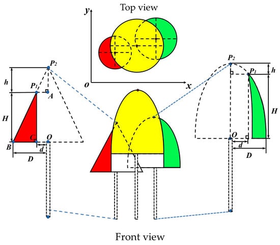 Figure 3. Schematic diagram of tree crown completion. The yellow part represents the trees in the plots. The red and green parts are the data collected after the tree crowns were shaded, and the dashed parts are the simulated actual complete trees. P1 is the highest point in the point cloud of the missing tree crown in the collected data, P2 is the vertex of the actual complete tree crown, H is the crown height, and h is the vertical distance between P1 and P2. O is the center point of the vertical projection plane of the tree crown. d is the distance between the vertical projection of point P1 and O. D is the radius of the fitted circle. A, B, C, are the edge point on the tree crown.
① In the conifer tree model, the projection of point P1 onto the xoy plane is denoted as C. Since ΔAP1P2 and ΔBCP1 are similar triangles, the following condition must be satisfied:
(D − d)/H = d/h.
② In the broadleaf tree model, the crown cross-section is considered as a semi-ellipse. Therefore, point P1, as a point on the ellipse, must satisfy the ellipse equation:
H2/(H + h)2 + d2/D2 = 1.
In the equation, D, d, and H can be obtained through extraction or calculation. Therefore, the value of h determines whether the individual tree crown can be completed. According to existing studies [54,55,56], when h < 0.5 m in the conifer model and h < 0.8 m in the broadleaf tree model, the tree height extraction error is within an acceptable range. And the line connecting points P1 and O in the model can be considered the central axis of the crown. Based on the central axis OP1, the missing crown point cloud is completed by rotating and replicating. Conversely, when the h error is large, it is considered that the vertex position of the individual tree crown cannot be identified. And completing the crown would result in the significant discrepancy from the actual tree structure, which could influence the accuracy of tree species classification. Therefore, the crown point cloud should be discarded.
Point Cloud Completion Method Based on Deep Leaning
In recent years, GANs have been extensively studied. Through the alternating optimization between the generator and discriminator, GANs have significantly improved model training accuracy and efficiency. Inspired by related studies [30,31,32], this study introduced the structure of GAN for tree point cloud completion, as shown in Figure 4.
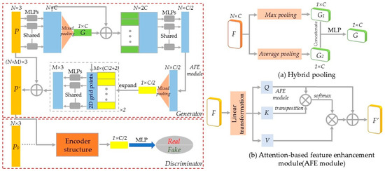
Figure 4.
Point cloud completion network based on GAN. (a) Hybrid pooling. (b) Attention-based feature enhancement (AFE) module.
The generator and discriminator models were constructed based on the structure of GAN. During the training process, the generator attempted to create more realistic data to deceive the discriminator, while the discriminator improved its ability to distinguish between real and generated data, ultimately reaching a dynamic equilibrium. For a given incomplete tree point cloud P, the global features G were extracted using shared MLP and pooling layers. Then, the global and local features were combined to output the encoding vector. In the decoder, 2D grid data and folding operations were used to generate arbitrary point cloud shapes. The combination of P and the generated point cloud produced the final complete tree point cloud P′. To ensure the accuracy of the generated point cloud shape, the discriminator was used to classify whether the input point cloud comes from real or generated data. To enhance feature extraction efficiency and accuracy, two modifications were made to the network: (1) Hybrid pooling module. Traditional dimensionality reduction in features usually employ max pooling, which retains only the maximum value of the point cloud neighborhood, resulting in significant loss of detailed information. Therefore, this study improved the method by using a hybrid pooling module. The input features underwent both max pooling and average pooling, and the resulting two C × 1 feature maps were combined to generate the final point cloud shape features by MLP. (2) Attention-based feature enhancement module. The study used the attention mechanism to calculate the degree of correlation between each point in the input point cloud feature matrix and all other points. The feature of each point was represented as a weighted sum of all features in the point cloud, enabling the network to focus on relevant features and reduce dependence on irrelevant ones.
In the construction of loss function, it is necessary to consider the completion loss of tree point cloud and the adversarial loss of network. Therefore, the overall loss function can be defined as:
In the equation, λ1 and λ2 are weight parameters, Lcom is used as the tree point cloud compensation loss, and the chamfering distance (CD) is used to describe the similarity between the reconstructed point cloud Ycom and the ground truth point cloud Ygt, (x and y are any point in Ycom and Ygt, respectively).
The adversarial loss Ladv is composed of two parts: the discriminant loss of the generated point cloud Yi and the discriminant loss of the input point cloud Xi.
In the equation, D(.) and G(.)are represented as abstract discriminator network and generator network, respectively. S indicates the size of the point cloud dataset.
2.3.3. Feature Extraction
Since the data acquired by the UAV contains both visible band and 3D point cloud information, the extraction of features can be divided into visible band feature extraction and 3D point cloud information feature extraction. The feature extraction of RGB information includes 9 features of mean, standard deviation, and skewness for the red, green, and blue bands, and 8 features of vegetation index selected based on RGB bands calculation [57,58,59,60,61,62,63], including NGRDI, NGBDI, VDVI, RGRI, BGRI, WI, RGBRI, and RGBVI.
Geometric information from LiDAR was mainly related to the structure of the crown [64,65], and LiDAR-intensity features had proven to be meaningful when applied to tree species classification [4]. Therefore, this study divided the LiDAR data into derived data features and single tree structure parameter features based on other research [20,22,66]. The derived data features included the average, minimum, maximum, standard deviation, and variance of strength. The structural parameters were extracted from the single tree parameters for each tree species based on the results of single tree segmentation, including tree height, crown width, crown height, crown projection area, and crown volume. The parameters extracted based on LiDAR were conducted by LiDAR 360 software. A total of 30 features are presented in Table 2, which will be used as input data for machine learning.
Table 2.
Summary of the data features.
2.3.4. Classification Methods
Different machine learning algorithms exhibit different classification performance and comparing machine learning algorithms can help to find a suitable tree classification algorithm. In this study, five classifiers, including RF, SVM, BPNN, QDA, and KNN, were used in Matlab 2019 to realize tree species classification and the best classifier was selected for the subsequent studies.
- (1)
- Random Forest
RF is a popular ensemble learning technique that combines the predictive power of multiple decision trees [67,68]. The core of the RF lies in two types of randomness: random sampling of training data when constructing decision trees, and random selection of features when splitting nodes. In the task of species identification, RF determines the final species label through a majority voting mechanism. Even if the sample size is very small, RF can also generalize it well. In addition, RF also has the characteristics of noise resistance, data tolerance, and not easy to overfit, so as to avoid over learning [69]. The selection of the number of decision trees (n) and the number of leaf nodes (m) is very important in the RF model. When n is too small, the model will show as under fitting. On the contrary, if n is too large, the model will tend to be stable, however, the amount of calculation will increase significantly. Since (N is the candidate feature variable), which should be less than the number of feature variables actually used, multiple tests were conducted by selecting different m values and constructing corresponding regression models in order to obtain the optimal m value with the least error.
- (2)
- Support Vector Machine
SVM is a non-parametric classifier. Its principle is to map the original vector into a higher-dimensional space and create a maximum interval hyperplane in the space, separating the middle hyperplane by the hyperplane on either side to maximize the distance between the two planes [70,71]. When replacing the high-dimensional space with a two-dimensional space, this hyperplane can be viewed as a line. SVM has high generalizability and has a high degree of tolerance for data [72]. However, the tree species classification problems are typically nonlinear and cannot be effectively separated by a simple hyperplane. Therefore, SVM introduces the kernel trick to address this issue, mapping the data into a higher-dimensional space where it becomes linearly separable. In this study, the radial basis function (RBF) with small error and high classification accuracy is selected when building the SVM model. The two important parameters are the kernel parameter g and the penalty coefficient C. The kernel parameter g has impacts on the speed of training and prediction, while the value of penalty coefficient C affects the fitting degree of the model.
- (3)
- Back Propagation Neural Network
BP neural network is a multi-layer feed-forward neural network that can achieve an arbitrary non-linear mapping from input to output and is one of the most widely used neural network models today [73]. It contains an input layer, an output layer, and an implicit layer in between the input and output layers [74]. Furthermore, optimizing the BP NN is crucial for improving the robustness of a model. Commonly used algorithms include Gradient Descent (GD), Adam, and Genetic Algorithm (GA) [75,76,77]. The GD algorithm iteratively updates the parameters, gradually reducing the loss value of the function until reaching a local minimum; the Adam algorithm computes the expected values of gradient momentum and squared gradients to dynamically adjust the learning rate of the parameters, thereby accelerating the convergence process. However, the above two optimization algorithms primarily focus on local optima. In species classification studies, it is more important to consider all samples and features in the dataset to find the optimal classification model. Therefore, this study employs the GA for optimization. This algorithm is a heuristic method that simulates natural selection and genetic mechanisms. It iteratively searches for the optimal solution by initialization, selection, crossover, and mutation steps. In contrast, the population-based search strategy is employed by GA, enabling parallel search for multiple solutions. This effectively prevents them getting trapped in local optima and is better suited for tree species classification tasks.
- (4)
- Quadratic Discriminant Analysis
Discriminant analysis is a classical machine learning method, which belongs to the probability distribution model. QDA is a generalized linear model primarily used to solve classification problems [78]. In species classification, the basic idea of QDA is to apply Bayes’ theorem to establish a quadratic discriminant function for each species. Then, the new samples are assigned to the tree species with the highest discriminant function value. Specifically, QDA assumes that the data for each species follow a Gaussian distribution, and each species is allowed to have its own mean vector and covariance matrix. Therefore, QDA can better capture the nonlinear relationships between species, thereby improving classification performance for nonlinearly separable data [79]. The discriminant function is as follows:
In the equation, represents the discriminant function of the tree category; x represents the input eigenvector; represents the mean vector of the tree category; represents the covariance matrix of the tree category; and represents the prior probability of the tree category.
The QDA algorithm is highly flexible and can adapt to the nonlinear structure of feature data. However, as the data dimensionality increases, the computational complexity of QDA rises significantly, limiting its application in handling large-scale datasets.
- (5)
- K-Nearest Neighbors
KNN is a simple, intuitive, and highly adaptable machine learning algorithm. The principle of the algorithm is based on an assumption: if there are K nearest samples in the feature space of a given sample, and most of these samples belong to a specific category, then the given sample also belongs to that category [80,81]. An important parameter in the KNN algorithm is the choice of K, which directly affects the classification outcome. A small K value may lead to overfitting, while a large K value may lead to underfitting [82]. Therefore, cross-validation is commonly used to determine the optimal K value. In species classification, the KNN algorithm can identify unknown species based on the similarity between different samples. The process involves the following steps: (1) Determine the K nearest samples for classification; (2) Calculate the distance d between the predicted tree sample and each training sample; (3) Compute the maximum distance dmax among the K nearest samples. If dmax < d, the corresponding training sample is recorded. (4) Repeat the above steps until the distances between all predicted tree samples and training samples are calculated and count the frequency of each species among the nearest samples. The species with the highest frequency is assigned as the predicted category of the sample.
The main hyperparameter settings of the above machine learning algorithm are shown in Table 3:
Table 3.
Hyperparameter settings for different machine learning algorithms.
3. Results
3.1. Completion Results of Tree Crown Point Cloud
Point cloud data from the sample site were segmented using LiDAR360 software, resulting in 1011 tree point clouds. According to statistics, 323 trees exhibited varying degrees of point cloud incompleteness, accounting for 31.9%. Therefore, this study selected 688 complete individual tree point clouds, including 130 Pinus koraiensis, 123 Larix gmelinii, 104 Ulmus pumila, 98 Fraxinus mandshurica, 92 Juglans mandshurica, 112 Betula platyphylla, and 29 other tree species. The uniform sampling method was used to extract 10,000 points from the complete tree point clouds as ground truth (GT) data. Then, non-uniform partial sampling of the ground truth data was performed to create point cloud samples with missing crowns. The experiment used both traditional geometric methods and deep learning methods to complete the missing point clouds. The traditional completion algorithm was developed in Matlab R2019b, while the completion algorithm based on the GAN network was implemented using PyTorch 1.11.0. In the hyperparameter settings, λ1 and λ2 were set to 20 and 0.1, respectively; the initial learning rates of the generator and discriminator were both 0.0001; the batch size was 32, and each batch included 200 epochs; and the Adam optimizer was employed for the training process. Moreover, all experiments were conducted on a Dell Precision 7550 workstation equipped with an Intel Core i7 10750H CPU @ 2.4GHz processor (Intel Inc., Santa Clara, CA, USA) and an NVIDIA Quadro RTX 3000 graphics card (6GB GDDR6). The similarity between the completed point clouds generated and the real point clouds was evaluated using the CD and F-scores. The comparison results are shown in Table 4, where the CD values are multiplied by 1000.
Table 4.
Completion results of tree point cloud with different method evaluated by CD×1000 (lower is better) and F-Score@1% (higher is better).
As shown in the Figure 5, the GAN-based method of point cloud completion generated more complete and compact point clouds, with fewer random noise points, and was closer to the ground truth overall. The quantitative results further confirmed the strong completion performance of this network (avgCD = 6.14; avgF1 = 0.85). While the geometric-based completion method partially completed the overall structure of the trees to some extent, the distribution of the completed point clouds lacked regularity, resulting in poor completion of the tree details (avgCD = 10.75; avgF1 = 0.62). From the perspective of tree species, the completion results for coniferous trees, such as Pinus koraiensis and Larix gmelinii, were generally better than those for broadleaf trees, like Ulmus pumila and Juglans mandshurica (avgCDconiferous = 5.32 < avgCDbroadleaf = 6.49, by the GAN-based method). The main reason for this result is that coniferous tree crowns are primarily conical, making them smaller and simpler than the crowns of broadleaf trees. In contrast, broadleaf tree crowns are more complex and variable, which poses challenges to the performance and accuracy of deep learning-based completion methods using adversarial networks.
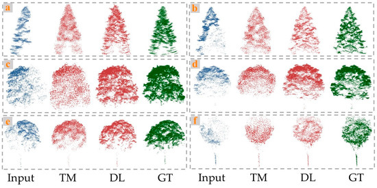
Figure 5.
Visual comparisons on completion of tree point cloud by traditional method (TM) and deep leaning method (DL). (a) Pinus koraiensis, (b) Larix gmelinii, (c) Ulmus pumila, (d) Fraxinus mandshurica, (e) Juglans mandshurica., and (f) Betula platyphylla.
To assess the impact of the improved modules on network performance, the study planned to design ablation experiments. Except for changes made to the hybrid pooling module and the AFE module in the point cloud completion network, the other parts remain unchanged. (1) Model 1: remove the AFE module and replace the hybrid pooling layer with a max pooling layer. (2) Model 2: remove the AFE module and replace the hybrid pooling layer with an average pooling layer. (3) Model 3: retain the AFE module and replace the hybrid pooling layer with a max pooling layer. (4) Model 4: retain the AFE module and replace the hybrid pooling layer with an average pooling layer. The results are shown in Table 5. The results showed that when the hybrid pooling module or AFE module was replaced, the completion performance of the network decreased to varying extents. The main reason was that max pooling and average pooling cannot fully extract the features of interest. For tree point clouds with relatively complex structures, it was essential to enhance feature extraction and representation capabilities. This enhancement directly affected the learning efficiency and generalization ability of the network.
Table 5.
Performance of ablation experiments evaluated by CD × 1000 (lower is better) and F-Score@1% (higher is better).
3.2. Comparison of Classification Results by Different Models
A total of 30 features from 1011 trees, based on the vegetation index calculated by the spectral band and the structural parameters extracted by the LiDAR360 software, were imported into the machine learning classifiers (RF, SVM, BPNN, QDA, and KNN). A total of 70% of the feature data were utilized in training, while the remaining 30% were utilized in testing. Five machine learning algorithms were used to classify both the tree dataset A with incomplete point clouds and the tree dataset B with completed point clouds, respectively. The classification results are shown in Table 6 and Table 7. The classification accuracy of the tree dataset after completion showed a significant improvement, indicating that completing missing point clouds is a necessary step for accurate species classification.
Table 6.
Classifier accuracy of different tree species in the sample plots (data A).
Table 7.
Classifier accuracy of different tree species in the sample plots (data B).
In the classification of dataset B, it can be seen that compared with other classifiers, the classification accuracy of RF was the highest with OA-87.41% and a Kappa coefficient-0.85 while the classification result of QDA was the worst among the five, with a classification accuracy less than 70% and a Kappa coefficient of only 0.66. According to the classification accuracy of different tree species, Pinus koraiensis, Larix gmelinii, and Betula platyphylla showed relatively higher classification accuracy in the five methods, with an average of 84.34%, 85.12%, and 81.42%, respectively, and Fraxinus mandshurica and Juglansl mandshurica did not perform well in classification, only 73.36% and 72.85%. The classification results by RF are illustrated in Figure 6.

Figure 6.
Results of RF-based tree species classification with plots 1–10.
3.3. Feature Importance Evaluation
In this study, the RF classifier showed the best tree species identification, so the 30 feature indices derived from the RGB and LiDAR data were input into the RF classifier. After averaging the importance over several experiments, the features were ranked by importance (Figure 7). Among the RGB features, the blue-light band had a larger contribution ratio to the classification, and vegetation indices such as NGBDI, BGRI, NGRDI, RGBRI, and RGRI had a relatively good performance. With regard to the LiDAR point cloud feature data, the intensity mean value had the highest importance (0.68), and the crown difference, crown mean value, crown area, and crown height ratio in the tree structure features all played a key role in the classification results. In summary, visible features were slightly more important than LiDAR point cloud features. Among the top 10 features in terms of importance, the vegetation indices accounted for 50%, and the rest were LiDAR point cloud features. The tree structure parameters account for 30% of the top 10 features.
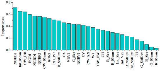
Figure 7.
Overall ranking of feature importance.
To further investigate the selection of feature indices by tree species, the analysis of variance (ANOVA) and least square difference (LSD) were used to distinguish the features with higher overall classification importance (top 10 characteristics of importance), as shown in Table 8 and Table 9. The distribution of the top 10 features in terms of importance by tree species are also represented in a box chart as Figure 8 shows. Based on the statistical results, it can be concluded that both the vegetation index and the tree structure parameters were applicable to distinguish different tree species, indicating that the vegetation index and the tree structure parameters had a high reliability in the classification. When classifying the tree species, the vegetation index was more likely to distinguish Pinus koraiensis from Larix gmelinii, while the LiDAR feature had a better performance in the identification of trees with small tree crowns, especially for Betula platyphylla.
Table 8.
Summary of ANOVA results by features.
Table 9.
Summary of LSD results between the tree species.
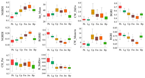
Figure 8.
Distribution of the top 10 features in terms of importance by tree species.
4. Discussion
4.1. Analysis of Point Cloud Completion Algorithm
The creation of high-quality datasets is essential for species classification tasks. During the collection of point clouds in forest plots, equipment limitations and tree occlusions often result in missing data. Therefore, it is crucial to complete low-quality point clouds before performing species classification tasks. This study proposed a feasible solution: a GAN-based deep learning point cloud completion algorithm. When compared with traditional completion methods, the GAN-based completion algorithm demonstrated superior results (avgCD = 6.14; avgF1 = 0.85). The main reason was that the GAN model can automatically adjust parameters through adversarial learning, ultimately generating realistic tree point clouds. This study also improved the network by hybrid pooling and AFE modules, further enhancing the completion performance. Similarly, Zhang et al. [83] proposed ShapeInversion based on the GAN network for unsupervised point cloud completion. It achieved good completion results across all categories in the ShapeNet dataset, with an average CD of 14.9 (scaled by 104). Sarmad et al. [84] were the first to use reinforcement learning agents to control GAN networks, effectively enabling real-time point cloud completion. Experimental results on the ShapeNetCore dataset reported the CD deviation of less than 9% between the reconstructed point clouds and the actual point clouds. Jin et al. [85] proposed an adversarial point cloud completion network based on graph convolution. Experimental results on the PCN dataset showed that the network effectively balanced the extraction of local and global features, alleviating issues of detail loss and uneven distribution in the generated point clouds. It is worth noting that most studies of point cloud completion used public datasets, such as ShapeNet, PCN, and KITTI. These datasets focused primarily on objects with regular shapes, flat surfaces, and symmetric structures, such as furniture, vehicles, and buildings [26,30]. In contrast, tree point clouds have more complex structures, which impose higher performance requirements on completion networks. Additionally, the point cloud completion effect is also related to the tree species. The crown structure of coniferous trees is simple and small, while broadleaf trees have complex and variable crown structures. This means that the completion network is more likely to be affected by random variations when generating broadleaf tree point clouds, which makes the point cloud reconstruction more challenging.
4.2. Comparison of Classification Methods
To identify suitable machine learning algorithms for species classification, this study conducted experiments on RF, SVM, BPNN, QDA, and KNN. The results indicated that RF achieved the highest classification accuracy (OA = 87.41%). In comparison, SVM and BPNN showed varying degrees of accuracy decline when faced with large-scale multi-class tasks, with accuracies of 83.65% and 78.18%, respectively. QDA was sensitive to outliers in feature variables, so it was unsuitable for more complex species classification tasks (OA = 62.06%). The limitation of KNN is that the prediction effect of KNN is poor for a few categories when the number of samples is unbalanced, such as Fraxinus mandshurica (acc = 62.88%) and Juglans mandshurica (acc = 61.30%) in this study. The advantage of RF lies in aggregating the predictions of multiple decision trees, typically providing higher predictive accuracy than the single decision tree. Additionally, RF randomly selects samples and features during the training process, which helps reduce the impact of noise and outliers on model performance, thereby enhancing the robustness of the model [86,87]. Similarly, other scholars found that the RF classifier showed the best performance among different machine learning classifiers. For example, Li et al. [88] compared the classification accuracy of three machine learning methods (RF, SVM, and Decision Tree) on tree species based on Landsat imagery with the addition of topographic features. Their results showed that RF achieved the highest classification accuracy of 83.6%. Li et al. [89] compared the classification accuracy of KNN (K-Nearest Neighbor), SVM, and RF classifiers on shrub species based on UAV-based RGB images and found that the best classification results were obtained using a combination of the optimal variable set and the RF model with an 88.63% overall accuracy. Li et al. [17] combined spectral features, vegetation indices, LiDAR variables, and tree crown characteristics to conduct species classification research, which reported that the classification accuracy of RF was approximately 4.5% higher than that of BPNN. On the other hand, research by Zhong [90] and Quan [91] also demonstrated the interpretability of RF in species classification. RF can assess the importance of features during the prediction process, which helps identify the key features that contribute to species classification, thereby guiding subsequent feature selection and model optimization. The above conclusions were consistent with those obtained in this study.
4.3. Impact of Features on Classification
Vegetation indices, as a measure of surface vegetation cover and plant growth, have been widely used in tree species classification [92,93]. Among the top 10 features in terms of importance, vegetation indices accounted for 50%. However, tree structure parameters also contributed highly to the classification, which accounted for 30% of the top 10 features, indicating that point cloud data features such as tree structure parameters can be used as an important basis for tree species classification. Similarly, Deng et al. [20] showed that the addition of airborne LiDAR-based features such as crown convex hull area, crown convex hull volume, and shape index to the spectral features contributed to the tree species classification results, compared to those using only spectral data. Wan et al. [12] demonstrated that one of the most helpful pieces of information for tree species classification came from LiDAR data, mainly due to the fact that the profile curves generated from LiDAR data contained rich information on stand structure, which was effective in differentiating tree species. Therefore, high-precision 3D structural features of trees extracted by LiDAR played an important role in tree species classification tasks.
In this study, features with higher importance (top 10 characteristics of importance) were selected for ANOVA and LSD analysis in combination with tree species, based on an overall ranking of the importance of the feature classification. The vegetation indices NGBDI, BGRI, and RGBRI, and the standard deviation B_StdDev were more helpful in distinguishing conifers from broad-leaved trees. All of these spectral features were contained in the blue band, indicating that the blue band had an important role in tree species classification. Canopy-related features (CW_Dif, CW_Mean, CH_Per) are associated with tree morphology, which also performed well in tree species classification. Pinus koraiensis and Larix gmelinii had the smallest crowns, followed by Betula platyphylla. Fraxinus mandshurica and Juglans mandshurica were generally large in tree crown, while Ulmus pumila had the largest crowns. Thus, the crown structure parameters were crucial for the classification of tree species. In addition, intensity information was also an important factor in classification. As a measure of pulse-echo size, intensity can reflect the spectral reflectance of the scanned object to some extent. Therefore, intensity values have a greater potential for classification. Among the species, Pinus koraiensis achieved the highest classification accuracy of 93.75%. The classification accuracy of Ulmus pumila, Fraxinus mandshurica, and Juglans mandshurica was relatively poor, with an average of 82.52%, due to the fact that the three tree species were similar in spectral band values and tree structure.
4.4. Limitations and Future Research
It should be noted that there are also some limitations in this study. Six dominant tree species with a relatively small sample size in the study area of natural secondary forest were selected for tree species classification due to the constraints of the sample plots. More species with relatively larger sample sizes under different forest types and site conditions should also be analyzed in the future research to test the robustness of the results. In terms of the algorithm, the GAN-based method of tree point cloud completion has achieved promising results. However, the effectiveness and advanced nature of the method used in the network structure design still require further validation. The classification methods used in this study belong to common machine learning algorithms. In the future research, the other machine learning models can also be applied in order to increase the robustness of the results. In addition, deep learning is also well-suited for handling classification problems, such as PointNet, PointNet++, and PointCNN. Deep learning has powerful capabilities of feature extraction, making it highly effective in handling high-dimensional data with complex points. However, deep learning typically adopts an end-to-end learning approach, directly mapping input data to output tasks. This approach makes the decision-making process within the model difficult to intuitively understand. Moreover, the interactions between the large number of neurons in the network form complex nonlinear transformations, enabling the model to capture high-level abstract features in the data. But it also makes the model’s behavior difficult to predict and explain. In the species classification task of this study, machine learning algorithms can explain the relationship between classification results and feature parameters, and identify the sensitive features for the classification of specific tree species. Therefore, the advantages of machine learning and deep learning will be combined to conduct more systematic and in-depth research on high-precision tree species classification in future work. Finally, there is still much room for the development of near-ground UAV platforms in forest inventory, so as to improve the accuracy and efficiency of tree species identification via multi-source UAV remote sensing data.
5. Conclusions
In this study, the single tree was segmented based on true-color point cloud, and the missing tree point cloud was completed based on a deep learning network. Then, different machine learning algorithms in combination with the feature indicators extracted from RGB data and LiDAR point clouds were used to construct models for tree species classification. With the optimal classifier, the feature indicators were ranked according to their importance. The main findings are as follows:
- (1)
- The GAN-based method of point cloud completion was proposed and introduce hybrid pooling module and AFE module to improve the network structure. This method finally achieved a good completion effect (avgCD = 6.14; avgF1 = 0.85). By comparing the classification accuracy of incomplete and completed trees, we demonstrated that the completion of missing point clouds was necessary. This method makes it possible to extract features from more detected single trees and lays a foundation for subsequent tree species classification.
- (2)
- In the classification of completed trees, the RF classifier showed the best performance with a limited number of training samples (OA = 87.41%) compared with the classification model constructed by other machine learning algorithms. The classification accuracy of coniferous trees including Pinus koraiensis and Larix gmelinii was higher, with the classification accuracy of more than 90%. Among the broad-leaved trees, the classification accuracy of Fraxinus mandshurica and Juglans mandshurica was poorer, with an average classification accuracy of about 80%.
- (3)
- The overall importance of RGB features was slightly greater than that of LiDAR point cloud features. The vegetation indices including VDVI, RGBRI, RGRI, NGRDI, and NGBDI and the intensity mean and skewness of LiDAR-derived data together with the tree structure features including crown area, crown width mean, and crown height, had a greater contribution to the tree species classification, which proved that the LiDAR point cloud can be used as an important data support for tree species classification. In addition, different feature indicators had different classification effects on different tree species. Both the vegetation indices and the tree structure parameters performed better for the identification of Pinus koraiensis, while the intensity features were more discriminative for Betula platyphyll.
Author Contributions
Conceptualization, H.L.; methodology, H.L.; software, H.L. and G.X.; validation, H.L., H.Z., G.X. and P.Z.; formal analysis, H.L. and P.Z.; investigation, H.L. and H.Z.; resources, H.L. and H.Z.; data curation, H.L.; writing—original draft preparation, H.L.; writing—review and editing, H.L., G.X. and P.Z.; visualization, H.L.; supervision, G.X. and P.Z.; project administration, H.Z.; funding acquisition, H.Z. All authors have read and agreed to the published version of the manuscript.
Funding
This research was funded by the Fundamental Research Funds for the Central Universities (Grant number: 2572021AW49), and the Innovation Foundation for Doctoral Program of Forestry Engineering of Northeast Forestry University (Grant number: LYGC202114).
Data Availability Statement
The original contributions presented in this study are included in the article. Further inquiries can be directed to the corresponding author.
Acknowledgments
We gratefully acknowledge the assistance of Heilongjiang Jingzhen Science & Technology Development Co., Ltd. in preparing the UAV laser scanning point cloud data. We also thank Lin and Wu for their guidance on the manuscript.
Conflicts of Interest
The authors declare no conflicts of interest.
References
- Li, R.N.; Ou, G.L.; Dai, Q.L.; Xu, W.H.; Wang, L.G. Forest Types Classification of Shangri-La based on Google Earth Engine and Landsat Time-series Data. J. Southwest For. Univ. (Nat. Sci.) 2020, 40, 115–125. [Google Scholar]
- Cardinale, B.J.; Duffy, J.E.; Gonzalez, A.; Hooper, D.U.; Perrings, C.; Venail, P.; Narwani, A.; Mace, G.M.; Tilman, D.; Wardle, D.A.; et al. Biodiversity Loss and Its Impact on Humanity. Nature 2012, 486, 59–67. [Google Scholar] [CrossRef] [PubMed]
- Pan, Y.; Birdsey, R.A.; Fang, J.; Houghton, R.; Kauppi, P.E.; Kurz, W.A.; Phillips, O.L.; Shvidenko, A.; Lewis, S.L.; Canadell, J.G.; et al. A Large and Persistent Carbon Sink in the World’s Forests. Science 2011, 333, 988–993. [Google Scholar] [CrossRef] [PubMed]
- Fassnacht, F.E.; Latifi, H.; Stereńczak, K.; Modzelewska, A.; Lefsky, M.; Waser, L.T.; Straub, C.; Ghosh, A. Review of Studies on Tree Species Classification from Remotely Sensed Data. Remote Sens. Environ. 2016, 186, 64–87. [Google Scholar] [CrossRef]
- Yang, H.B.; Zhao, J.; Lan, Y.B.; Lu, L.Q.; Li, Z.M. Fraction Vegetation Cover Extraction of Winter Wheat based on RGB Image Obtained by UAV. Int. J. Precis. Agric. Aviat. 2019, 2, 54–61. [Google Scholar] [CrossRef]
- Du, X.Y.; Wan, L.; Cen, H.Y.; Chen, S.B.; Zhu, J.P.; Wang, H.Y.; He, Y. Multi-temporal Monitoring of Leaf Area Index of Rice under Different Nitrogen Treatments Using UAV Images. Int. J. Precis. Agric. Aviat. 2020, 3, 7–12. [Google Scholar] [CrossRef]
- Zhou, X.C.; Zheng, L.; Huang, H.Y. Classification of Forest Stand based on Multi-feature Optimization of UAV Visible Light Remote Sensing. Sci. Silvae Sin. 2021, 57, 24–36. [Google Scholar]
- Cao, K.L.; Zhang, X.L. An Improved Res-UNet Model for Tree Species Classification Using Airborne High-resolution Images. Remote Sens. 2020, 12, 1128. [Google Scholar] [CrossRef]
- Cao, J.J.; Leng, W.C.; Liu, K.; Liu, L.; He, Z.; Zhu, Y.H. Object-based Mangrove Species Classification Using Unmanned Aerial Vehicle Hyperspectral Images and Digital Surface Models. Remote Sens. 2018, 10, 89. [Google Scholar] [CrossRef]
- Dalponte, M.; Bruzzone, L.; Gianelle, D. Fusion of Hyperspectral and LIDAR Remote Sensing Data for Classification Forest Areas. IEEE Trans. Geosci. Remote Sens. 2008, 46, 1416–1427. [Google Scholar] [CrossRef]
- Jones, T.G.; Coops, N.C.; Sharma, T. Assessing the Utility of Airborne Hyperspectral and LiDAR Data for Species Distribution Mapping in the Coastal Pacific Northwest, Canada. Remote Sens. Environ. 2010, 114, 2841–2852. [Google Scholar] [CrossRef]
- Wan, H.M.; Tang, Y.W.; Jing, L.H.; Li, H.; Qiu, F.; Wu, W.J. Tree Species Classification of Forest Stands Using Multisource Remote Sensing Data. Remote Sens. 2021, 13, 144. [Google Scholar] [CrossRef]
- Zhao, Q.H.; Jia, S.H.; Li, Y. Hyperspectral Remote Sensing Image Classification based on Tighter Random Projection with Minimal Intra-class Variance Algorithm. Pattern Recognit. 2021, 111, 107635. [Google Scholar] [CrossRef]
- Wallace, L.; Lucieer, A.; Watson, C.; Turner, D. Development of a UAV-LiDAR System with Application to Forest Inventory. Remote Sens. 2012, 4, 1519–1543. [Google Scholar] [CrossRef]
- Wallace, L.; Musk, R.; Lucieer, A. An Assessment of the Repeatability of Automatic Forest Inventory Metrics Derived from UAV-borne Laser Scanning Data. IEEE Trans. Geosci. Remote Sens. 2014, 52, 7160–7169. [Google Scholar] [CrossRef]
- Liu, Q.W.; Li, S.M.; Li, Z.Y.; Fu, L.Y.; Hu, K.L. Review on the Applications of UAV-based LiDAR and Photogrammetry in Forestry. Sci. Silvae Sin. 2017, 53, 134–148. [Google Scholar]
- Li, J.; Li, M.Z.; Quan, Y.; Wang, B.; Mo, Z.K. Tree Species Classification Using UAV-LiDAR with Hyperspectral Data. J. Northeast For. Univ. 2022, 50, 63–69. [Google Scholar]
- Wang, Y.T.; Wang, J.; Chang, S.P.; Sun, L.; An, L.K.; Chen, Y.H.; Xu, J.Q. Classification of Street Tree Species Using UAV Tilt Photogrammetry. Remote Sens. 2021, 13, 216–222. [Google Scholar] [CrossRef]
- Liu, H.R.; Fan, W.W.; Xu, Y.S.; Lin, W.S. Research Progress in Forest Information Extraction based on Multi-source Data Collaboration Operation. World For. Res. 2020, 33, 33–37. [Google Scholar]
- Deng, S.; Katoh, M.; Yu, X.; Hyyppä, J.; Gao, T. Comparison of Tree Species Classifications at the Individual Tree Level by Combining ALS Data and RGB Images Using Different Algorithms. Remote Sens. 2016, 8, 1034. [Google Scholar] [CrossRef]
- Xu, Z.Y.; Chen, Q.; Chen, Y.F. Tree Species Recognition based on Unmanned Aerial Vehicle Image with LiDAR Individual Tree Segmentation Aided. Trans. Chin. Soc. Agric. Mach. 2022, 53, 197–205. [Google Scholar]
- Li, H.Y.; Zhang, C.; Chen, Q.; Wang, J.; Peng, X.; Xu, Z.Y.; Liu, H.D.; Bai, M.X.; Chen, Y.F. Single Tree Species Identification based on Visible Light and LiDAR Data of UAV. J. Southwest For. Univ. (Nat. Sci. ) 2021, 41, 105–113. [Google Scholar]
- Matsuki, T.; Yokoya, N.; Iwasaki, A. Hyperspectral Tree Species Classification of Japanese Complex Mixed Forest with the Aid of LiDAR Data. IEEE J. Sel. Top. Appl. Earth Obs. Remote Sens. 2015, 8, 2177–2187. [Google Scholar] [CrossRef]
- Alonzo, M.; Bookhagen, B.; Roberts, D.A. Urban Tree Species Mapping Using Hyperspectral and Lidar Data Fusion. Remote Sens. Environ. 2014, 148, 70–83. [Google Scholar] [CrossRef]
- Dalponte, M.; Frizzera, L.; Gianelle, D. Individual Tree Crown Delineation and Tree Species Classification with Hyperspectral and LiDAR Data. PeerJ 2019, 6, e6227. [Google Scholar] [CrossRef]
- You, L.; Sun, Y.A.; Chang, X.S.; Du, L.M. Tree Point Cloud Completion Network based on Attention Mechanism. J. Comput.-Aided Des. Comput. Graph. 2024, 5, 1–10. [Google Scholar]
- Pauly, M.; Mitra, N.J.; Wallner, J.; Pottmann, H.; Guibas, L.J. Discovering Structural Regularity in 3D Geometry. ACM Trans. Graph. 2008, 27, 43. [Google Scholar] [CrossRef]
- Zheng, Q.; Sharf, A.; Wan, G.; Li, Y.; Mitra, N.J.; Cohen-Or, D.; Chen, B. Non-local Scan Consolidation for 3D Urban Scenes. ACM Trans. Graph. 2010, 29, 1–9. [Google Scholar]
- Chen, J.W.; Zhao, L.L.; Ren, L.C.; Sun, Z.Q.; Zhang, X.F.; Ma, S.W. Deep Learning-based Quality Enhancement for 3D Point Clouds: A survey. J. Image Graph. 2023, 28, 3295–3319. [Google Scholar]
- Yuan, W.; Khot, T.; Held, D.; Mertz, C.; Hebert, M. PCN: Point Completion Network. In Proceedings of the 2018 International Conference on 3D Vision (3DV), Verona, Italy, 5–8 September 2018; IEEE: Piscataway, NJ, USA, 2018; pp. 728–737. [Google Scholar]
- Huang, Z.; Yu, Y.; Xu, J.; Ni, F.; Le, X. PF-net: Point Fractal Network for 3D Point Cloud Completion. In Proceedings of the IEEE/CVF Conference on Computer Vision and Pattern Recognition, Seattle, WA, USA, 14–19 June 2020; pp. 7662–7670. [Google Scholar]
- Wang, X.; Ang, M.H.; Lee, G.H. Cascaded Refinement Network for Point Cloud Completion. In Proceedings of the IEEE/CVF Conference on Computer Vision and Pattern Recognition, Seattle, WA, USA, 14–19 June 2020; pp. 790–799. [Google Scholar]
- Kim, S.; Hinckley, T.; Briggs, D. Classifying Individual Tree Genera Using Stepwise Cluster Analysis based on Height and Intensity Metrics Derived from Airborne Laser Scanner Data. Remote Sens. Environ. 2011, 115, 3329–3342. [Google Scholar] [CrossRef]
- Marrs, J.; Ni-Meister, W. Machine Learning Techniques for Tree Species Classification Using Co-Registered LiDAR and Hyperspectral Data. Remote Sens. 2019, 11, 819. [Google Scholar] [CrossRef]
- Jiang, Y.F.; Qi, J.G.; Chen, B.W.; Yan, M.; Huang, L.J.; Zhang, L. Classification of Mangrove Species with UAV Hyperspectral Imagery and Machine Learning Methods. Remote Sens. Technol. Appl. 2021, 36, 1416–1424. [Google Scholar]
- Huang, C.; Davis, L.S.; Townshend, J.R.G. An Assessment of Support Vector Machines for Land Cover Classification. Int. J. Remote Sens. 2002, 23, 725–749. [Google Scholar] [CrossRef]
- Duro, D.C.; Franklin, S.E.; Dubé, M.G. A Comparison of Pixel-based and Object-based Image Analysis with Selected Machine Learning Algorithms for the Classification of Agricultural Landscapes Using Spot-5 HRG Imagery. Remote Sens. Environ. 2012, 118, 259–272. [Google Scholar] [CrossRef]
- Ba, A.; Laslier, M.; Dufour, S.; Hubert-Moy, L. Riparian Trees Genera Identification based on Leaf-on/leaf-off Airborne Laser Scanner Data and Machine Learning Classifiers in Northern France. Int. J. Remote Sens. 2020, 41, 1645–1667. [Google Scholar] [CrossRef]
- Franklin, S.E.; Ahmed, O.S. Deciduous Tree Species Classification Using Object-based Analysis and Machine Learning with Unmanned Aerial Vehicle Multispectral Data. Int. J. Remote Sens. 2018, 39, 5236–5245. [Google Scholar] [CrossRef]
- Plaza, A.; Benediktsson, J.A.; Boardman, J.W.; Brazile, J.; Bruzzone, L.; Camps-Valls, G.; Chanussot, J.; Fauvel, M.; Gamba, P.; Gualtieri, A.; et al. Recent Advances in Techniques for Hyperspectral Image Processing. Remote Sens. Environ. 2009, 113, S110–S122. [Google Scholar] [CrossRef]
- Dalponte, M.; Bruzzone, L.; Vescovo, L.; Gianelle, D. The Role of Spectral Resolution and Classifier Complexity in the Analysis of Hyperspectral Images of Forest Areas. Remote Sens. Environ. 2009, 113, 2345–2355. [Google Scholar] [CrossRef]
- Dalponte, M.; Ørka, H.O.; Gobakken, T.; Gianelle, D.; Næsset, E. Tree Species Classification in Boreal Forests with Hyperspectral Data. IEEE Trans. Geosci. Remote Sens. 2012, 51, 2632–2645. [Google Scholar] [CrossRef]
- Zhao, Y.H.; Zhang, D.L.; Zhen, Z. Individual Tree Species Classification based on Nonparametric Classification Algorithms and Multi-source Remote Sensing Data. J. Nanjing For. Univ. (Nat. Sci. Ed.) 2019, 43, 103–112. [Google Scholar]
- Shi, Y.; Skidmore, A.K.; Wang, T.; Holzwarth, S.; Heiden, U.; Pinnel, N.; Zhu, X.; Heurich, M. Tree Species Classification Using Plant Functional Traits from LiDAR and Hyperspectral Data. Int. J. Appl. Earth Obs. Geoinf. 2018, 73, 207–219. [Google Scholar] [CrossRef]
- Sun, Y.X.; Liu, Z.G.; Dong, L.B. Spatial Point Patterns and Their Association Dynamics of Forest Landscapes in Maoershan region Northeast China between 1983 and 2016. Chin. J. Appl. Ecol. 2018, 29, 2601–2614. [Google Scholar]
- Wei, H.Y.; Zhang, Y.F.; Dong, L.B.; Liu, Z.G.; Chen, Y. Comprehensive Evaluation of Spatial Structure State for the Main Forest Types in Maoershan Mountain. J. Cent. South Univ. For. Technol. 2021, 41, 131–139. [Google Scholar]
- Angiulli, F.; Basta, S.; Pizzuti, C. Distance-based Detection and Prediction of Outliers. IEEE Trans. Knowl. Data Eng. 2005, 18, 145–160. [Google Scholar] [CrossRef]
- Angiulli, F.; Basta, S.; Lodi, S.; Sartori, C. Distributed Strategies for Mining Outliers in Large Data Sets. IEEE Trans. Knowl. Data Eng. 2012, 25, 1520–1532. [Google Scholar] [CrossRef]
- Wu, J. Research on Feature Extraction of Single Wood from Laser Point Cloud for Tending and Harvesting in Forest. Doctoral Dissertation, Beijing Forestry University, Beijing, China, 2021. [Google Scholar]
- Pu, Y.; Xu, D.; Wang, H.; Li, X.; Xu, X. A New Strategy for Individual Tree Detection and Segmentation from Leaf-on and Leaf-off UAV-LiDAR Point Clouds based on Automatic Detection of Seed Points. Remote Sens. 2023, 15, 1619. [Google Scholar] [CrossRef]
- Li, D.; Zhang, J.J.; Zhao, M.X. Extraction of Stand Factors in UAV Image based on FCM and Watershed Algorithm. Sci. Silvae Sin. 2019, 55, 180–187. [Google Scholar]
- Wang, S.T.; Geng, J.; Tu, L.L.; Yin, G.F. Influences of Semiellipsoid-shaped Crown on Gap Fraction and Clumping Index. Natl. Remote Sens. Bull. 2021, 25, 2103–2115. [Google Scholar] [CrossRef]
- Power, H.; Lemay, V.; Berninger, F.; Sattler, D.; Kneeshaw, D. Differences in Crown Characteristics Between Black (Picea mariana) and White Spruce (Picea glauca). Can. J. For. Res. 2012, 42, 1733–1743. [Google Scholar] [CrossRef]
- Cabo, C.; Ordóñez, C.; López-Sánchez, C.A.; Armesto, J. Automatic Dendrometry: Tree Detection, Tree Height and Diameter Estimation Using Terrestrial Laser Scanning. Int. J. Appl. Earth Obs. Geoinf. 2018, 69, 164–174. [Google Scholar] [CrossRef]
- Huang, Z.X. Extraction of DBH and Height Based on Backpack LiDAR Point Cloud Data. Ph.D. Thesis, Northeast Forestry University, Harbin, China, 2021. [Google Scholar]
- Zhao, Y.H.; Yang, H.C.; Zhen, Z. Tree Height Estimations for Different Forest Canopies in Natural Secondary Forests based on ULS, TLS and Ultrasonic Altimeter Systems. J. Nanjing For. Univ. (Nat. Sci. Ed.) 2021, 45, 23–32. [Google Scholar]
- Torres-Sanchez, J.; Pena, J.M.; de Castro, A.I.; Lopez-Granados, F. Multi-temporal Mapping of the Vegetation Fraction in Early-Season Wheat Fields Using Images from UAV. Comput. Electron. Agric. 2014, 103, 104–113. [Google Scholar] [CrossRef]
- Du, M.M.; Noguchi, N. Monitoring of Wheat Growth Status and Mapping of Wheat Yield’s Within-field Spatial Variations Using Color Images Acquired from UAV-camera System. Remote Sens. 2017, 9, 289. [Google Scholar] [CrossRef]
- Wan, L.; Li, Y.J.; Cen, H.Y.; Zhu, J.P.; Yin, W.X.; Wu, W.K.; Zhu, H.Y.; Sun, D.W.; Zhou, W.J.; He, Y. Combining UAV-based Vegetation Indices and Image Classification to Estimate Flower Number in Oilseed Rape. Remote Sens. 2018, 10, 1484. [Google Scholar] [CrossRef]
- Calderon, R.; Navas-Cortes, J.A.; Lucena, C.; Zarco-Tejada, P.J. High-resolution Airborne Hyperspectral and Thermal Imagery for Early, Detection of Verticillium Wilt of Olive Using Fluorescence, Temperature and Narrow-band Spectral Indices. Remote Sens. Environ. 2013, 139, 231–245. [Google Scholar] [CrossRef]
- Woebbecke, D.M.; Meyer, G.E.; Vonbargen, K.; Mortensen, D.A. Color Indexes for Weed Identification Under Various Soil, Residue, and Lighting Conditions. Trans. ASAE 1995, 38, 259–269. [Google Scholar] [CrossRef]
- Xie, B.; Yang, W.N.; Wang, F. A New Estimate Method for Fractional Vegetation Cover based on UAV Visual Light Spectrum. Sci. Surv. Mapp. 2020, 45, 72–77. [Google Scholar]
- Bendig, J.; Yu, K.; Aasen, H.; Bolten, A.; Bennertz, S.; Broscheit, J.; Gnyp, M.L.; Bareth, G. Combining UAV-based Plant Height from Crop Surface Models, Visible, and Near Infrared Vegetation Indices for Biomass Monitoring in Barley. Int. J. Appl. Earth Obs. Geoinf. 2015, 39, 79–87. [Google Scholar] [CrossRef]
- Riaño, D.; Chuvieco, E.; Condés, S.; González-Matesanz, J.; Ustin, S.L. Generation of Crown Bulk Density for Pinus sylvestris L. from LiDAR. Remote Sens. Environ. 2004, 92, 345–352. [Google Scholar] [CrossRef]
- Coops, N.C.; Hilker, T.; Wulder, M.A.; St-Onge, B.; Newnham, G.; Siggins, A.; Trofymow, J.A. Estimating Canopy Structure of Doulgas-fir Forest Stands from Discrete-return LiDAR. Trees 2007, 21, 295–310. [Google Scholar] [CrossRef]
- Zhou, R.; Yang, C.; Li, E.; Cai, X.; Yang, J.; Xia, Y. Object-based Wetland Vegetation Classification Using Multi-feature Selection of Unoccupied Aerial Vehicle RGB Imagery. Remote Sens. 2021, 13, 4910. [Google Scholar] [CrossRef]
- Belgiu, M.; Drăgu, L. Random Forest in Remote Sensing: A Review of Applications and Future Directions. ISPRS J. Photogramm. Remote Sens. 2016, 114, 24–31. [Google Scholar] [CrossRef]
- Pu, R.L.; Landry, S.; Yu, Q.Y. Assessing the Potential of Multi-seasonal High Resolution Pleiades Satellite Imagery for Mapping Urban Tree Species. Int. J. Appl. Earth Obs. Geoinf. 2018, 71, 144–158. [Google Scholar]
- Genuer, R.; Poggi, J.M.; Tuleau-Malot, C. Variable Selection Using Random Forests. Pattern Recognit. Lett. 2010, 31, 2225–2236. [Google Scholar] [CrossRef]
- Torabzadeh, H.; Leiterer, R.; Hueni, A.; Schaepman, M.E.; Morsdorf, F. Tree Species Classification in a Temperate Mixed Forest Using a Combination of Imaging Spectroscopy and Airborne Laser Scanning. Agric. For. Meteorol. 2019, 279, 107744. [Google Scholar] [CrossRef]
- Colgan, M.S.; Baldeck, C.A.; Féret, J.B.; Asner, G.P. Mapping Savanna Tree Species at Ecosystem Scales Using Support Vector Machine Classification and BRDF Correction on Airborne Hyperspectral and LiDAR Data. Remote Sens. 2012, 4, 3462–3480. [Google Scholar] [CrossRef]
- Michałowska, M.; Rapiński, J. A Review of Tree Species Classification based on Airborne LiDAR Data and Applied Classifiers. Remote Sens. 2021, 13, 353. [Google Scholar] [CrossRef]
- Li, B.; Jing, Q. Improved Convolutional Neural Network for Tree Species Recognition. For. Eng. 2021, 37, 75–81. [Google Scholar]
- Lu, Y.H. Plastic Classification Research by LIBS Combined with GA-BP-NN and GA-SVM. Laser Infrared 2022, 52, 273–279. [Google Scholar]
- Liu, C.; Ding, W.; Li, Z.; Yang, C. Prediction of High-speed Grinding Temperature of Titanium Matrix Composites Using BP Neural Network based on PSO Algorithm. Int. J. Adv. Manuf. Technol. 2017, 89, 2277–2285. [Google Scholar] [CrossRef]
- Dong, Z.; Xu, W.; Xu, J.; Zhuang, H. Application of Adam-BP Neural Network in Leveling Fitting. IOP Conf. Ser. Earth Environ. Sci. 2019, 310, 022036. [Google Scholar] [CrossRef]
- Zhang, F.; Zhang, X.; Chen, L.; Sun, L.; Zhan, W. Optimized Neural Network for Binocular Camera Calibration Using Improved Genetic Algorithm. China Mech. Eng. 2021, 32, 1423–1431. [Google Scholar]
- Tharwat, A. Linear vs. Quadratic Discriminant Analysis Classifier: A Tutorial. Int. J. Appl. Pattern Recognit. 2016, 3, 145–180. [Google Scholar] [CrossRef]
- Qin, Y. A Review of Quadratic Discriminant Analysis for High-dimensional Data. Wiley Interdiscip. Rev. Comput. Stat. 2018, 10, e1434. [Google Scholar] [CrossRef]
- Nevalainen, O.; Honkavaara, E.; Tuominen, S.; Viljanen, N.; Hakala, T.; Yu, X.; Hyyppä, J.; Saari, H.; Pölönen, I.; Imai, N.N.; et al. Individual Tree Detection and Classification with UAV-Based Photogrammetric Point Clouds and Hyperspectral Imaging. Remote Sens. 2017, 9, 185. [Google Scholar] [CrossRef]
- Jiang, F.; Smith, A.R.; Kutia, M.; Wang, G.; Liu, H.; Sun, H. A Modified KNN Method for Mapping the Leaf Area Index in Arid and Semi-Arid Areas of China. Remote Sens. 2020, 12, 1884. [Google Scholar] [CrossRef]
- Pacheco, A.d.P.; Junior, J.A.d.S.; Ruiz-Armenteros, A.M.; Henriques, R.F.F. Assessment of k-Nearest Neighbor and Random Forest Classifiers for Mapping Forest Fire Areas in Central Portugal Using Landsat-8, Sentinel-2, and Terra Imagery. Remote Sens. 2021, 13, 1345. [Google Scholar] [CrossRef]
- Zhang, J.; Chen, X.; Cai, Z.; Pan, L.; Zhao, H.; Yi, S.; Yeo, C.K.; Dai, B.; Loy, C.C. Unsupervised 3D Shape Completion Through GAN Inversion. In Proceedings of the IEEE/CVF Conference on Computer Vision and Pattern Recognition, Nashville, TN, USA, 19–25 June 2021; pp. 1768–1777. [Google Scholar]
- Sarmad, M.; Lee, H.J.; Kim, Y.M. RL-GAN-Net: A Reinforcement Learning Agent Controlled GAN Network for Real-time Point Cloud Shape Completion. In Proceedings of the IEEE/CVF Conference on Computer Vision and Pattern Recognition, Long Beach, CA, USA, 16–20 June 2019; pp. 5898–5907. [Google Scholar]
- Jin, S.C. Research on Image Inpainting and Point Cloud Completion Based on Generative Adversarial Network. Master’s Thesis, Dalian Jiaotong University, Dalian, China, 2024. [Google Scholar]
- Karlson, M.; Ostwald, M.; Reese, H.; Bazié, H.R.; Tankoano, B. Assessing the Potential of Multi-Seasonal WorldView-2 imagery for Mapping West African Agroforestry Tree Species. Int. J. Appl. Earth Obs. Geoinf. 2016, 50, 80–88. [Google Scholar] [CrossRef]
- Ghosh, A.; Fassnacht, F.E.; Joshi, P.K.; Koch, B. A Framework for Mapping Tree Species Combining Hyperspectral and LiDAR Data: Role of selected classifiers and sensor across three spatial scales. Int. J. Appl. Earth Obs. Geoinf. 2014, 26, 49–63. [Google Scholar] [CrossRef]
- Li, M.; Im, J.; Beier, C. Machine Learning Approaches for Forest Classification and Change Analysis Using Multi-temporal Landsat TM Images Over Huntington Wildlife Forest. GIScience Remote Sens. 2013, 50, 361–384. [Google Scholar] [CrossRef]
- Li, Z.; Ding, J.; Zhang, H.; Feng, Y.M. Classifying Individual Shrub Species in UAV Images-a Case Study of the Gobi Region of Northwest China. Remote Sens. 2021, 13, 4995. [Google Scholar] [CrossRef]
- Zhong, H.; Lin, W.; Liu, H.; Ma, N.; Liu, K.; Cao, R.; Wang, T.; Ren, Z. Identification of Tree Species based on the Fusion of UAV Hyperspectral Image and LiDAR Data in a Coniferous and Broad-leaved Mixed Forest in Northeast China. Front. Plant Sci. 2022, 13, 964769. [Google Scholar] [CrossRef]
- Quan, Y. Mapping Tree Species and Forest Types in a Typical Natural Secondary Forest by Fusing UAV-borne LiDAR and Hyperspectral features. Ph.D. Thesis, Northeast Forestry University, Harbin, China, 2023. [Google Scholar]
- Sabat-Tomala, A.; Raczko, E.; Zagajewski, B. Comparison of Support Vector Machine and Random Forest Algorithms for Invasive and Expansive Species Classification Using Airborne Hyperspectral Data. Remote Sens. 2020, 12, 516. [Google Scholar] [CrossRef]
- Zagajewski, B.; Kluczek, M.; Raczko, E.; Njegovec, A.; Dabija, A.; Kycko, M. Comparison of Random Forest, Support vector machines, and Neural Networks for Post-disaster Forest Species Mapping of the Krkonoše/Karkonosze Transboundary Biosphere Reserve. Remote Sens. 2021, 13, 2581. [Google Scholar] [CrossRef]
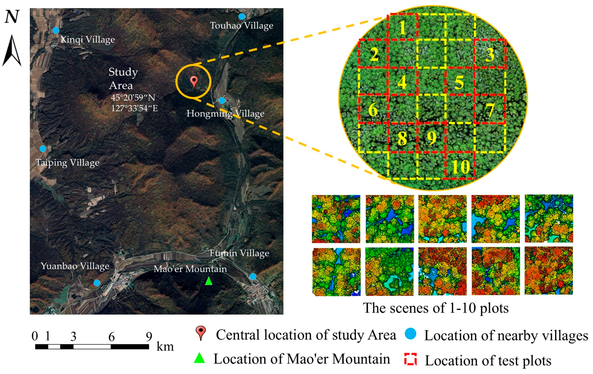

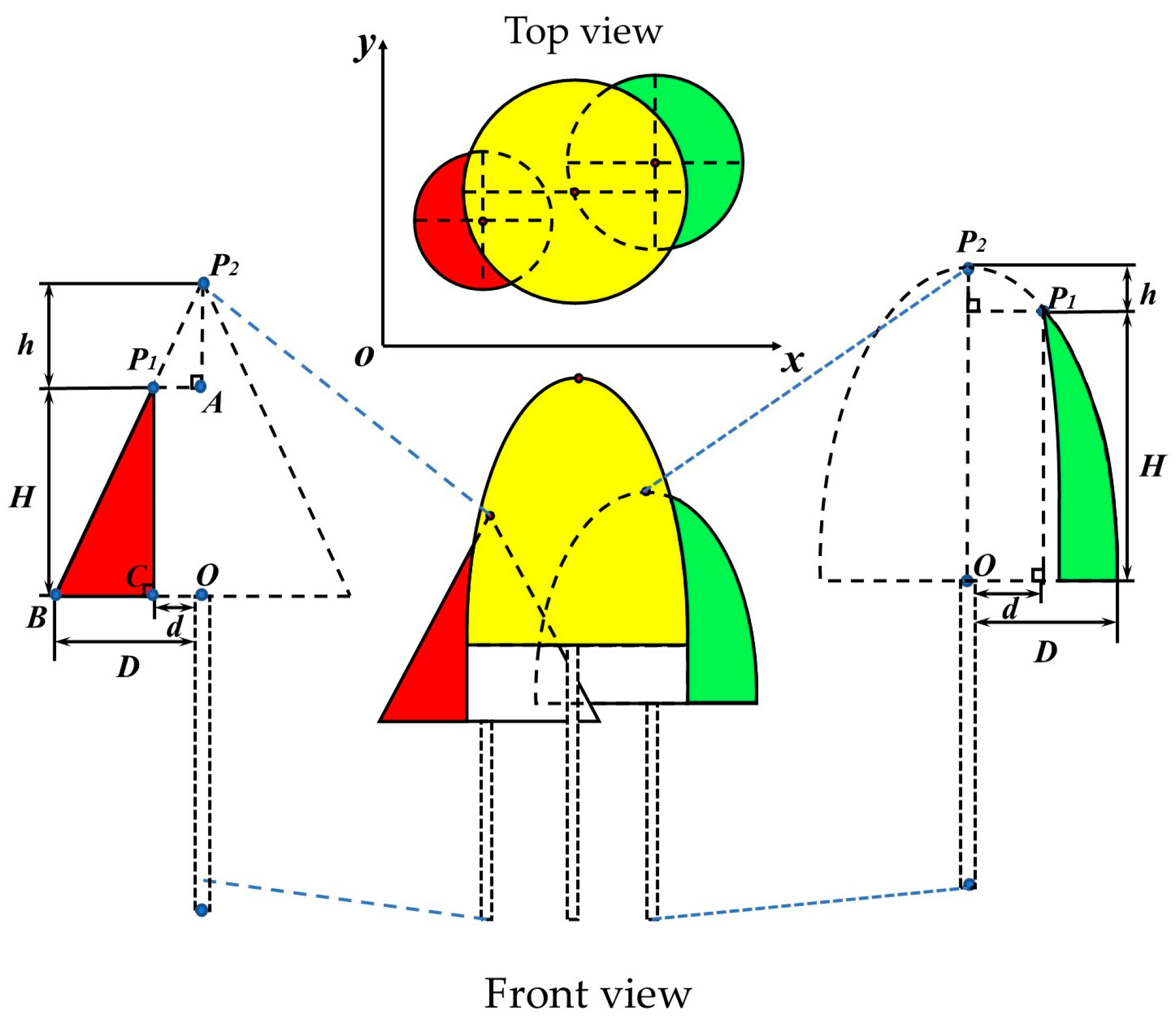
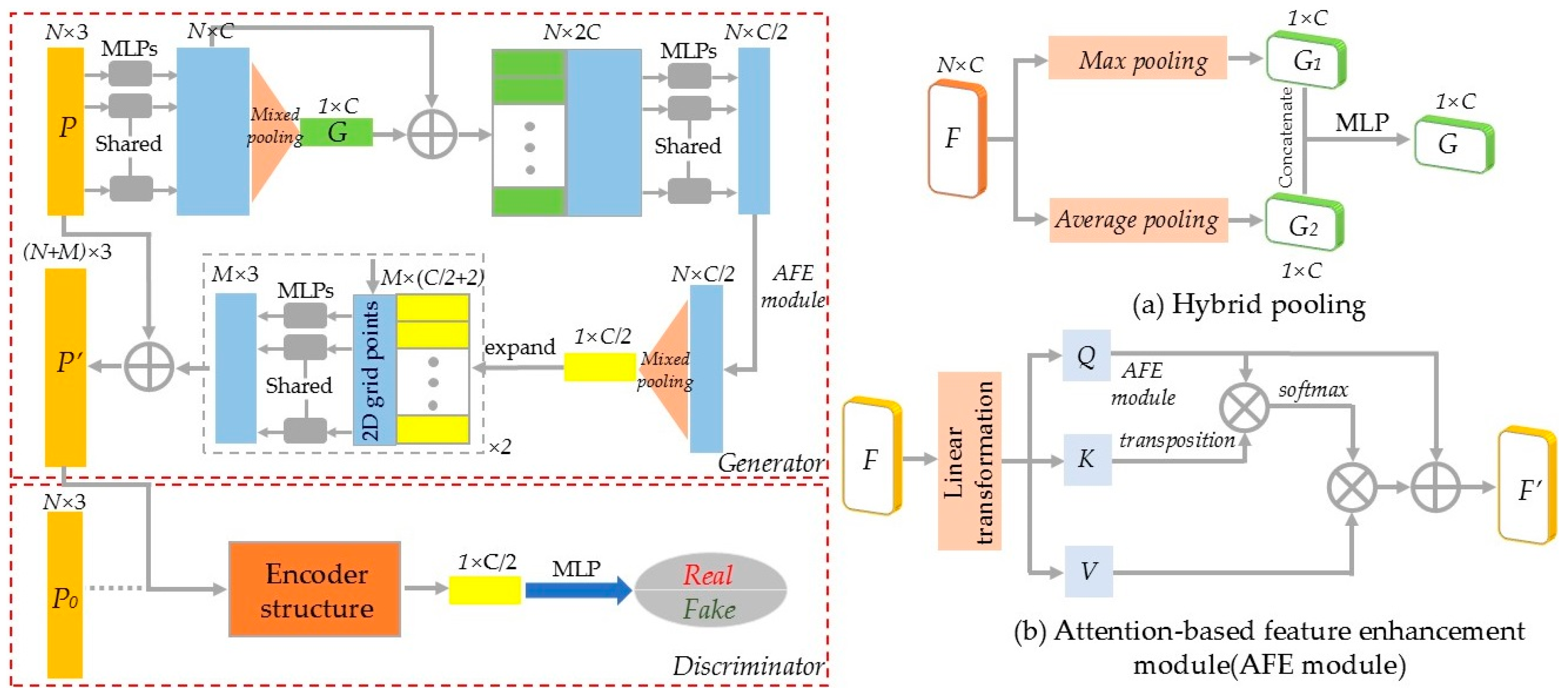
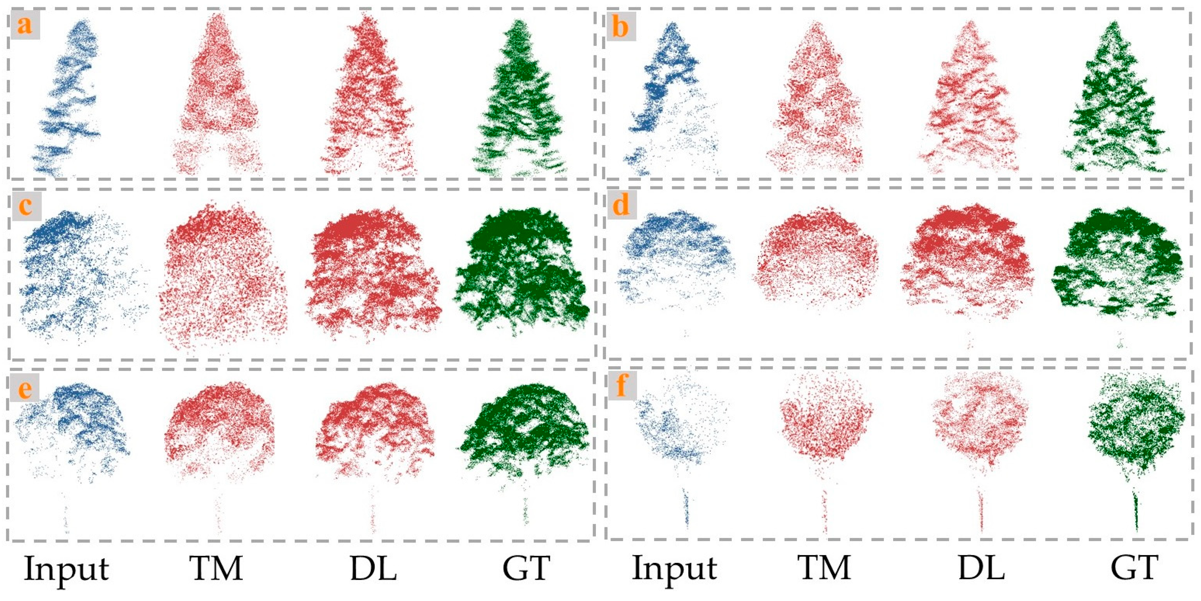
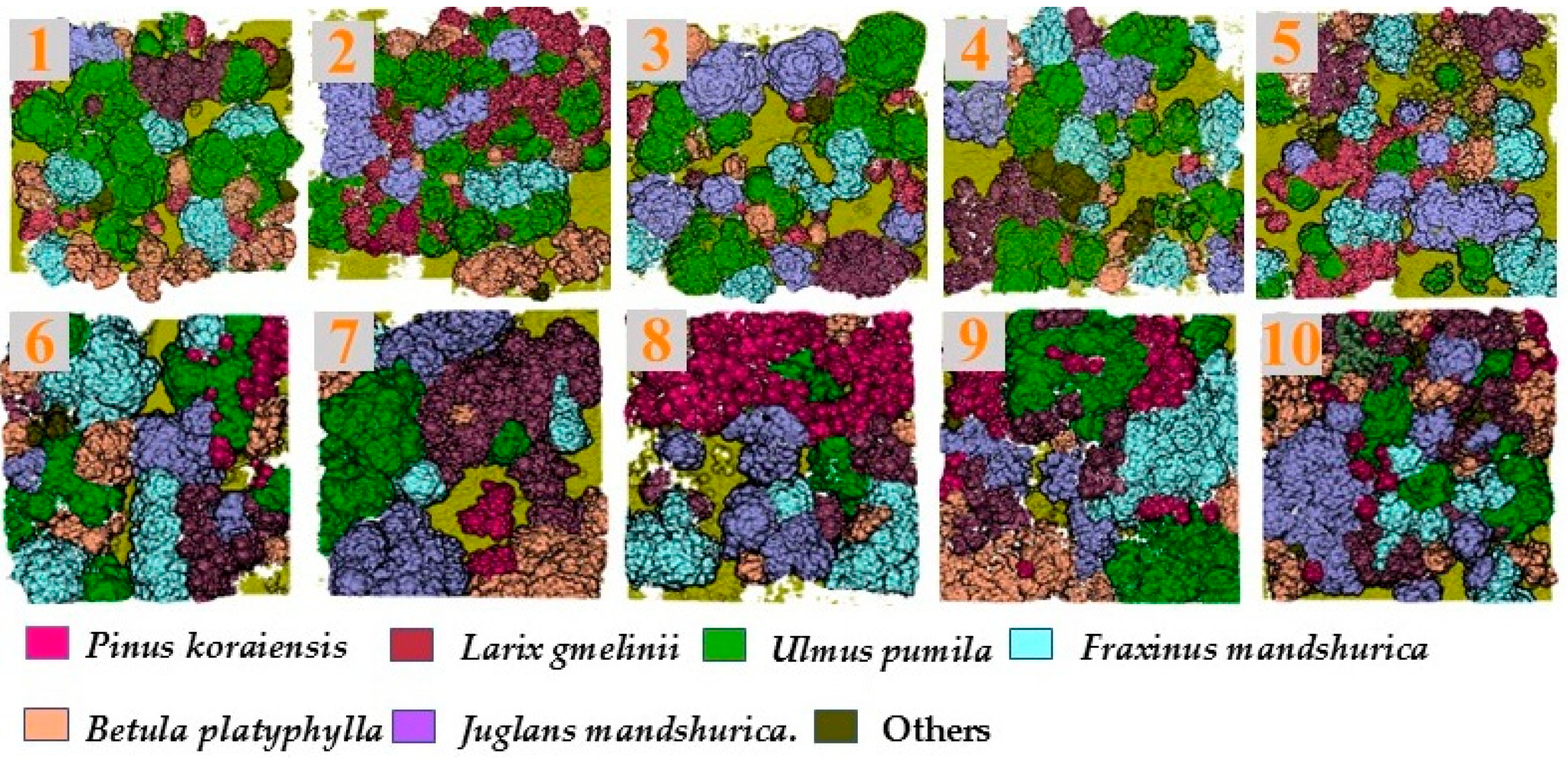
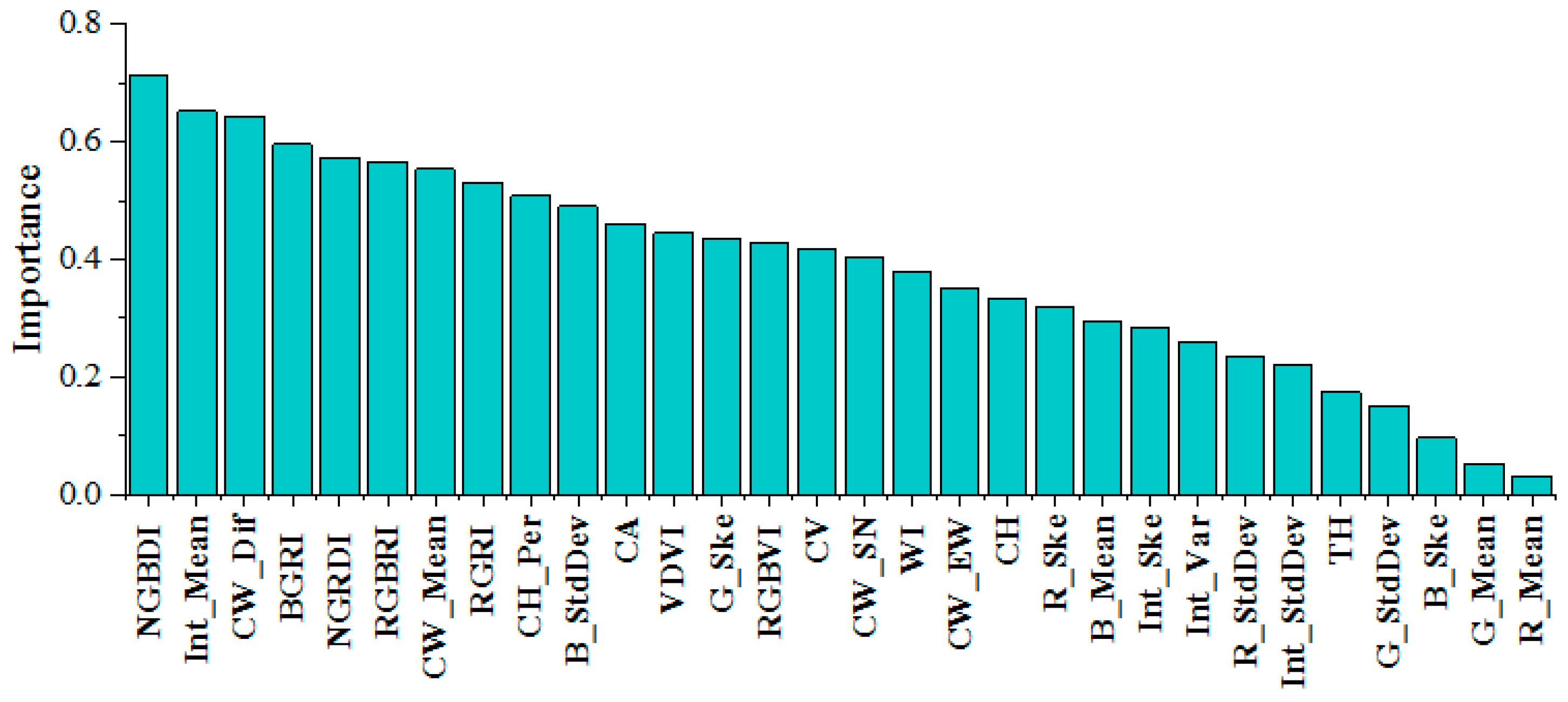
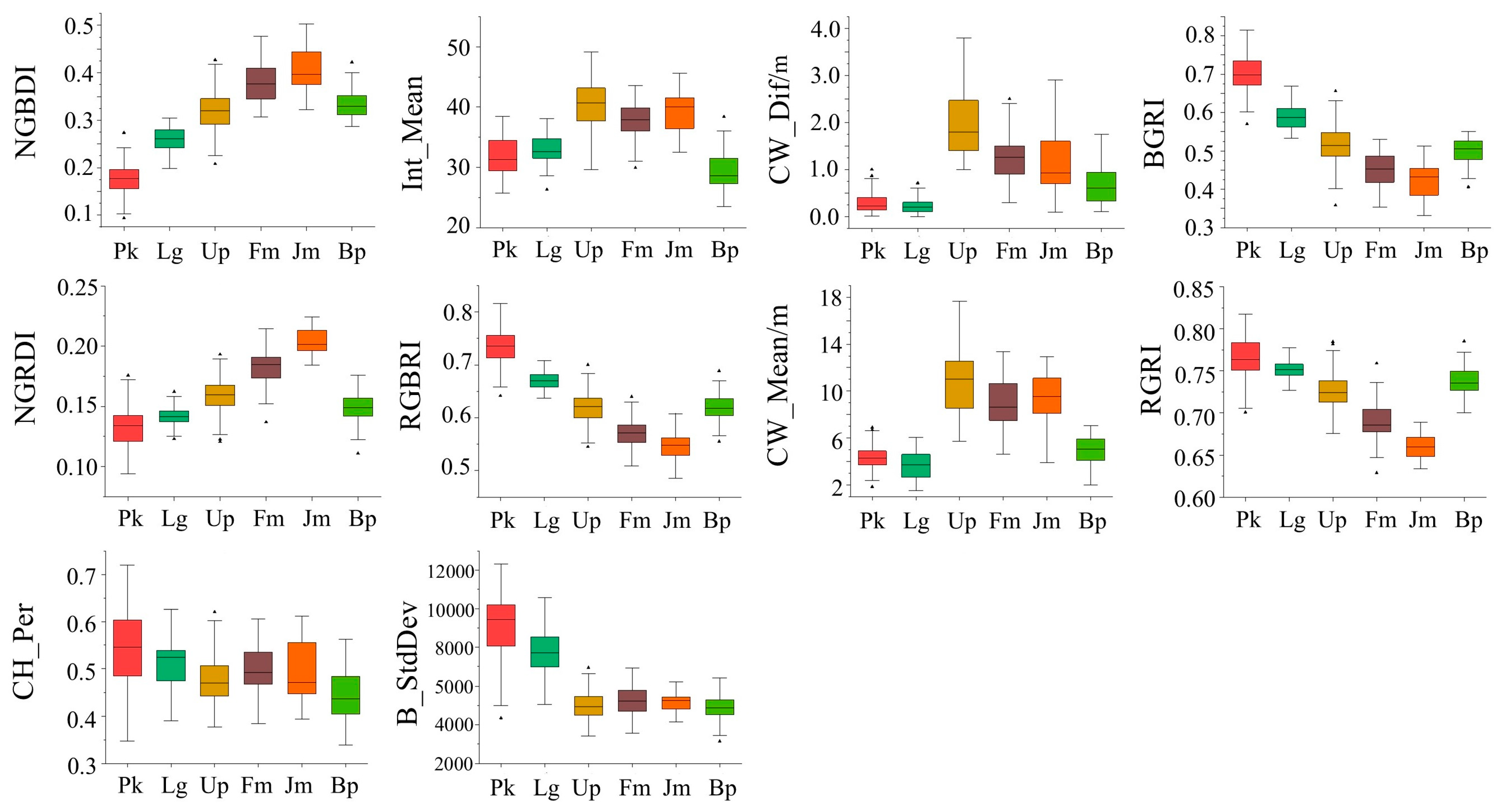
Disclaimer/Publisher’s Note: The statements, opinions and data contained in all publications are solely those of the individual author(s) and contributor(s) and not of MDPI and/or the editor(s). MDPI and/or the editor(s) disclaim responsibility for any injury to people or property resulting from any ideas, methods, instructions or products referred to in the content. |
© 2025 by the authors. Licensee MDPI, Basel, Switzerland. This article is an open access article distributed under the terms and conditions of the Creative Commons Attribution (CC BY) license (https://creativecommons.org/licenses/by/4.0/).