Article

Spatial Heterogeneity of Mountain Greenness and Greening in the Tibetan Plateau: From a Remote Sensing Perspective

1
School of Airport Economics and Management, Beijing Institute of Economics and Management, Beijing 100102, China
2
School of Information Engineering, China University of Geosciences, Beijing 100083, China
3
State Key Laboratory of Remote Sensing and Digital Earth, Faculty of Geographical Science, Beijing Normal University, Beijing 100875, China
*
Author to whom correspondence should be addressed.
Forests 2025, 16(4), 576; https://doi.org/10.3390/f16040576
Submission received: 10 February 2025 / Revised: 11 March 2025 / Accepted: 19 March 2025 / Published: 26 March 2025

Abstract

:
As an important component of terrestrial ecosystems, mountain vegetation serves as an indicator of climate change. Due to the sensitivity of the Tibetan Plateau Mountains (TPM) to climate change and their ecological fragility, their vegetation dynamics (greenness and greening) have become a hot spot issue in global environmental change. Topography is a relatively stable environmental factor that shapes vegetation by creating localized microenvironments. However, existing research primarily focuses on the effects of climate change and human activities on vegetation dynamics. Therefore, a more comprehensive understanding of the dependence of vegetation dynamics on topography is needed. To elucidate the relationship between topography and the spatial heterogeneity of vegetation dynamics, we conducted this study using the recently released high-precision Sensor-Independent Leaf Area Index product. Through long-term trend analyses and joint comparisons of multiple topographic variables, this study elucidates key patterns: (1) North-facing slopes exhibit higher vegetation greenness and stronger greening trends than south-facing slopes, whereas east- and west-facing slopes show comparable greenness but stronger greening on west-facing slopes. (2) Vegetation greenness and greening increase with slope steepness. (3) With increasing elevation, greenness decreases progressively, while greening follows a unimodal pattern—initially increasing, then decreasing, and nearing zero at high altitudes. These findings underscore the pivotal role of topography in regulating vegetation responses to climate change. This study provides new insights into the interplay between topography and vegetation dynamics, advancing our understanding of ecological processes on the TPM and informing strategies for ecosystem management under global warming.

1. Introduction

Vegetation participates in the exchange of carbon, water, momentum, and energy between the land and the atmosphere and is one of the main components of terrestrial ecosystems [1,2]. Mountains cover approximately 27% of the world’s land surface and mountain ecosystems provide many key ecosystem services [3,4,5]. As an important part of mountain ecosystems, mountain vegetation plays a crucial role in maintaining biodiversity, protecting water sources, conserving soil, storing carbon, and regulating the climate [6,7,8]. In addition, mountain vegetation is highly sensitive to global climate change and serves as an important indicator of climate change [5,9].
Vegetation greenness is a key indicator that characterizes aboveground green biomass, biochemical properties, and pigment composition [10,11]. A statistically significant increase in vegetation greenness at a specific location over a period of time is referred to as vegetation greening [12]. The greenness and greening directly affect the surface energy balance by influencing various biophysical factors, such as albedo and the proportion of solar radiation absorbed by the surface [13]. Vegetation greening may indicate an increase in land carbon sinks and can help mitigate the rise in global land surface temperatures [12,14]. Monitoring mountain vegetation dynamics is crucial for understanding changes in the structure and function of mountain ecosystems and their responses to various natural and anthropogenic driving factors. However, traditional ground-based observation methods are time-consuming and labor-intensive, making conducting large-scale and long-term monitoring of vegetation dynamics difficult. Remote sensing (RS) has become a key tool for monitoring vegetation dynamics over large areas due to its high efficiency, wide coverage, and diverse information [12,15,16]. Existing satellite observations indicate that since the early 1980s, global vegetation greenness has increased, and this is primarily attributed to higher carbon dioxide concentrations and their fertilization effect, global warming, and land use management [12,17,18,19].
The Tibetan Plateau (TP) is known as “the roof of the world” and “the third pole of the Earth”. Due to the climate sensitivity, biodiversity, and ecological fragility of the Tibetan Plateau Mountain (TPM), monitoring its vegetation dynamics is of great significance [20,21,22,23]. Most studies on the vegetation dynamics effects in the TP have primarily focused on analyzing its spatiotemporal patterns and the driving factors, such as climate [24,25,26]. Compared to climate change and human activities, topography (elevation, slope, and aspect) is a relatively constant environmental variable that can affect vegetation by creating a local microclimate [27,28,29,30]. Some existing studies use the Normalized Difference Vegetation Index (NDVI) as an indicator of greenness to analyze the relationship between vegetation and topographic factors. However, due to limitations such as soil background, atmospheric effects, saturation effects, and topographic effects, NDVI has certain limitations in monitoring vegetation dynamics [31,32,33,34].
In recent studies, the Leaf Area Index (LAI) has been widely used in the monitoring of vegetation dynamics due to its clear physical interpretation and close relationship with key ecological processes, such as photosynthesis, transpiration, and evaporation [12,35,36,37,38]. LAI is defined as half of the total green leaf area per unit of ground surface area and characterizes the structure of the vegetation canopy [39,40]. Stable and high-quality LAI products are crucial for ensuring the reliability of global and regional vegetation dynamics research [41]. Affected by adverse observation conditions such as large-angle observations and cloudy/rainy weather, many medium-resolution LAI remote sensing products suffer from issues such as incomplete spatiotemporal data and inconsistent internal accuracy [42,43]. The recently released Sensor-Independent LAI (SI LAI) product is based on high-quality retrievals from Terra-MODIS, Aqua-MODIS, and VIIRS standard LAI products, combined with a spatial–temporal tensor (ST-tensor) completion model [44]. Compared to the original MODIS products, the SI LAI product has achieved a comprehensive improvement in continuity and accuracy, providing more reliable data support for monitoring vegetation dynamics.
Elucidating the response mechanisms of vegetation greenness and greening to mountainous topography in the context of climate change is crucial for understanding the vegetation–climate response relationship and for addressing environmental challenges. The complex topography of the TPM makes it an ideal natural laboratory for studying the relationship between topography and vegetation dynamics. Therefore, this study is based on the SI LAI product from 2000 to 2022, combined with digital elevation model (DEM) data and trend analysis methods, to discuss the responses of vegetation greenness and greening in the TPM to topographic factors (elevation, slope, and aspect). Therefore, the objectives of this study were (a) to detect the spatial and temporal variations of vegetation greenness and greening in the TPM based on a long-term series dataset with high-quality LAI and (b) to find the relationship between spatial heterogeneity and topographic factors (elevation, slope, and aspect).

2. Materials and Methods

The specific technical workflow of this study is illustrated in Figure 1. First, remote sensing data were preprocessed by resampling the mountainous area identification data and DEM data to match the 500 m resolution of the SI LAI product. Then, vegetation greenness, greening, and topographic factors in the mountainous areas of the Tibetan Plateau were extracted. Finally, by constructing topographic grids, we quantified the dependence of vegetation greenness and greening on topographic factors.

2.1. Study Area

The TP is located in the southwest of China. It is the highest and largest plateau on Earth, with an average elevation exceeding 4000 m. It is renowned as “the Roof of the World” and “the Third Pole of the Earth” [45,46]. Due to its diverse topographic conditions and atmospheric circulation patterns, the TP exhibits remarkable climatic heterogeneity, characterized by a cold and arid alpine climate. The annual average temperature ranges from −3.1 °C to 4.4 °C, and the annual precipitation ranges from 103 mm to 694 mm, both decreasing from east to west [47,48,49,50]. The TP is home to vast mountainous areas, including the Kunlun Mountains, the Hengduan Mountains, the Tanggula Mountains, and the Himalayas. According to the MCD12Q1 data of 2022, grasslands dominate the vegetation in the TPM, covering 56% of the area (see Figure 2). Forests are mainly distributed in southern Tibet and southeastern TPM, accounting for 7.9%. Shrubs are mainly concentrated in the southeastern region, making up 3.6%. Croplands are incredibly scarce, accounting for less than 1%, and are distributed primarily in the Huangshui Valley in Qinghai. The elevation of the TPM generally exhibits a distribution pattern of higher altitudes in the west and lower altitudes in the east, with relatively steeper slopes in the southeastern areas. However, the distribution of slope aspects is highly heterogeneous.

2.2. Datasets

2.2.1. LAI Datasets

In this study, we used LAI to calculate the greenness and greening of vegetation in the TPM. The LAI dataset is from the Sensor-Independent LAI product (SI LAI product), which Boston University and Beijing Normal University collaboratively developed. This dataset builds a high-quality, sensor-independent LAI dataset based on the Terra-MODIS, Aqua-MODIS, and VIIRS LAI standard products using the spatial–temporal tensor (ST-tensor) completion model [44]. The dataset has a spatial resolution of 500 m, covers the period from 2000 to 2022, and has a temporal resolution of 8 days. Compared with similar datasets, the SI LAI product integrates high-quality observations from multiple satellite sensors and reconstructs the missing data, demonstrating remarkable spatiotemporal continuity and quality stability. These advantages ensure reliable long-term trend analysis, which is a crucial requirement for studying the vegetation dynamics in complex mountainous areas. It is available free of charge through the Google Earth Engine (https://code.earthengine.google.com/?asset=projects/sat-io/open-datasets/BU_LAI_FPAR/wgs_500m_8d, accessed on 21 March 2025).

2.2.2. Land Cover Data

The land cover data were obtained from the MODIS land cover type product (MCD12Q1 v061) (https://lpdaac.usgs.gov/products/mcd12q1v061/, accessed on 21 March 2025), which provides global land cover types at a spatial resolution of 500 m and annual intervals (2001 to present) [51]. The dataset contains five classification schemes, and for this study, the classifications under the International Geosphere-Biosphere Programme (IGBP) scheme were selected from 2001 to 2022. To focus more on the overall vegetation changes, we classified the biome types in the TPM into four major vegetation types: forests, shrubs, grasslands, and croplands. Evergreen needleleaf forests, evergreen broadleaf forests, deciduous needleleaf forests, mixed forests, and deciduous broadleaf forests were merged as forests. Closed shrublands, open shrublands, and woody savannas were merged as shrubs. Savannas, grasslands, and permanent wetlands were combined as grasslands. Croplands and cropland/natural vegetation mosaics were merged as croplands. In the analysis of vegetation types, only pixels where the vegetation type remained unchanged between 2001 and 2022 were used.

2.2.3. Mountain Range Identifier Data

The extent of the Tibetan Plateau’s mountains was determined using the high-resolution (7.5 arc second) binary raster file from the Global Mountain Biodiversity Assessment (GMBA Definition v2.0) (https://www.earthenv.org/mountains, accessed on 21 March 2025). The mountain definition in this data was directly derived from a DEM. A hierarchical structure was introduced to ensure global consistency and accuracy in the level of detail and resolution, and rivers were used to define the boundaries of contiguous mountain ranges [52]. To match the SI LAI product, the raster file was masked, nearest-neighbor resampled using ArcGIS 10.8, and its resolution was reduced to 500 m.

2.2.4. Digital Elevation Model Data

The elevation data are from the Advanced Spaceborne Thermal Emission and Reflection Radiometer (ASTER) Global Digital Elevation Model Version 3 (GDEM V3), which has a spatial resolution of approximately 30 m (https://lpdaac.usgs.gov/products/astgtmv003/, accessed on 21 March 2025). The GDEM V3 was released in 2019, using new custom software to eliminate most artifacts and adding 200,000 scenes to fill the holes [46]. We used GDEM V3 to compute elevation, slope, and aspect data of the Tibetan Plateau Mountains and then used a bilinear method to resample these topographic factors to 500 m to match the SI LAI product.

2.3. Methods

2.3.1. Extraction of Greenness and Greening

In this study, we used the growing season-averaged LAI to describe vegetation greenness in the TPM. Based on previous studies, the growing season was defined as May to September each year [53,54]. The time-series trend of vegetation greenness from 2000 to 2022 was used to characterize vegetation greening. The trend was calculated using the Theil-Sen trend analysis method, which is a non-parametric estimator and can effectively eliminate the influences of outliers in long-term series trend analysis compared to ordinary least squares linear regression [55,56]. The g r e e n i n g is calculated as follows:
G r e e n i n g = m e d i a n x j x i j i , ( 2000 i j 2022 )
where x j and x i represent the vegetation greenness in the j and i year, respectively. If G r e e n i n g > 0, it is indicated as an increasing trend of greenness, conversely decreasing trend.
The Mann–Kendall (MK) test was used to determine the significance of greening. The MK test is a nonparametric statistical method that does not require the sample to follow any particular distribution and reduces the effect of outliers [57,58,59]. The MK test is calculated as follows:
S = i = 1 n 1 j = i + 1 n s g n x j x i
where x i and x j represent the value of a pixel of i and j year, respectively, and satisfy (3):
s g n x j x i = + 1       x j x i > 0   0           x j x i = 0 1       x j x i < 0
The variance estimate for S is calculated as follows:
v a r S t = n n 1 2 n + 5 p = 1 m t p ( t p 1 ) ( 2 t p + 5 ) 18
where m represents the number of tied groups, and t p represents the amount of data in the p-th the group. The standardized MK statistic Z is calculated as follows:
Z = S t 1 v a r ( S t )               S t > 0             0                           S t = 0 S t + 1 v a r ( S t )               S t < 0
The null hypothesis is rejected when |Z| > Z1–α/2, where α is the statistical significance level concerned. When |Z| is greater than or equal to 1.64 (α = 0.1), 1.96 (α = 0.05), and 2.58 (α = 0.01), the time series passes the significance test at 90%, 95%, and 99% confidence levels, respectively. Based on previous studies [19], we consider greening to be statistically significant when |Z| is greater than or equal to 1.64 (p < 0.1).

2.3.2. Dependence Analysis on Topographic Factors

To investigate the dependence of vegetation greenness and greening on topographic factors, we divided the pixels into two groups of four types based on aspect: south-facing slopes (SFSs) and north-facing slopes (NFSs), as well as east-facing slopes (EFSs) and west-facing slopes (WFSs). The SFS was defined as pixels with aspect values between 135 and 225°, NFS as pixels with aspect values between 315 and 360° or 0 and 45°, EFS as pixels with aspect values between 45 and 135°, and WFS as pixels with aspect values between 225 and 315°. Then, the mean values of greenness and greening were calculated separately for each 10 × 10 km grid (20 × 20 pixels) for each facing slope. We also calculated the mean elevation and mean slope of the grids, and grids with contrasting aspects that differed in elevation by more than 500 m and in slope by more than 5° were masked out to minimize the effect of elevation and slope differences on the aspect analysis. Additionally, we set the grids with fewer than 10 valid pixels to null to ensure the relative robustness of the analysis results. In order to quantify the symmetry of greenness and greening on contrasting aspects, we propose the greenness symmetric index (GreSI) and the greening symmetric index (GrnSI). GreSI and GrnSI are calculated as follows:
G r e S I = G r e e n n e s s i G r e e n n e s s j
G r n S I = G r e e n i n g i G r e e n i n g j
where i and j represent a pair of contrasting aspects (SFS vs. NFS, EFS vs. WFS), and G r e e n n e s s i , j and G r e e n i n g i , j represent the average values of greenness and greening (p < 0.1) in the grid. The closer the GreSI is to 1, the more symmetrical the greenness of contrasting aspects becomes. If GreSI > 1, it indicates that the SFS (EFS) is greener than the NFS (WFS). The closer the GrnSI is to 0, the more symmetrical the greening of contrasting aspects becomes. If GrnSI > 0, it indicates that the greening intensity of the SFS (EFS) is stronger than that of the NFS (WFS).
In addition, we constructed a topographic grid with an elevation interval of 125 m and a slope interval of 1° and further investigated the dependence of vegetation greenness and greening on elevation and slope by calculating the average greenness and greening of each grid. To avoid the effect of extreme values, we set the grids with less than 20 effective pixels as null values.

3. Results

3.1. Spatial Patterns of Greenness

Vegetation greenness in the TPM shows a spatial distribution pattern of high in the southeast and low in the northwest (Figure 3a), which conforms to the distribution pattern of the hydrothermal gradient in the TPM. The region with the highest greenness is in the southern TPM, where the vegetation type is dominated by forests with greenness ranging from 4 to 6. The region with the lowest greenness is in the southwestern TPM, where grasslands dominate the vegetation type, and the greenness ranges between 0 and 1. The average greenness of the entire TPM is 1.19, and the frequency histogram curve (green line) and cumulative frequency curve (red line) show that the majority of the TPM area has relatively low greenness, with over 90% of the greenness being less than 3 (Figure 3b). Figure 3c shows the boxplot of the different land cover types’ greenness, which shows that forest vegetation exhibits the highest greenness, followed by shrubs, then cropland, and grassland having the lowest greenness.
From 2000 to 2022, the interannual variation in average greenness increased significantly (p < 0.01) for all vegetation types (Figure 4). Among them, the cropland exhibited the most rapid increase, at approximately 0.0119/yr, while the grassland demonstrated a relatively slower rate of increase, at 0.0038/yr.

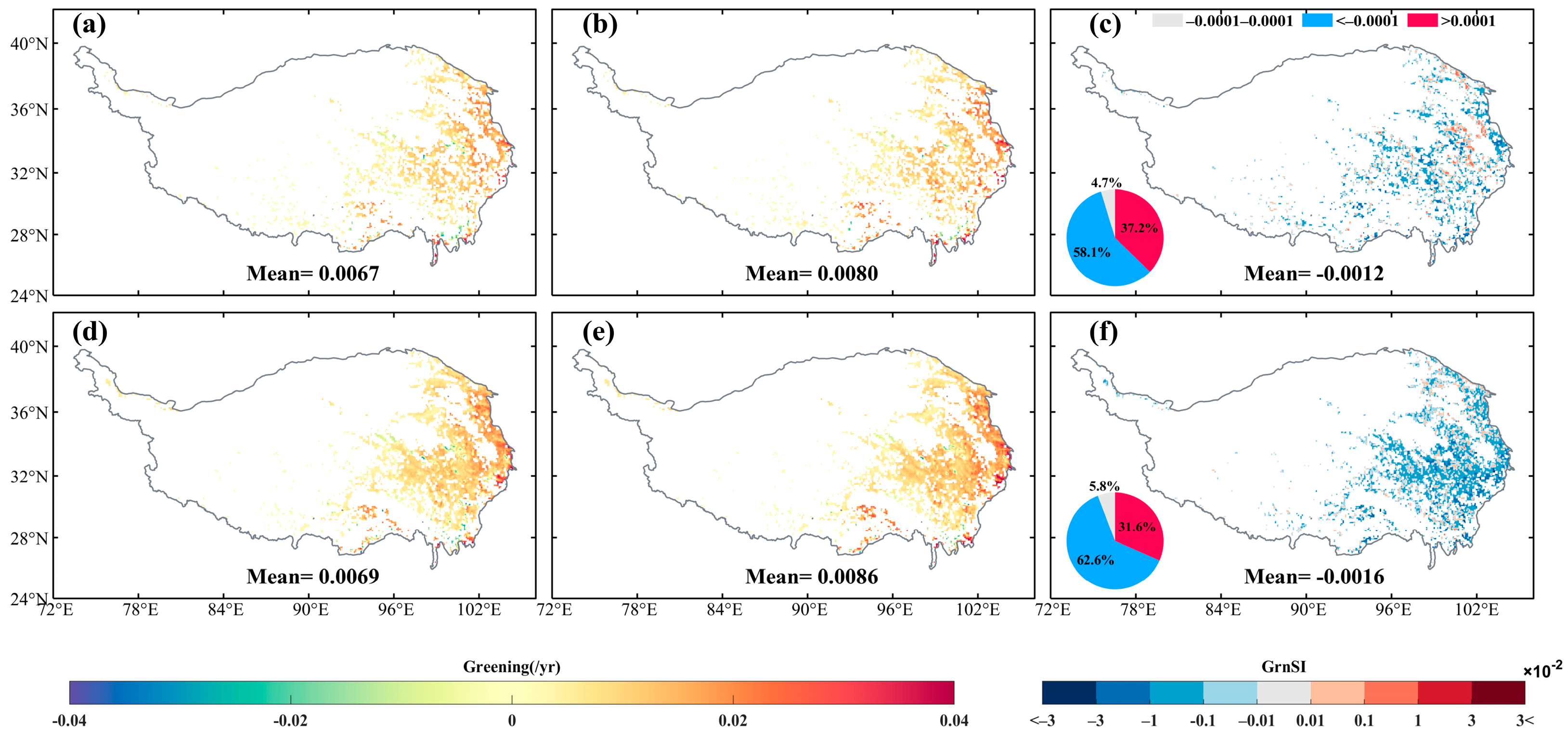
3.2. Spatial Patterns of Greening

The vegetation greening in the TPM shows a decreasing trend from northeast to southwest, ranging from −0.03 to 0.03 (Figure 5a). The greening of southwest TPM vegetation was very close to 0, while the northeastern TPM vegetation had the highest greening with close to 0.03/yr. Furthermore, the areas with no significant changes were mainly concentrated in the southwestern TPM (Figure 5b), where the main vegetation type was grasslands. Vegetated areas in the northeastern TPM predominantly show a significant increase in greening, while the distribution of pixels with a significant decrease in vegetation is more random. As shown in Figure 5c, 37.1% of vegetated areas in the TPM show a significant increase, 4.7% show a significant decrease (p < 0.1), and the remaining 58.1% exhibit no significant changes. Moreover, among the vegetation pixels that passed the MK test (p < 0.1), 88.66% are greening and 11.33% are browning, with a mean greening rate of 0.01/yr (see Figure 5b).
Based on the greening and MK test, we divided the greening trend of various vegetation types into three types (Figure 5d). From the vegetation types, croplands had the highest percentage of pixels with a significant increase in greening as a percentage of its total pixel count, close to 60%, while the other vegetation types ranged from 20% to 40%, and 3%–10% of pixels per vegetation type showed significant decreases. The frequency distribution plot shows that the greening of the various vegetation types was concentrated in the range of −0.05 to 0.05/yr (Figure 6). Croplands and forests had the highest levels of greening, with average greening values of 0.018/yr and 0.017/yr, respectively. In contrast, grasslands and shrubs showed lower average greening of 0.007/yr and 0.014/yr, respectively. Additionally, the grasslands had a unimodal distribution and a peaked location closer to 0. However, other types exhibited a bimodal distribution. These results indicate that the greenness of the grasslands is more stable.

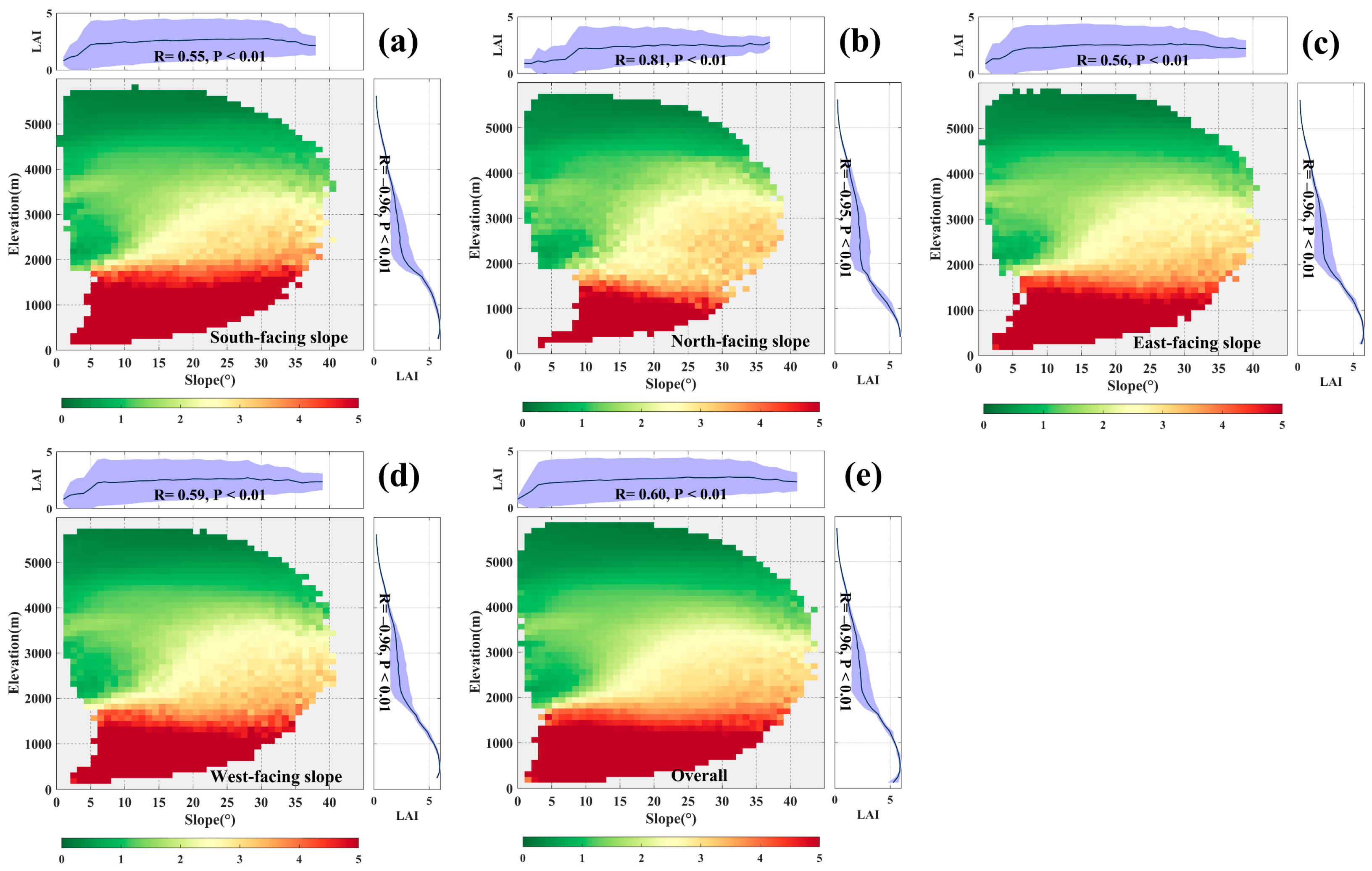
3.3. Dependence of Vegetation Greenness on Topography

Figure 7 illustrates the spatial distribution of vegetation greenness and GreSI across different aspects in the TPM. Overall, the vegetation greenness is higher on the NFS compared to the SFS, with a mean greenness of 1.0673 for the SFS and 1.111 for the NFS. The GreSI distribution between the SFS and NFS (Figure 7c) indicates that the NFS generally has superior vegetation greenness, with an average GreSI value of 0.959. The pie chart further quantifies this difference, indicating that in 61.9% of the area, the SFS has lower greenness than the NFS, while 5.7% displays similar greenness on both slopes (GreSI between 0.99 and 1.01). Approximately 32.4% of the area, primarily in southern Tibet, exhibits higher greenness on the SFS compared to the NFS. The mean greenness of the EFS and WFS is approximately 1.08, indicating minimal overall differences in vegetation greenness. The mean value of the GreSI between the EFS and WFS is 1.0065 (Figure 7f), suggesting near-symmetry in vegetation greenness between the east- and west-facing slopes. In 47.6% of the area, the EFS has lower greenness than the WFS, while in 43.9%, the EFS exhibits higher greenness than the WFS.
We analyzed the variation in greenness across different aspects of elevation and slope space (Figure 8). Vegetation greenness in the TPM shows a significant dependence on elevation and slope, as evidenced by the fact that greenness increases with increasing slope and decreases with increasing elevation but is more dependent on elevation. The correlation coefficient R between greenness and elevation ranges between −0.95 and −0.96 among the five aspect classification schemes (p < 0.01), indicating a very strong, significant negative correlation. The correlation between greenness and slope is relatively low, ranging from 0.55 to 0.60 (p < 0.01), except for the NFS, where R equals 0.81. From the perspective of the standard deviation of greenness (indicated by the blue shadow), the standard deviation at the same slope but different elevations is greater compared to the standard deviation at the same elevation but different slopes. This indicates that the variability in vegetation greenness caused by changes in elevation is stronger. In addition, it is worth noting that the greenness of the vegetation varies most markedly with the slope in the range of 2000 m to 3500 m.

3.4. Dependence of Vegetation Greening on Topography

Figure 9 shows the spatial distribution of greening intensity for different slope orientations as well as the degree of symmetry on contrasting aspects. The average greening of the south-, north-, east-, and west-facing slopes differs. The vegetation greening is stronger on the NFS than on the SFS and on the WFS than on the EFS. The mean greening is 0.0067/yr for the SFS and slightly higher at 0.0080/yr for the NFS. For both east- and west-facing slopes, the WFS had the highest mean greening at 0.0086/yr, and the EFS had an average greening of 0.0069/yr. The GrnSI further emphasizes the influence of slope orientation on vegetation greening. About 58.1% of the north–south-facing slopes exhibit a GrnSI less than −0.0001/year, with an average GrnSI of −0.0012/year, suggesting that the SFS is generally weaker than the NFS in terms of greening intensity in the TMP. About 62.6% of the east–west-facing slopes show a GrnSI less than −0.0001/year, with an average GrnSI of −0.0016/year. The greening asymmetry of east–west-facing slopes is slightly higher than that of north–south-facing slopes.
The distribution of vegetation greening across different slope aspects in elevation and slope space is shown in Figure 10. In the topographic space, we found a strong dependence of greening on elevation and slope. In the classifying of five slope orientations, the areas with the highest vegetation greening are found at elevations between 1000 and 3000 m and slopes ranging from 15° to 35°. In contrast, vegetation below 1000 m shows overall browning. Through analyzing the variation of greening with elevation and slope, we found that greening significantly increases with slope, while the intensity of greening first strengthens and then weakens with rising elevation, eventually approaching 0. Among all slope orientations, the WFS showed the highest positive correlation between greening and slope (R = 0.97, p < 0.01), while the EFS had the lowest correlation (R = 0.48, p < 0.01). When slope orientation was not distinguished, the correlation between greening and slope remained high (R = 0.95, p < 0.01). Additionally, the change in greening with elevation appeared to be nonlinear; as elevation increased, greenness shifted from negative to positive, reaching a peak around 2000 m before declining, approaching 0 above 5000 m. However, due to the limited effective grid points for the NFS below 2000 m, greening on the NFS continuously decreased starting from 2000, showing a significant negative correlation (R = −0.98, p < 0.01), which indirectly illustrates the strong nonlinear relationship between greening and elevation.

4. Discussion

4.1. Spatial Heterogeneity of Vegetation Greenness and Greening

The vegetation greenness and greening in the TPM exhibit noticeable spatial heterogeneity. Results indicate that the greenness in these areas shows a southeast-high and northwest-low distribution pattern. Vertically, vegetation greenness gradually decreases with increasing altitude. In terms of slope aspect distribution, the greenness on the NFS is generally higher than on the SFS, while the greenness on the EFS is similar to that on the WFS. Additionally, at the same altitude, areas with gentler slopes tend to have lower greenness, whereas areas with steeper slopes tend to have higher greenness.
The vegetation greening in the TPM exhibits an east-high and west-low spatial distribution pattern. Over one-third of the mountainous vegetation shows significant greening (p < 0.1). Vertically, greening first increases and then decreases with altitude, approaching zero at high altitudes. In terms of slope aspect distribution, the greening on the NFS is usually stronger than on the SFS, while the greening on the WFS is stronger than on the EFS. Furthermore, at the same altitude, areas with gentler slopes tend to have slightly weaker greening compared to areas with steeper slopes.

4.2. Dominant Factors Contributing to the Spatial Heterogeneity of Vegetation Greenness and Greening

The spatial heterogeneity of topographic factors (elevation, slope, and aspect) in mountain ecosystems leads to heterogeneity in factors such as solar radiation intensity, precipitation, temperature, evapotranspiration, carbon dioxide concentration, soil conditions, human activity intensity, and monsoon systems (Figure 11). This creates local or regional microenvironments with different hydrothermal conditions, which in turn leads to real heterogeneity in vegetation greenness and greening [27,28,60].
Hydrothermal conditions are the main nonbiological factors determining vegetation greenness [61,62]. The topographic heterogeneity of the TP creates pronounced microclimate differences, leading to variations in hydrothermal conditions that determine vegetation growth. From a vertical perspective, both surface air temperature and rainy season precipitation in the TP region decrease with increasing elevation [63,64]. This creates a vertical vegetation belt from forest to grassland to sparse vegetation [54,65], leading to vertical heterogeneity in vegetation greenness. In addition, different aspects exhibit variations in light intensity, humidity, temperature, and soil conditions [66]. SFSs are relatively warm and dry in temperature-limited areas, resulting in higher vegetation greenness. In contrast, NFSs have higher vegetation greenness in precipitation-limited areas due to their cold and moist conditions [28]. Slope can influence vegetation greenness by shaping soil moisture, soil erosion rates, and litter accumulation [60]. In the vegetation of the TP, forests and shrubs grow in areas with the steepest slopes, while grasslands are concentrated in flatter areas [67,68]. Therefore, the observed differences in vegetation greenness across different slopes are mainly due to the different vegetation types in those areas.
Vegetation greening on the TP is thought to be primarily driven by climate change, especially warming and wetting [69,70]. The heterogeneity of topographic factors leads to differences in vegetation response patterns to climate change. In low-altitude areas with suitable temperatures, vegetation greenness is more sensitive to precipitation, while in cooler high-altitude areas, a slight increase in temperature may enable vegetation to achieve a better water-thermal balance [71,72,73]. In the low-altitude regions of the TP, precipitation shows a decreasing trend [74,75], and warming will exacerbate drought conditions, suppressing vegetation growth and leading to vegetation browning. In the mid-altitude regions, the warming and humidification of the climate bring vegetation closer to the optimal water-thermal balance needed for growth, resulting in the strongest greening trend. Although both precipitation and temperature affect vegetation greenness, existing studies indicate that temperature contributes more to greening on the TP [76]. Therefore, from the perspective of the NFS, which provides greater moisture, they can better benefit from climate warming concerning vegetation greening. Research on the greening differences between the EFS and WFS is limited. The greening trend is stronger on the WFS than on the EFS, possibly because the WFSs are more influenced by the Indian monsoon, while the EFSs are more affected by the East Asian monsoon. Existing studies have shown that the increase in rainfall from the Indian summer monsoon on the TP far exceeds that from the East Asian summer monsoon [77]. The Indian monsoon has been continuously strengthening since 2002 [78]. In addition, the weakening of westerly wind may lead to increased humidity in the arid and semi-arid regions of the TP, potentially benefiting the WFS more, which results in the asymmetry in greening between the WFS and EFS [79]. Another possible factor is that the WFS receives solar radiation on warm afternoons and interacts with increased precipitation to promote vegetation greening. Regarding slope, steep slopes primarily support the growth of forests and shrubs, which show a stronger greening trend (Figure 5). This may be because these two vegetation types benefit more from climate change. In addition, variations in wind patterns, monsoon intensity, precipitation mechanisms, evapotranspiration processes, soil types, groundwater levels, and snow and ice coverage caused by topography also contribute to the spatiotemporal heterogeneity of ecosystem processes and surface characteristics.
Finally, topography is closely related to human activities. The higher population and livestock density in low-altitude areas may negatively impact vegetation [54]. In addition, since 2000, China has implemented the “returning farmland to forest” strategy, aiming to convert cultivated land with slopes exceeding 25° into forested areas. This strategy has promoted greening on the steep slopes of the TPM [80,81].

4.3. Uncertainty and Limitations of the Study

The observed spatial heterogeneity of vegetation greenness and greening includes not only real heterogeneity but also artificial heterogeneity arising from remote sensing observations (Figure 10). These artificial heterogeneities arise from atmospheric effects, observation conditions, topographic effects, sensor issues, and BRDF effects, among others [32,71,72,73]. In this study, we employed the SI LAI product to infer vegetation dynamics, which significantly alleviates common challenges such as adverse observation conditions and inconsistencies in internal algorithms. However, the SI LAI product may still exhibit certain limitations. Uncertainties persist due to variations in observation conditions, the influence of BRDF effects, and inherent constraints of remote sensing data. Furthermore, since the SI LAI product is derived from the MODIS LAI product, it may inherit some of the limitations of the latter. For instance, the retrieval algorithms for MODIS LAI and most medium-spatial-resolution LAI products are better suited for horizontal surfaces but inadequately account for topographic effects [74]. This insufficient consideration of terrain may have a detrimental impact on vegetation monitoring in mountainous areas, particularly when the topography is highly rugged [75].
In addition, the growing season of vegetation on the TP exhibits spatial heterogeneity, and due to rising temperatures and increased precipitation, the start of the growing season advanced by 8.3 ± 2.0 days, while the end of the season was delayed by 8.2 ± 1.9 days during the period from 2000 to 2020 [82]. These changes may not have been fully reflected during the study period. Finally, there are differences in the physiological characteristics of different vegetation types. In future studies, it is essential to conduct in-depth research on the relationship between the greenness and greening of different vegetation types and topography.

5. Conclusions

In the global climate change context, topography is a relatively constant environmental factor influencing vegetation dynamics. Understanding the response mechanism of vegetation dynamics to topography in the TPM can enhance our comprehension of the vegetation–climate response relationship. In this study, we analyzed the relationships between vegetation greenness and greening and factors such as elevation, slope, and aspect from 2000 to 2022 in the TPM. The results indicate that approximately 37.1% of the vegetation in the TPM region is significantly greening, and the spatial distribution of greenness and greening exhibits spatial heterogeneity. Specifically, greenness shows a pattern of being higher in the southeast and lower in the northwest, while greening is stronger in the northeast and weaker in the southwest. Furthermore, this spatial heterogeneity is closely related to topographic factors. We found that both greenness and greening on the NFS are higher than those on the SFS, while greening on the WFS is stronger than that on the EFS. Both greenness and greening increase with slope. As elevation increases, greenness continuously decreases, while greening initially strengthens and then weakens, ultimately approaching 0. Overall, topographic conditions can regulate local areas’ moisture and thermal conditions, creating microclimates that determine whether vegetation can benefit from climate change. Research on the regulatory effects of topography on vegetation greenness and greening is relatively scarce. Our study provides valuable insights into the vegetation dynamics of the TPM and offers a scientific basis for the restoration and management of mountainous vegetation in the context of global climate change [83].

Author Contributions

Conceptualization, Z.L. and J.L.; methodology, Z.L.; software, X.Z.; validation, S.Z.; formal analysis, X.Z.; investigation, X.Z. and S.Z; resources, J.L.; data curation, X.Z.; writing—original draft preparation, Z.L. and X.Z.; writing—review and editing, J.L, S.Z. and P.L.; visualization, X.Z. and S.Z.; supervision, J.L.; project administration, J.L.; funding acquisition, J.L. All authors have read and agreed to the published version of the manuscript.

Funding

This research was funded by the National Natural Science Foundation of China, grant numbers 42401439 and 42271356, and the Fundamental Research Funds for the Central Universities.

Data Availability Statement

The raw data supporting the conclusions of this article will be made available by the authors upon request.

Conflicts of Interest

The authors declare no conflicts of interest.

References

  1. Bonan, G.B.; Pollard, D.; Thompson, S.L. Effects of boreal forest vegetation on global climate. Nature 1992, 359, 716–718. [Google Scholar] [CrossRef]
  2. Zhong, L.; Ma, Y.; Salama, M.S.; Su, Z. Assessment of vegetation dynamics and their response to variations in precipitation and temperature in the Tibetan Plateau. Clim. Change 2010, 103, 519–535. [Google Scholar] [CrossRef]
  3. Messerli, B.; Ives, J.D. Mountains of the World: A Global Priority; Parthenon Publishing Group: Carnforth, UK, 1997. [Google Scholar]
  4. Schröter, D.; Cramer, W.; Leemans, R.; Prentice, I.C.; Araújo, M.B.; Arnell, N.W.; Bondeau, A.; Bugmann, H.; Carter, T.R.; Gracia, C.A. Ecosystem service supply and vulnerability to global change in Europe. Science 2005, 310, 1333–1337. [Google Scholar] [CrossRef] [PubMed]
  5. Kumar, P. The Economics of Ecosystems and Biodiversity: Ecological and Economic Foundations; Routledge: London, UK, 2012. [Google Scholar]
  6. Ma, S.; Qiao, Y.-P.; Wang, L.-J.; Zhang, J.-C. Terrain gradient variations in ecosystem services of different vegetation types in mountainous regions: Vegetation resource conservation and sustainable development. For. Ecol. Manag. 2021, 482, 118856. [Google Scholar] [CrossRef]
  7. Strand, J.; Soares-Filho, B.; Costa, M.H.; Oliveira, U.; Ribeiro, S.C.; Pires, G.F.; Oliveira, A.; Rajão, R.; May, P.; Van Der Hoff, R. Spatially explicit valuation of the Brazilian Amazon forest’s ecosystem services. Nat. Sustain. 2018, 1, 657–664. [Google Scholar]
  8. Onaindia, M.; de Manuel, B.F.; Madariaga, I.; Rodríguez-Loinaz, G. Co-benefits and trade-offs between biodiversity, carbon storage and water flow regulation. For. Ecol. Manag. 2013, 289, 1–9. [Google Scholar]
  9. Rogora, M.; Frate, L.; Carranza, M.L.; Freppaz, M.; Stanisci, A.; Bertani, I.; Bottarin, R.; Brambilla, A.; Canullo, R.; Carbognani, M. Assessment of climate change effects on mountain ecosystems through a cross-site analysis in the Alps and Apennines. Sci. Total Environ. 2018, 624, 1429–1442. [Google Scholar]
  10. Huang, H.; Xi, G.; Ji, F.; Liu, Y.; Wang, H.; Xie, Y. Spatial and temporal variation in vegetation cover and its response to topography in the selinco region of the qinghai-tibet plateau. Remote Sens. 2023, 15, 4101. [Google Scholar] [CrossRef]
  11. An, S.; Zhu, X.; Shen, M.; Wang, Y.; Cao, R.; Chen, X.; Yang, W.; Chen, J.; Tang, Y. Mismatch in elevational shifts between satellite observed vegetation greenness and temperature isolines during 2000–2016 on the Tibetan Plateau. Glob. Change Biol. 2018, 24, 5411–5425. [Google Scholar]
  12. Piao, S.; Wang, X.; Park, T.; Chen, C.; Lian, X.; He, Y.; Bjerke, J.W.; Chen, A.; Ciais, P.; Tømmervik, H. Characteristics, drivers and feedbacks of global greening. Nat. Rev. Earth Environ. 2020, 1, 14–27. [Google Scholar]
  13. Chen, C.; Li, D.; Li, Y.; Piao, S.; Wang, X.; Huang, M.; Gentine, P.; Nemani, R.R.; Myneni, R.B. Biophysical impacts of Earth greening largely controlled by aerodynamic resistance. Sci. Adv. 2020, 6, eabb1981. [Google Scholar] [PubMed]
  14. Feng, H.; Zou, B. A greening world enhances the surface-air temperature difference. Sci. Total Environ. 2019, 658, 385–394. [Google Scholar] [PubMed]
  15. Camps-Valls, G.; Campos-Taberner, M.; Moreno-Martínez, Á.; Walther, S.; Duveiller, G.; Cescatti, A.; Mahecha, M.D.; Muñoz-Marí, J.; García-Haro, F.J.; Guanter, L. A unified vegetation index for quantifying the terrestrial biosphere. Sci. Adv. 2021, 7, eabc7447. [Google Scholar] [PubMed]
  16. Gao, S.; Yan, K.; Liu, J.; Pu, J.; Zou, D.; Qi, J.; Mu, X.; Yan, G. Assessment of remote-sensed vegetation indices for estimating forest chlorophyll concentration. Ecol. Indic. 2024, 162, 112001. [Google Scholar]
  17. Pan, N.; Feng, X.; Fu, B.; Wang, S.; Ji, F.; Pan, S. Increasing global vegetation browning hidden in overall vegetation greening: Insights from time-varying trends. Remote Sens. Environ. 2018, 214, 59–72. [Google Scholar]
  18. Zeng, Z.; Piao, S.; Li, L.Z.X.; Zhou, L.; Ciais, P.; Wang, T.; Li, Y.; Lian, X.U.; Wood, E.F.; Friedlingstein, P. Climate mitigation from vegetation biophysical feedbacks during the past three decades. Nat. Clim. Change 2017, 7, 432–436. [Google Scholar]
  19. Chen, C.; Park, T.; Wang, X.; Piao, S.; Xu, B.; Chaturvedi, R.K.; Fuchs, R.; Brovkin, V.; Ciais, P.; Fensholt, R. China and India lead in greening of the world through land-use management. Nat. Sustain. 2019, 2, 122–129. [Google Scholar]
  20. Tang, W.; Zhou, T.; Sun, J.; Li, Y.; Li, W. Accelerated urban expansion in lhasa city and the implications for sustainable development in a Plateau City. Sustainability 2017, 9, 1499. [Google Scholar] [CrossRef]
  21. Zhang, Y.; Wang, G.; Wang, Y. Changes in alpine wetland ecosystems of the Qinghai–Tibetan plateau from 1967 to 2004. Environ. Monit. Assess. 2011, 180, 189–199. [Google Scholar]
  22. Duan, J.; Esper, J.; Büntgen, U.; Li, L.; Xoplaki, E.; Zhang, H.; Wang, L.; Fang, Y.; Luterbacher, J. Weakening of annual temperature cycle over the Tibetan Plateau since the 1870s. Nat. Commun. 2017, 8, 14008. [Google Scholar]
  23. Zou, D.; Yan, K.; Pu, J.; Gao, S.; Li, W.; Mu, X.; Knyazikhin, Y.; Myneni, R.B. Revisit the performance of MODIS and VIIRS leaf area index products from the perspective of time-series stability. IEEE J. Sel. Top. Appl. Earth Obs. Remote Sens. 2022, 15, 8958–8973. [Google Scholar]
  24. Pang, G.; Wang, X.; Yang, M. Using the NDVI to identify variations in, and responses of, vegetation to climate change on the Tibetan Plateau from 1982 to 2012. Quat. Int. 2017, 444, 87–96. [Google Scholar] [CrossRef]
  25. Wang, H.; Liu, D.; Lin, H.; Montenegro, A.; Zhu, X. NDVI and vegetation phenology dynamics under the influence of sunshine duration on the Tibetan Plateau. Int. J. Climatol. 2015, 35, 687–698. [Google Scholar]
  26. Sun, J.; Qin, X. Precipitation and temperature regulate the seasonal changes of NDVI across the Tibetan Plateau. Environ. Earth Sci. 2016, 75, 291. [Google Scholar]
  27. Palombo, C.; Marchetti, M.; Tognetti, R. Mountain vegetation at risk: Current perspectives and research reeds. Plant Biosyst. Int. J. Deal. All Asp. Plant Biol. 2014, 148, 35–41. [Google Scholar] [CrossRef]
  28. Yin, G.; Xie, J.; Ma, D.; Xie, Q.; Verger, A.; Descals, A.; Filella, I.; Peñuelas, J. Aspect matters: Unraveling microclimate impacts on mountain greenness and greening. Geophys. Res. Lett. 2023, 50, e2023GL105879. [Google Scholar]
  29. Wu, J.; Wang, G.; Chen, W.; Pan, S.; Zeng, J. Terrain gradient variations in the ecosystem services value of the Qinghai-Tibet Plateau, China. Glob. Ecol. Conserv. 2022, 34, e02008. [Google Scholar]
  30. Barnard, D.M.; Barnard, H.R.; Molotch, N.P. Topoclimate effects on growing season length and montane conifer growth in complex terrain. Environ. Res. Lett. 2017, 12, 064003. [Google Scholar]
  31. Dutta, D.; Das, P.K.; Paul, S.; Sharma, J.R.; Dadhwal, V.K. Assessment of ecological disturbance in the mangrove forest of Sundarbans caused by cyclones using MODIS time-series data (2001–2011). Nat. Hazards 2015, 79, 775–790. [Google Scholar]
  32. Wang, R.; Wang, Y.; Yan, F. Vegetation growth status and topographic effects in frozen soil regions on the qinghai–Tibet plateau. Remote Sens. 2022, 14, 4830. [Google Scholar] [CrossRef]
  33. Zeng, Y.; Hao, D.; Huete, A.; Dechant, B.; Berry, J.; Chen, J.M.; Joiner, J.; Frankenberg, C.; Bond-Lamberty, B.; Ryu, Y. Optical vegetation indices for monitoring terrestrial ecosystems globally. Nat. Rev. Earth Environ. 2022, 3, 477–493. [Google Scholar] [CrossRef]
  34. Gao, S.; Zhong, R.; Yan, K.; Ma, X.; Chen, X.; Pu, J.; Gao, S.; Qi, J.; Yin, G.; Myneni, R.B. Evaluating the saturation effect of vegetation indices in forests using 3D radiative transfer simulations and satellite observations. Remote Sens. Environ. 2023, 295, 113665. [Google Scholar] [CrossRef]
  35. Fang, H.; Baret, F.; Plummer, S.; Schaepman-Strub, G. An overview of global leaf area index (LAI): Methods, products, validation, and applications. Rev. Geophys. 2019, 57, 739–799. [Google Scholar] [CrossRef]
  36. Yan, K.; Park, T.; Yan, G.; Chen, C.; Yang, B.; Liu, Z.; Nemani, R.R.; Knyazikhin, Y.; Myneni, R.B. Evaluation of MODIS LAI/FPAR product collection 6. Part 1: Consistency and improvements. Remote Sens. 2016, 8, 359. [Google Scholar] [CrossRef]
  37. Asner, G.P.; Scurlock, J.M.; Hicke, J.A. Global synthesis of leaf area index observations: Implications for ecological and remote sensing studies. Glob. Ecol. Biogeogr. 2003, 12, 191–205. [Google Scholar] [CrossRef]
  38. Yan, K.; Zou, D.; Yan, G.; Fang, H.; Weiss, M.; Rautiainen, M.; Knyazikhin, Y.; Myneni, R.B. A Bibliometric Visualization Review of the MODIS LAI/FPAR Products from 1995 to 2020. J. Remote Sens. 2021, 2021, 7410921. [Google Scholar] [CrossRef]
  39. Zhao, K.; Popescu, S. Lidar-based mapping of leaf area index and its use for validating GLOBCARBON satellite LAI product in a temperate forest of the southern USA. Remote Sens. Environ. 2009, 113, 1628–1645. [Google Scholar] [CrossRef]
  40. Myneni, R.B.; Hoffman, S.; Knyazikhin, Y.; Privette, J.L.; Glassy, J.; Tian, Y.; Wang, Y.; Song, X.; Zhang, Y.; Smith, G.R. Global products of vegetation leaf area and fraction absorbed PAR from year one of MODIS data. Remote Sens. Environ. 2002, 83, 214–231. [Google Scholar] [CrossRef]
  41. Yan, K.; Pu, J.; Park, T.; Xu, B.; Zeng, Y.; Yan, G.; Weiss, M.; Knyazikhin, Y.; Myneni, R.B. Performance stability of the MODIS and VIIRS LAI algorithms inferred from analysis of long time series of products. Remote Sens. Environ. 2021, 260, 112438. [Google Scholar] [CrossRef]
  42. Zhang, X.; Yan, K.; Liu, J.; Yang, K.; Pu, J.; Yan, G.; Heiskanen, J.; Zhu, P.; Knyazikhin, Y.; Myneni, R.B. An Insight into The Internal Consistency of MODIS Global Leaf Area Index Products. IEEE Trans. Geosci. Remote Sens. 2024, 62, 4411716. [Google Scholar] [CrossRef]
  43. Yan, K.; Wang, J.; Peng, R.; Yang, K.; Chen, X.; Yin, G.; Dong, J.; Weiss, M.; Pu, J.; Myneni, R.B. HiQ-LAI: A high-quality reprocessed MODIS LAI dataset with better spatio-temporal consistency from 2000 to 2022. Earth Syst. Sci. Data Discuss. 2023, 2023, 1601–1622. [Google Scholar]
  44. Pu, J.; Yan, K.; Roy, S.; Zhu, Z.; Rautiainen, M.; Knyazikhin, Y.; Myneni, R.B. Sensor-independent LAI/FPAR CDR: Reconstructing a global sensor-independent climate data record of MODIS and VIIRS LAI/FPAR from 2000 to 2022. Earth Syst. Sci. Data Discuss. 2023, 2023, 15–34. [Google Scholar]
  45. Yao, T.; Xue, Y.; Chen, D.; Chen, F.; Thompson, L.; Cui, P.; Koike, T.; Lau, W.K.M.; Lettenmaier, D.; Mosbrugger, V. Recent third pole’s rapid warming accompanies cryospheric melt and water cycle intensification and interactions between monsoon and environment: Multidisciplinary approach with observations, modeling, and analysis. Bull. Am. Meteorol. Soc. 2019, 100, 423–444. [Google Scholar]
  46. Gao, Q.; Guo, Y.; Xu, H.; Ganjurjav, H.; Li, Y.; Wan, Y.; Qin, X.; Ma, X.; Liu, S. Climate change and its impacts on vegetation distribution and net primary productivity of the alpine ecosystem in the Qinghai-Tibetan Plateau. Sci. Total Environ. 2016, 554, 34–41. [Google Scholar] [CrossRef]
  47. Anniwaer, N.; Li, X.; Wang, K.; Xu, H.; Hong, S. Shifts in the trends of vegetation greenness and photosynthesis in different parts of Tibetan Plateau over the past two decades. Agric. For. Meteorol. 2024, 345, 109851. [Google Scholar] [CrossRef]
  48. Shi, P.; Chen, Y.; Zhang, G.; Tang, H.; Chen, Z.; Yu, D.; Yang, J.; Ye, T.; Wang, J.a.; Liang, S. Factors contributing to spatial–temporal variations of observed oxygen concentration over the Qinghai-Tibetan Plateau. Sci. Rep. 2021, 11, 17338. [Google Scholar] [CrossRef]
  49. Ding, J.; Yang, T.; Zhao, Y.; Liu, D.; Wang, X.; Yao, Y.; Peng, S.; Wang, T.; Piao, S. Increasingly important role of atmospheric aridity on Tibetan alpine grasslands. Geophys. Res. Lett. 2018, 45, 2852–2859. [Google Scholar]
  50. Kuang, X.; Jiao, J.J. Review on climate change on the Tibetan Plateau during the last half century. J. Geophys. Res. Atmos. 2016, 121, 3979–4007. [Google Scholar]
  51. Friedl, M.; Sulla-Menashe, D. MODIS/Terra+ Aqua land cover type yearly L3 global 500m SIN grid V061. NASA EOSDIS Land Process. DAAC. 2022. Available online: https://lpdaac.usgs.gov/products/mcd12q1v061/ (accessed on 18 March 2025).
  52. Snethlage, M.A.; Geschke, J.; Ranipeta, A.; Jetz, W.; Yoccoz, N.G.; Körner, C.; Spehn, E.M.; Fischer, M.; Urbach, D. A hierarchical inventory of the world’s mountains for global comparative mountain science. Sci. Data 2022, 9, 149. [Google Scholar]
  53. Liu, X.; Zhao, W.; Yao, Y.; Pereira, P. The rising human footprint in the Tibetan Plateau threatens the effectiveness of ecological restoration on vegetation growth. J. Environ. Manag. 2024, 351, 119963. [Google Scholar]
  54. Wei, Y.; Lu, H.; Wang, J.; Wang, X.; Sun, J. Dual influence of climate change and anthropogenic activities on the spatiotemporal vegetation dynamics over the Qinghai-Tibetan plateau from 1981 to 2015. Earth’s Future 2022, 10, e2021EF002566. [Google Scholar] [CrossRef]
  55. Ahmed, S.M. Assessment of irrigation system sustainability using the Theil–Sen estimator of slope of time series. Sustain. Sci. 2014, 9, 293–302. [Google Scholar] [CrossRef]
  56. Sen, P.K. Estimates of the regression coefficient based on Kendall’s tau. J. Am. Stat. Assoc. 1968, 63, 1379–1389. [Google Scholar] [CrossRef]
  57. Mann, H.B. Nonparametric tests against trend. Econom. J. Econom. Soc. 1945, 13, 245–259. [Google Scholar] [CrossRef]
  58. Hu, Z.; Liu, S.; Zhong, G.; Lin, H.; Zhou, Z. Modified Mann-Kendall trend test for hydrological time series under the scaling hypothesis and its application. Hydrol. Sci. J. 2020, 65, 2419–2438. [Google Scholar] [CrossRef]
  59. Gocic, M.; Trajkovic, S. Analysis of changes in meteorological variables using Mann-Kendall and Sen’s slope estimator statistical tests in Serbia. Glob. Planet. Change 2013, 100, 172–182. [Google Scholar] [CrossRef]
  60. Wang, C.; Wang, J.; Naudiyal, N.; Wu, N.; Cui, X.; Wei, Y.; Chen, Q. Multiple effects of topographic factors on Spatio-temporal variations of vegetation patterns in the three parallel rivers region, Southeast Qinghai-Tibet Plateau. Remote Sens. 2021, 14, 151. [Google Scholar] [CrossRef]
  61. Guo, J.; Zhai, L.; Sang, H.; Cheng, S.; Li, H. Effects of hydrothermal factors and human activities on the vegetation coverage of the Qinghai-Tibet Plateau. Sci. Rep. 2023, 13, 12488. [Google Scholar] [CrossRef]
  62. Jiao, K.; Gao, J.; Liu, Z. Precipitation drives the NDVI distribution on the Tibetan Plateau while high warming rates may intensify its ecological droughts. Remote Sens. 2021, 13, 1305. [Google Scholar] [CrossRef]
  63. Wang, K.; Sun, J.; Cheng, G.; Jiang, H. Effect of altitude and latitude on surface air temperature across the Qinghai-Tibet Plateau. J. Mt. Sci. 2011, 8, 808–816. [Google Scholar] [CrossRef]
  64. Cuo, L.; Zhang, Y. Spatial patterns of wet season precipitation vertical gradients on the Tibetan Plateau and the surroundings. Sci. Rep. 2017, 7, 5057. [Google Scholar]
  65. Zhang, Y.; Wu, X.; Zheng, D. Vertical differentiation of land cover in the central Himalayas. J. Geogr. Sci. 2020, 30, 969–987. [Google Scholar]
  66. Måren, I.E.; Karki, S.; Prajapati, C.; Yadav, R.K.; Shrestha, B.B. Facing north or south: Does slope aspect impact forest stand characteristics and soil properties in a semiarid trans-Himalayan valley? J. Arid. Environ. 2015, 121, 112–123. [Google Scholar] [CrossRef]
  67. Wang, Y.; Peng, D.; Shen, M.; Xu, X.; Yang, X.; Huang, W.; Yu, L.; Liu, L.; Li, C.; Li, X. Contrasting effects of temperature and precipitation on vegetation greenness along elevation gradients of the Tibetan Plateau. Remote Sens. 2020, 12, 2751. [Google Scholar] [CrossRef]
  68. Pan, Y.; Wang, Y.; Zheng, S.; Huete, A.R.; Shen, M.; Zhang, X.; Huang, J.; He, G.; Yu, L.; Xu, X. Characteristics of greening along altitudinal gradients on the Qinghai–Tibet Plateau based on time-series Landsat images. Remote Sens. 2022, 14, 2408. [Google Scholar] [CrossRef]
  69. Piao, S.; Nan, H.; Huntingford, C.; Ciais, P.; Friedlingstein, P.; Sitch, S.; Peng, S.; Ahlström, A.; Canadell, J.G.; Cong, N. Evidence for a weakening relationship between interannual temperature variability and northern vegetation activity. Nat. Commun. 2014, 5, 5018. [Google Scholar]
  70. Xu, G.; Zhang, H.; Chen, B.; Zhang, H.; Innes, J.L.; Wang, G.; Yan, J.; Zheng, Y.; Zhu, Z.; Myneni, R.B. Changes in vegetation growth dynamics and relations with climate over China’s landmass from 1982 to 2011. Remote Sens. 2014, 6, 3263–3283. [Google Scholar] [CrossRef]
  71. Wang, Z.; Luo, T.; Li, R.; Tang, Y.; Du, M. Causes for the unimodal pattern of biomass and productivity in alpine grasslands along a large altitudinal gradient in semi-arid regions. J. Veg. Sci. 2013, 24, 189–201. [Google Scholar] [CrossRef]
  72. Prevéy, J.; Vellend, M.; Rüger, N.; Hollister, R.D.; Bjorkman, A.D.; Myers-Smith, I.H.; Elmendorf, S.C.; Clark, K.; Cooper, E.J.; Elberling, B.O. Greater temperature sensitivity of plant phenology at colder sites: Implications for convergence across northern latitudes. Glob. Change Biol. 2017, 23, 2660–2671. [Google Scholar]
  73. Zhang, Y.; Xu, G.; Li, P.; Li, Z.; Wang, Y.; Wang, B.; Jia, L.; Cheng, Y.; Zhang, J.; Zhuang, S. Vegetation change and its relationship with climate factors and elevation on the Tibetan plateau. Int. J. Environ. Res. Public Health 2019, 16, 4709. [Google Scholar] [CrossRef]
  74. Wang, J.; Zhang, M.; Wang, S.; Ren, Z.; Che, Y.; Qiang, F.; Qu, D. Decrease in snowfall/rainfall ratio in the Tibetan Plateau from 1961 to 2013. J. Geogr. Sci. 2016, 26, 1277–1288. [Google Scholar] [CrossRef]
  75. Li, X.; Wang, L.; Guo, X.; Chen, D. Does summer precipitation trend over and around the Tibetan Plateau depend on elevation? Int. J. Climatol. 2017, 37, 1278–1284. [Google Scholar] [CrossRef]
  76. Bafitlhile, T.M.; Liu, Y. Temperature contributes more than precipitation to the greening of the Tibetan Plateau during 1982–2019. Theor. Appl. Climatol. 2022, 147, 1471–1488. [Google Scholar] [CrossRef]
  77. Hudson, A.M.; Quade, J. Long-term east-west asymmetry in monsoon rainfall on the Tibetan Plateau. Geology 2013, 41, 351–354. [Google Scholar] [CrossRef]
  78. Jin, Q.; Wang, C. A revival of Indian summer monsoon rainfall since 2002. Nat. Clim. Change 2017, 7, 587–594. [Google Scholar] [CrossRef]
  79. Wang, Z.; Niu, B.; He, Y.; Zhang, J.; Wu, J.; Wang, X.; Zhang, Y.; Zhang, X. Weakening summer westerly circulation actuates greening of the Tibetan Plateau. Glob. Planet. Change 2023, 221, 104027. [Google Scholar] [CrossRef]
  80. Jin, X.; Jiang, P.; Ma, D.; Li, M. Land system evolution of Qinghai-Tibetan Plateau under various development strategies. Appl. Geogr. 2019, 104, 1–9. [Google Scholar] [CrossRef]
  81. Li, M.; Liu, S.; Wang, F.; Liu, H.; Liu, Y.; Wang, Q. Cost-benefit analysis of ecological restoration based on land use scenario simulation and ecosystem service on the Qinghai-Tibet Plateau. Glob. Ecol. Conserv. 2022, 34, e02006. [Google Scholar] [CrossRef]
  82. Shen, M.; Wang, S.; Jiang, N.; Sun, J.; Cao, R.; Ling, X.; Fang, B.; Zhang, L.; Zhang, L.; Xu, X. Plant phenology changes and drivers on the Qinghai–Tibetan Plateau. Nat. Rev. Earth Environ. 2022, 3, 633–651. [Google Scholar] [CrossRef]
  83. Kendall, M.G. Rank Correlation Methods; Charles Griffin: London, UK, 1948. [Google Scholar]
Figure 1. Flowchart for exploring the topographic dependence of vegetation greenness and greening.
Forests 16 00576 g001
Figure 2. Vegetation map in 2022 and topographic factors of the Tibetan Plateau Mountain.
Forests 16 00576 g002
Figure 3. Spatial patterns of greenness in the TPM. (a) Spatial distribution of mean greenness from 2000 to 2022 and the profile mean values, (b) frequency histogram and cumulative frequency plot of greenness, and (c) boxplot of greenness, including median, quartiles, and whiskers.
Forests 16 00576 g003
Figure 4. Greenness dynamics of different vegetation types.
Forests 16 00576 g004
Figure 5. Spatial patterns of greening in TPM. (a) Greening and (b) confidence level, p < 0.1 for significant and p < 0.01 for very significant. Increases or decreases were judged based on the positive or negative greening values, (c) histogram curve of frequency distribution, and (d) percentage of three trends for different vegetation types.
Forests 16 00576 g005
Figure 6. The frequency distribution of greening for different vegetation types in the TPM. Only pixels that passed the MK significance test were selected for statistical analysis.
Forests 16 00576 g006
Figure 7. Spatial distribution of greenness and GreSI for different aspects in the TPM. (a) SFS, (b) NFS, and (c) the GreSI of north–south slope; (d) EFS, (e) WFS, and (f) the GreSI of east–west slope.
Forests 16 00576 g007
Figure 8. Distribution of vegetation greenness in the topographic space for different aspects in the TPM. (a) SFS, (b) NFS, (c) EFS, (d) WFS, and (e) all mixed aspects. The upper and right figures show the variation of greenness with slope and elevation, respectively, and exclude rows or columns with fewer than 10 valid grids.
Forests 16 00576 g008
Figure 9. Spatial distribution of greening and GrnSI for different aspects in the TPM. (a) South-facing slope, (b) north-facing slope, and (c) the GrnSI of north–south slope; (d) east-facing slope, (e) west-facing slope, and (f) the GrnSI of east–west slope.
Forests 16 00576 g009
Figure 10. Distribution of vegetation greening in the topographic space for different aspects in the TPM. (a) SFS, (b) NFS, (c) EFS, (d) WFS, and (e) all mixed aspects. The upper and right figures show the variation of greening with slope and elevation, respectively, and exclude rows or columns with fewer than 10 valid grids.
Forests 16 00576 g010
Figure 11. Dominant factors contributing to the spatial heterogeneity of vegetation greenness and greening.
Forests 16 00576 g011
Disclaimer/Publisher’s Note: The statements, opinions and data contained in all publications are solely those of the individual author(s) and contributor(s) and not of MDPI and/or the editor(s). MDPI and/or the editor(s) disclaim responsibility for any injury to people or property resulting from any ideas, methods, instructions or products referred to in the content.

