Genetics of Growth and Stem Straightness Traits in Pinus taeda in Argentina: Exploring Genetic Competition Across Ages and Sites

Abstract

Traditional quantitative genetic models in forestry often overlook the influence of an individual’s genes on neighboring trees. However, genetic competition models help bridge this gap. Competition varies among populations, over time, and across environments, yet forest breeders rarely monitor these dynamics or their effects on selected genotypes. We investigated the effects of competition on genetic variances, breeding value accuracy, and selection response in 14 Pinus taeda L. progeny tests using spatial (Spa) and spatial-competition (Spa-Comp) individual-tree mixed models. Our analysis covered traits such as diameter at breast height (DBH), total height (TH), and stem straightness (STR) across ages (3–21 years) and sites (altitude, soil texture, drainage). DBH was more affected by genetic competition than TH and STR, with effects varying across ages and sites. Direct-competition genetic correlations were negative for DBH from age 5 onward but positive for TH, reducing total heritable variance for DBH (<43.1%) while increasing for TH (<95.7%). Genetic competition accounted for less than 26% of direct additive variance. For DBH, the Spa-Comp model slightly improved breeding value accuracy (<~4%), while Spa inflated selection response (<3.83 percentage points), yet rank changes were minimal (common selected trees > 89%). These findings indicate that while competition inflates genetic gains, its impact on selection efficiency is minimal.

1. Introduction

One of the most critical steps in tree breeding is selecting outstanding individuals to serve as parents for the next generation. The success of this process relies on the precise evaluation of progeny trials, which can be compromised by competition and environmental variability, making it difficult to accurately assess a tree’s true genetic potential. Negative correlation between individual trees from competition can lead to misleading estimations of variance components, introducing biases in genetic parameter estimation and breeding value prediction in forest genetic trials [1]. For instance, genetic parameters such as the heritability estimates for growth traits will be higher in stands with intense competition due to exaggerated differences between the faster and slower growing genetic entries [2]. Therefore, to achieve a more precise evaluation of forest progeny trials, it is crucial to investigate how competition affects the genetic variance across traits, ages, and environments, as well as its impact on the accuracy of breeding values and the predicted selection response of selected candidates.

As trees mature and their interactions become more complex, competition for resources intensifies, impacting forest dynamics [3]. This phenomenon plays a crucial role in tree growth and development, particularly after crown closure [4]. Traditional quantitative genetic models, however, only consider an individual’s direct genetic influence on its own traits, neglecting the potential impact on neighboring trees [5]. This limitation hinders our ability to develop breeding strategies that optimize growth while minimizing negative competition effects. Incorporating competition models [1] offers a promising avenue to address this gap. In these models, the phenotype of an individual is a linear combination of its genetic effects (“direct genetic effects”) plus the genetic contributions from other genotypes (“competition genetic effects”) [1]. Individual-tree competition models have been used to assess competition effects on growth traits across various forest species (e.g., [1,4,6,7,8,9]). Beyond growth, genetic competition have also been explored for other traits, such as leaf disease [5,10], wood density [11], and stem straightness (STR) [12]. These studies underscore that genetic competition vary depending on the trait under evaluation. For example, diameter at breast height (DBH) tends to be more sensitive to competition than total height (TH) [4,9,11,13]. Costa e Silva et al. [5] reported low sensitivity to competition for Mycosphaerella leaf disease, while minimal genetic competition were observed for wood density [11] and stem straightness [12].

Genetic competition between individuals can also vary among populations, both over time in a single population and with changes in the abiotic environment [14]. Despite this, forest tree breeders seldom monitor these changes or their effects on selected genotypes. Few empirical studies highlight significant variation in genetic competition across environments [7,8]. Ferreira et al. [8] found that competition genetic effects for volume in Eucalyptus dunnii Maiden at age 7 varied significantly across environments. Similarly, Jannson et al. [7] observed site-dependent differences in genetic competition levels when evaluating DBH in two Picea abies (L.) H.Karst trials at age 35.

Empirical studies in forest trees also suggest that competition effects intensify with age, particularly for growth traits. For example, Cappa et al. [9] demonstrated increasing competition impacts on DBH in Pseudotsuga menziesii var. menziesii from ages 12 to 35. Costa e Silva et al. [5] similarly observed rising genetic competition for DBH in Eucalyptus globulus Labill across ages 2, 4, and 8, with genetic correlations between additive direct and competition effects increasing from −0.92 to −0.97. Over time, however, individual competition levels may shift, as some trees initially exhibit high competition due to rapid growth, which then diminishes as their growth stabilizes [6].

Only a few studies have been published on competition in Pinus taeda L. (P. taeda) [15,16]. However, only one previous study has specifically investigated competition genetic effects in P. taeda [1]. Cappa and Cantet [1] demonstrated significant genetic competition for DBH in a P. taeda progeny trial in northern Corrientes province, Argentina. However, their analysis was limited to a single age (13 years) and site.

The total heritable variation, which determines the potential of a population to respond to selection, depends not only on the genetic makeup of the individual itself but also on the genes present in its conspecifics [17]. Genetic competition can enhance or diminish this variation, depending on the sign and magnitude of the covariance between additive direct and competition genetic effects. Strong negative genetic correlations between these effects, combined with moderate to low ratios of competition to direct additive variance, can reduce total heritable variation, thereby limiting changes in the population’s mean trait value [18]. Disregarding competition genetic effects for traits affected by competition can lead to a misleading response to selection [8]. However, the impact of genetic competition on the selection response and ranking in forest genetic analysis remains inconsistent. While competition reduced selection response for DBH [4,10] and volume [4,6], Hernández et al. [11] reported an increase for DBH. Competition can also alter tree rankings [11], though some highly competitive individuals remain stable [12]. While minimal ranking effects were observed in 20 Swedish trials with Pinus sylvestris L., Picea abies, and Pinus contorta Douglas ex Loudon [7], they significantly impacted elite tree selection in Larix kaempferi (Lamb.) Carrière [4], and clone ranking and early selection efficiency in Eucalyptus dunnii trials [8].

Argentina’s forest plantations cover approximately 1.29 million hectares, with conifers accounting for 60.45% of the total area. Among these, P. taeda is the most economically important timber species in the Corrientes and Misiones provinces [19]. Due to its rapid growth and adaptability, P. taeda is widely cultivated by medium and large forestry companies for pulp, paper, lumber, and plywood production. As part of the P. taeda tree improvement program at the Instituto Nacional de Tecnología Agropecuaria (INTA), a series of fourteen progeny tests was established across various contrasting growing conditions in northeastern Argentina, measured between ages 3 to21. Despite evidence of competition genetic effects for growth traits in this region for progeny trials of P. taeda [1], INTA’s program currently focuses solely on predicting direct breeding values for trees ranking and genetic response from selection. Consequently, this extensive set of P. taeda progeny trials offers a valuable opportunity to investigate the impact of genetic competition on growth and stem straightness traits. Given these considerations, this study aimed to address the following main objectives: (1) to estimate the importance of competition on genetic (co)variances for P. taeda, across a range of traits, ages, and sites; (2) to quantify the impact of these effects on accuracy of selection, selection response, and ranking changes.

2. Materials and Methods

2.1. Genetic Material, Trial Description, and Trait Evaluated

The fourteen progeny trials evaluated in this study are derived from four series from the INTA tree improvement program in Argentina. Series 1 comprised seven trials, with 221 first-generation half-sib (HS) families. These families were open-pollination seed collected on phenotypically selected plus-trees in commercial plantations established in the Misiones, Corrientes, and Tucuman provinces and based on growth and stem straightness. This material was originated from native seedlots from Marion, Livingston, Columbia, Louisiana, Madison, and from ex-situ South Africa provenances, plus an unknown local provenance from a commercial stand established in Tucuman province. Series 2 consisted of two trials with 73 full-sib (FS) families, derived from crosses among the top first-generation parents selected for growth and stem straightness from Marion, Livingston, and Columbia provenances in Series 1. Series 3 includes two trials comprising 106 FS families, generated from crosses between a second selection set of first-generation parents, from Columbia, Livingston, Marion, Madison, South Africa, and from an unknown provenance from Series 1. Series 4 includes 180 HS families, comprising four backward selections, 78 forward first-generation selections from Series 1, and two unrelated seedlot sets to enhance genetic diversity. The first infusion set comprised 15 first-generation phenotypic selections from Marion and Livingston provenances, belonging to Puerto Laharrague company, Montecarlo, Misiones, Argentina and the second set comprised 83 second-generation HS families from Marion, Livingston, Levy, South Africa, Zimbabwe, Florida, and an unknown provenance from the tree breeding program of the former company PeCom, Iguazú, Misiones, Argentina.

Trials from the four series were planted between 2002 and 2013 across Corrientes and Misiones provinces, with sites covering contrasting growing conditions in terms of latitude (from 25°58′ to 29°31′), longitude (from 53°46′ to 57°55′), altitude (from 68 to 540 m.a.s.l.) (Figure S1), soil texture (clay, rocky, and sandy), and drainage conditions (from poor to good). Additionally, and particularly, site 1 experienced a severe storm between ages 5 and 12, site 12 underwent a thinning of approximately 60% at age 5, and site 13 faced persistent flooding around age 5 due to climatic conditions and poor drainage. The trial’s experimental design was the same at all locations, with randomized complete blocks with single-tree plots. Each trial included 10 to 25 replicates, and tree spacing varied depending on the test. Details of the fourteen progeny tests and the corresponding sites characteristics are summarized in

Table 1. Geographic and test information of fourteen progeny tests of P. taeda.

Series Number	Test Number	Test Type 1	Local Name	Generation	Planting Date	Spacing (m)	Latitude (S)	Longitude (W)	Elevation (m)	Soil Texture	Drainage Class	Number of Trees
1	1	HS	San Antonio	First	September 2002	3 × 3	26°02′	53°46′	540	Clay	Good	2959
	2	HS	Wanda	First	July 2002	2.4 × 2.4	25°58′	54°23′	305	Clay	Good	2782
	3	HS	Cerro Azul	First	October 2002	3 × 3	27°39′	55°25′	252	Rocky	Good	1647
	4	HS	Ituzaingó	First	July 2002	4 × 2.25	27°37′	56°13′	108	Clay	Good	1910
	5	HS	Virasoro	First	October 2002	3 × 3	28°08′	55°58′	140	Clay	Good	2749
	6	HS	Concepción	First	August 2002	3 × 3	28°29′	57°55′	68	Sandy	Good	2260
	7	HS	Paso de los Libres	First	August 2002	3 × 3	29°31′	57° 04′	88	Sandy-Loam	Poor	2871
2	8	FS	Wanda	First	June 2012	3 × 2.5	26° 00′	54°23′	256	Clay	Good	1613
	9	FS	Mado	First	June 2012	3 × 3	26°15′	54°31′	218	Rocky	Good	1744
3	11	FS	Wanda	First	June 2013	4 × 1.8	26° 06′	54°23′	291	Clay	Good	2393
	14	FS	San Miguel	First	July 2013	2.5 × 5	28° 06′	57°34	74	Sandy	Poor	2074
4	10	HS	Wanda	First-Second	June 2013	2.5 × 3	25°58′	54°31′	237	Rocky	Good	3524
	12	HS	Montecarlo	First-Second	August 2013	4 × 2.5	26° 32′	54°44′	239	Clay	Good	2319
	13	HS	San Miguel	First-Second	July 2013	2.5 × 5	28° 05′	57°22′	74	Sandy	Poor	1930

NOTE: ¹ HS: half-sib tests; FS: full-sib tests. Spacing indicated within row by within column distance.

.

All surviving trees were evaluated for diameter at breast height (DBH) in centimeters, total height (TH) in meters, and tree stem straightness (STR). STR was assessed using a four-point categorical subjective score for tests 1 to 7, except for age 21 at site 1, where a six-point subjective score was used. For tests 8 to 14, a six-point subjective score was also employed. In this scoring system, the lowest value indicates the most crooked trees. Since the scoring was calibrated in each test, straightness scores do not represent the same degree of stem straightness across tests. The STR trait was transformed into normal scores [20] to meet the requirements for normal distributions and renamed as NSTR. Data were recorded at ages 3, 5, 12, and 21, although not all traits and trials were assessed at all ages. The survival and phenotypic means of traits measured at ages 3, 5, 12, and 21 for the fourteen progeny tests is shown in Table S1.

2.2. Modeling Environmental Heterogeneity and/or Competition Effects

The three traits assessed (DBH, TH, and NSTR) were analyzed independently by fitting the following two individual-tree mixed models for each trial and trait–age combination:

• Spatial (Spa) Mixed Model

$$\mathit{y}=\mathit{X}\mathsf{\beta }+{\mathit{Z}}_a\mathit{a}+{\mathit{Z}}_f\mathit{f}+\mathsf{\xi }+\mathsf{\eta }$$

(1)

where $\mathit{y}$ is the vector of individual tree observations, and $\mathsf{\beta }$ is the vector of fixed provenance and block effects associated with $\mathit{y}$ by the incidence matrix $\mathit{X}$. The random vector $\mathit{a}$ contained the additive genetic effects (or breeding values, BVs) of individual trees and is related to $\mathit{y}$ by the incidence matrix ${\mathit{Z}}_a$. The expectation of vector $\mathit{a}$ is 0, and the covariance matrix is ${\mathit{A}\sigma }_a^2$, where $\mathit{A}$ is the additive relationship matrix [21] for the trial trees and their known ancestors, and ${\sigma }_a^2$ is the additive genetic variance. Full-sib trials also included the random vector $\mathit{f}$ for the family genetic effects (or Specific Combining Ability) associated with $\mathit{y}$ by the incidence matrix ${\mathit{Z}}_f$. The expectation of vector $\mathit{f}$ is 0 with covariance matrix $\mathit{I}{\sigma }_f^2$, where $\mathit{I}$ is the identity matrix and ${\sigma }_f^2$ is the family genetic variance. Finally, a random residual term is divided into spatially dependent (ξ) and spatially independent (η) residuals. The covariance structure for ξ was specified as first-order autoregressive processes in rows (row) and columns (col) [22] with $\mathit{R}={\sigma }_{\mathsf{\xi }}^2\left[AR1 \left({\rho }_c\right)⨂AR1 \left({\rho }_r\right)\right]+{\mathit{I} \sigma }_{\mathsf{\eta }}^2$ [23], where ${\sigma }_{\mathsf{\xi }}^2$ is the spatially dependent residual variance, ${\mathsf{\sigma }}_{\mathsf{\eta }}^2$ is the independent residual variance, and AR1 (ρ) is the first-order autoregressive structure, in which (ρ) is the spatial correlation coefficients for columns (ρ_c) and rows (ρ_r).

2.

Spatial-Competition (Spa-Comp) mixed model

The Spa model (Equation (1)) was expanded to include the additive direct and competition genetic effects, as follows:

$$\mathit{y}=\mathit{X}\mathsf{\beta }+{\mathit{Z}}_{{\mathit{a}}_{\mathit{d}}}{\mathit{a}}_{\mathit{d}}+{\mathit{Z}}_{{\mathit{a}}_{\mathit{c}}}{\mathit{a}}_{\mathit{c}}+{\mathit{Z}}_f\mathit{f}+\mathsf{\xi }+\mathsf{\eta }$$

(2)

where the vectors $\mathsf{\beta }$, $\mathit{f}$, ξ, $\mathsf{\eta }$ and matrices $\mathit{X}$ and ${\mathit{Z}}_f$ were specified as described above. The vectors ${\mathit{a}}_{\mathit{d}}$ and ${\mathit{a}}_{\mathit{c}}$ contained the direct and competition random additive genetics effects (or breeding values of parents and offspring), respectively. The matrices ${\mathit{Z}}_{{\mathit{a}}_{\mathit{d}}}$ and ${\mathit{Z}}_{{\mathit{a}}_{\mathit{c}}}$ are the corresponding incidence matrices relating the observations in $\mathit{y}$ to the direct and competition breeding values, respectively. Every row (i) of ${\mathit{Z}}_{{\mathit{a}}_{\mathit{d}}}$ has all elements equal to 0 except for a 1 in the column j(i). The ith row of matrix ${\mathit{Z}}_{{\mathit{a}}_{\mathit{c}}}$ has all elements equal to zero except in the position corresponding to the m_i neighbors of the tree i, with positive values interpreted as the intensity of competition (IC, f_ij, j = 1, …, m_i) that each neighbor exerts over the phenotype of the ith tree. For trials planted at regular spacing distance between row and column the f_ij were calculated according to Cappa and Cantet [1], and for those established at a different distance between row and column, the f_ij were adjusted according to Costa e Silva and Kerr [18]. The stacked vector of breeding values for the Spa-Comp model (Equation (2)) is distributed as follows:

$$\left[\begin{array}{c}{\mathit{a}}_d\\ {\mathit{a}}_c\end{array}\right]\sim N\left(\left[\begin{array}{c}\mathbf{0}\\ \mathbf{0}\end{array}\right], \left[\begin{array}{cc}{\sigma }_{a_d}^2& {\sigma }_{a_{dc}}\\ {\sigma }_{a_{cd}}& {\sigma }_{a_c}^2\end{array}\right] ⨂ \mathit{A}\right)$$

where the ${\sigma }_{a_d}^2$ is the variance of the direct breeding values, ${\sigma }_{a_c}^2$ is the variance of the competition breeding values, and ${\sigma }_{a_{dc}}$ is the covariance between additive direct and competition genetic effects. Finally, the permanent environmental competition effects [1] were not fitted in the Spa-Comp model, as they became non-significant or hindered model convergence in most trait–age analyses (i.e., 90.6% for DBH, 87.5% for TH, and 96% for NSTR).

2.3. Parameter Estimation and Model Comparison

Restricted maximum likelihood (REML) was employed to estimate variance components for models (1) and (2) using the Average Information REML algorithm [24]. All analyses were carried out within the R software environment, version 4.2.1 [25]. The linear mixed models were fitted using ASReml-R (version 4.2) [26]. Figures were made using the ggplot2 package [27].

The statistical significance between the two fitted models was evaluated using one-tailed likelihood-ratio tests (LRTs) [28] with two degrees of freedom, corresponding to the number of additional parameters in the Spa-Comp model compared to the Spa model. These tests were performed within ASReml-R (version 4.2) [26].

The relevance of competition on genetic variances across the range of traits, ages, and sites was evaluated by the ratio of competition additive genetic variance to direct additive genetic variance (${\widehat{\sigma }}_{a_c}^2$/${\widehat{\sigma }}_{a_d}^2$), considering the strength and direction of the genetic correlation between additive direct and competition effects (${\widehat{r}}_{a_{dc}})$, and by the change in the total heritable variances.

For all the trait–age combinations where the Spa-Comp model (2) was statistically significant (p < 0.05), the total genetic contribution to the population’s genetic mean value, or total tree breeding value (${\mathrm{T}\mathrm{B}\mathrm{V}}_i$) and the total heritable variance (${\sigma }_{TBV}^2$) were also calculated according to Costa e Silva et al. [10] (Equations (5) and (6), respectively). Specifically, ${\mathrm{T}\mathrm{B}\mathrm{V}}_i={\mathit{a}}_{d_i}+\left({\overline{n}}_R{\overline{f}}_{ijR}+{\overline{n}}_C{\overline{f}}_{ijC}+{\overline{n}}_D{\overline{f}}_{ijD}\right){ \mathit{a}}_{c_i}$, where ${\overline{n}}_R$, ${\overline{n}}_C$, and ${\overline{n}}_D$ represent the average numbers of their neighbors, and ${\overline{f}}_{ijR}$, ${\overline{f}}_{ijC}$, and ${\overline{f}}_{ijD}$ are the average IC values in the row (R), column (C), and diagonal (D) directions, respectively. The ${\sigma }_{TBV}^2$ is given by, ${\sigma }_{TBV}^2={\sigma }_{a_d}^2+2\left({\overline{n}}_R{\overline{f}}_{ijR}+{\overline{n}}_C{\overline{f}}_{ijC}+{\overline{n}}_D{\overline{f}}_{ijD}\right){\sigma }_{a_{dc}}+{\left({\overline{n}}_R{\overline{f}}_{ijR}+{\overline{n}}_C{\overline{f}}_{ijC}+{\overline{n}}_D{\overline{f}}_{ijD}\right)}^2{\sigma }_{a_c}^2$, where ${\sigma }_{a_{dc}}$ is the covariance between additive direct and competition genetic effects. In the above equation, the first term represents the direct additive genetic variance, the second term is the weighted covariance between additive direct and competition genetic effects, and the third term corresponds to the weighted competition additive genetic variance.

To quantify the impact of competition genetic effects on selection accuracy, response, and ranking changes, we selected site 1, which has the most measurement points (ages 3, 5, 12, and 21), allowing for a more robust analysis. We examined age-related changes in additive direct and competition genetic effects for DBH by calculating Pearson correlations between ${\mathrm{B}\mathrm{V}}_{\mathrm{d}}$ and between ${\mathrm{B}\mathrm{V}}_{\mathrm{c}}$ across paired ages. We also compared the genetic response to selection among the top 5% of selected offspring, corresponding to 150, 148, 115, and 102 trees at ages 3, 5, 12, and 21, respectively, as well as the percentage of common trees selected by both models (Spa and Spa-Comp). Offspring ranking was based on BVs from the Spa model and TBVs from the Spa-Comp model. For non-standardized growth traits, the predicted genetic gain (${\widehat{G}}_s$) in percentage was calculated by dividing the average BV or TBV of selected offspring by the trait mean at this site 1, then multiplying the result by 100. For the STR trait, we first de-standardized the breeding values predicted for NSTR in both models, then applied the same procedure used for growth traits.

Finally, we compared the model performance by the theoretical accuracy of predicted parent and offspring breeding values ($\mathrm{a}\mathrm{c}\mathrm{c}$) for all trait–age combinations at site 1, which was calculated using the following formula:

$$\mathrm{a}\mathrm{c}\mathrm{c}=\sqrt{1-{\displaystyle \frac{PEV}{{\widehat{\sigma }}_a^2}}}$$

where PEV stands for ‘prediction error variance’ [21] of predicted breeding values using the ‘Best Linear Unbiased Predictors’ (BLUPs) of parents and offspring (i.e., the square of the standard errors). Estimates of the additive genetic variances were those obtained from each of the Spa and Spa-Comp models. Specifically, for the Spa model, we used ${\widehat{\sigma }}_a^2$. For the Spa-Comp model, we used ${\widehat{\sigma }}_{a_d}^2$ to calculate the accuracy of ${\mathrm{B}\mathrm{V}}_{\mathrm{d}}$ and ${\widehat{\sigma }}_{a_c}^2$ to calculate the accuracy for ${\mathrm{B}\mathrm{V}}_{\mathrm{c}}$. Spearman rank correlations were also calculated for DBH trait at site 1, comparing trees selected based on their TBV estimated from the Spa-Comp model with their corresponding BV predicted by the Spa model. The results were then displayed in a scatter plot.

3. Results

3.1. Survival, Growth, and Stem Straightness Across Ages and Sites

Survival rates exceeded 79.9% across the fourteen sites until age 5, except for site 13 (59.1% at age 3, and 59.0% at age 5, mainly due to flooding) and site 12 (58.0% at age 5 due to thinning). By age 12, survival declined to 71.5% at site 1, 68.5% at site 3, and 82.0% at site 6. At site 1, mortality of approximately 22.6% between ages 5 and 12 (Table S1) was likely caused by a strong storm. By age 21, the survival rate at site 1 had further decreased to 63.4% (Table S1).

In general, the sites that demonstrated the highest productivity for DBH and TH at age 3 continued to exhibit superior performance at age 5 (Table S1). The most productive sites (8, 9, 12, 10, 11, 13, 4, and 1) experienced an average DBH growth from 10.35 cm at age 3 to 17.08 cm at age 5, accompanied by an average TH increase from 5.64 m to 9.66 m during the same period. Conversely, the least productive sites (2, 14, 7, 6, 3, and 5) showed an average DBH growth from 5.71 cm to 12.04 cm, and an average TH increase from 3.62 m to 6.66 m between ages 3 and 5. This pattern persisted at age 12, although only sites 1, 3, and 12 were assessed. The final growth at age 21 for site 1 was 30.81 cm in DBH and 30.67 m in TH. Unlike growth traits, STR values exhibit variation across sites and ages without a discernible pattern. For instance, at age 3, mean values ranged from 2.34 (site 8) to 3.37 (site 11). At age 5, this range was 2.12 (site 1) to 3.69 (site 12), and at age 12, it was 2.27 (site 3) to 2.29 (site 1).

3.2. Model Convergence and Statistical Significance

Of the 89 trait–site–age datasets analyzed, both Spa and Spa-Comp models converged in 73 cases. The relevance of environmental effects became evident when fitting the Spa model, as the spatial residual component accounted for up to 20% of the total residual variance for TH, up to 10% for DBH, and was least relevant for NSTR, where it accounted for less than 10%. The autocorrelation coefficients for columns (ρ_c) and rows (ρ_r) consistently exceeded 0.60 for growth traits (DBH and TH) and surpassed 0.30 for NSTR, being always positive for TH and generally positive for DBH and NSTR (

Table 2. Estimates of (co)variance components or their functions (with their approximate standard errors in parenthesis), spatial correlation coefficients, and log-likelihood at model convergence (logL) obtained from the spatial (Spa) and spatial-competition (Spa-Comp) models for diameter at breast height (DBH) across all site-age combinations where the Spa-Comp model was statistical significant (p < 0.05) based on likelihood-ratio tests (LRTs).

Test	Age	Model	${\widehat{\mathit{\sigma }}}_{\mathsf{\eta }}^2$	${\widehat{\mathit{\sigma }}}_{\mathsf{\xi }}^2$	${\widehat{\mathit{\sigma }}}_{\mathit{f}}^2$	${\widehat{\mathit{\sigma }}}_{\mathit{a}}^2$ ($\mathbf{or} {\widehat{\mathit{\sigma }}}_{{\mathit{a}}_{\mathit{d}}}^2$)	${\widehat{\mathit{\sigma }}}_{{\mathit{a}}_{\mathit{c}}}^2$	${\widehat{\mathit{\sigma }}}_{{\mathit{a}}_{\mathit{c}}}^2$$/{\widehat{\mathit{\sigma }}}_{{\mathit{a}}_{\mathit{d}}}^2$	${\widehat{\mathit{r}}}_{{\mathit{a}}_{\mathit{d}\mathit{c}}}$	ρr	ρc	logL
1	3	Spa	1.02 (0.13)	0.30 (0.07)		0.98 (0.15)				0.94	0.91	−2557.44
1	3	Spa-Comp	1.02 (0.15)	0.34 (0.16)		1.02 (0.15)	0.03 (0.05)	0.03	0.51 (0.44)	0.98	0.95	−2552.63 *
3	3	Spa	0.68 (0.09)	0.59 (0.17)		0.37 (0.09)				0.98	0.96	−945.90
3	3	Spa-Comp	0.63 (0.09)	0.70 (0.30)		0.39 (0.09)	0.07 (0.04)	0.18	0.10 (0.17)	0.94	0.97	−943.77 *
4	3	Spa	0.71 (0.13)	0.11 (0.04)		1.10 (0.15)				0.86	0.98	−2302.12
4	3	Spa-Comp	0.69 (0.13)	0.12 (0.03)		1.08 (0.15)	0.01 (0.04)	0.01	0.14 (0.04)	0.74	0.95	−2298.10 *
5	3	Spa	0.93 (0.11)	0.51 (0.06)		0.63 (0.20)				0.72	0.73	−2224.14
5	3	Spa-Comp	0.99 (0.10)	0.21 (0.07)		0.66 (0.11)	0.06 (0.07)	0.09	0.85 (0.53)	0.94	0.91	−2208.59 *
6	3	Spa	1.08 (0.10)	0.14 (0.05)		0.58 (0.11)				0.93	0.94	−1750.35
6	3	Spa-Comp	0.99 (0.11)	0.19 (0.16)		0.58 (0.11)	0.11 (0.05)	0.19	−0.09 (0.12)	0.97	0.98	−1746.85 *
10	3	Spa	2.19 (0.25)	0.57 (0.16)		2.04 (0.31)				0.93	0.96	−4326.63
10	3	Spa-Comp	2.11 (0.26)	0.57 (0.16)		2.01 (0.30)	0.10 (0.08)	0.05	−0.30 (0.13)	0.94	0.96	−4324.04 *
1	5	Spa	1.92 (0.36)	0.25 (0.08)		3.18 (0.44)				0.97	0.90	−3815.95
1	5	Spa-Comp	1.79 (0.37)	0.46 (0.16)		3.25 (0.44)	0.05 (0.09)	0.02	−0.81 (0.57)	0.98	0.97	−3803.58 *
2	5	Spa	2.65 (0.44)	0.07 (0.06)		3.69 (0.54)				0.98	0.98	−3879.73
2	5	Spa-Comp	2.33 (0.43)	0.17 (0.06)		3.75 (0.50)	0.13 (0.11)	0.03	−0.99 (0.34)	0.98	0.55	−3845.85 *
4	5	Spa	1.39 (0.32)	0.14 (0.06)		2.90 (0.40)				0.91	0.98	−3477.39
4	5	Spa-Comp	1.10 (0.31)	0.18 (0.05)		3.05 (0.38)	0.11 (0.07)	0.04	−0.90 (0.25)	0.75	0.95	−3447.52 *
6	5	Spa	1.65 (0.19)	0.19 (0.08)		1.17 (0.22)				0.98	0.98	−2285.03
6	5	Spa-Comp	1.57 (0.20)	0.19 (0.09)		1.17 (0.22)	0.09 (0.07)	0.08	−0.31 (0.14)	0.98	0.98	−2283.20 *
7	5	Spa	1.40 (0.11)	0.48 (0.09)		0.62 (0.12)				0.69	0.98	−2539.22
7	5	Spa-Comp	1.32 (0.12)	0.52 (0.11)		0.65 (0.12)	0.04 (0.04)	0.06	−0.79 (0.37)	0.70	0.98	−2532.87 *
11	5	Spa	6.70 (0.64)	0.54 (0.24)	0.36 (0.12)	3.09 (1.17)				0.98	0.93	−3745.06
11	5	Spa-Comp	7.40 (0.32)	0.48 (0.16)	0.41 (0.13)	1.11 (0.36)	0.22 (0.15)	0.20	−0.72 (0.33)	0.94	0.91	−3738.89 *
13	5	Spa	2.89 (0.60)	3.73 (0.89)		3.76 (0.73)				0.85	0.97	−2753.89
13	5	Spa-Comp	2.28 (0.64)	3.81 (0.84)		4.02 (0.76)	0.29 (0.20)	0.07	−0.47 (0.16)	0.84	0.97	−2748.18 *
1	12	Spa	8.48 (1.23)	0.56 (0.30)		8.72 (1.44)				0.98	0.97	−4361.82
1	12	Spa-Comp	7.33 (1.31)	0.80 (0.36)		9.66 (1.47)	0.28 (0.38)	0.03	−0.98 (0.56)	0.98	0.98	−4345.23 *
1	21	Spa	16.74 (1.92)	0.12 (0.04)		10.69 (2.10)				0.66	0.98	−4379.15
1	21	Spa-Comp	16.69 (2.02)	0.13 (0.15)		10.25 (2.05)	1.07 (0.75)	0.10	−0.52 (0.16)	0.43	0.47	−4372.37 *

NOTE: ${\widehat{\sigma }}_{\mathsf{\eta }}^2$ = residual variance, ${\widehat{\sigma }}_{\mathsf{\xi }}^2$ = spatially dependent residual variance, ${\widehat{\sigma }}_f^2$ = family genetic variance, ${\widehat{\sigma }}_a^2$ = additive genetic variance, ${\widehat{\sigma }}_{a_d}^2$ = direct additive genetic variance, ${\widehat{\sigma }}_{a_c}^2$ = competition additive genetic variance, ${\widehat{\sigma }}_{a_c}^2$/${\widehat{\sigma }}_{a_d}^2$ = ratio between direct and competition additive genetic variance, ${\widehat{r}}_{a_{dc}}$ = genetic correlation between additive direct and competition effects, ρ_r = spatial correlation coefficients for rows, ρ_c = spatial correlation coefficients for columns, * statistically significant (p < 0.05).

,

Table 3. Estimates of (co)variance components or their functions (with their approximate standard errors in parenthesis), spatial correlation coefficients, and log-likelihood at model convergence (logL) obtained from the spatial (Spa) and spatial-competition (Spa-Comp) models for total tree height (TH) across all site-age combinations where the Spa-Comp model was statistically significant (p < 0.05) based on likelihood-ratio tests (LRTs).

Test	Age	Model	${\widehat{\mathit{\sigma }}}_{\mathsf{\eta }}^2$	${\widehat{\mathit{\sigma }}}_{\mathsf{\xi }}^2$	${\widehat{\mathit{\sigma }}}_{\mathit{f}}^2$	${\widehat{\mathit{\sigma }}}_{\mathit{a}}^2$ ($\mathbf{or} {\widehat{\mathit{\sigma }}}_{{\mathit{a}}_{\mathit{d}}}^2$)	${\widehat{\mathit{\sigma }}}_{{\mathit{a}}_{\mathit{c}}}^2$	${\widehat{\mathit{\sigma }}}_{{\mathit{a}}_{\mathit{c}}}^2$$/{\widehat{\mathit{\sigma }}}_{{\mathit{a}}_{\mathit{d}}}^2$	${\widehat{\mathit{r}}}_{{\mathit{a}}_{\mathit{d}\mathit{c}}}$	ρr	ρc	logL
1	3	Spa	0.19 (0.02)	0.08 (0.01)		0.17 (0.03)				0.77	0.80	−128.14
1	3	Spa-Comp	0.20 (0.02)	0.06 (0.01)		0.18 (0.03)	0.01 (0.01)	0.06	0.07 (0.02)	0.88	0.89	−124.69 *
3	3	Spa	0.18 (0.02)	0.18 (0.06)		0.08 (0.02)				0.94	0.97	165.64
3	3	Spa-Comp	0.18 (0.02)	0.20 (0.09)		0.09 (0.02)	0.01 (0.01)	0.11	0.26 (0.27)	0.96	0.98	167.69 *
5	3	Spa	0.15 (0.01)	0.09 (0.01)		0.08 (0.02)				0.79	0.77	391.51
5	3	Spa-Comp	0.16 (0.01)	0.06 (0.01)		0.08 (0.02)	0.02 (0.01)	0.25	0.61 (0.15)	0.93	0.90	405.25 *
8	3	Spa	0.38 (0.04)	0.32 (0.10)	0.01 (0.01)	0.15 (0.06)				0.98	0.71	−326.05
8	3	Spa-Comp	0.36 (0.03)	0.17 (0.04)	0.01 (0.01)	0.18 (0.06)	0.03 (0.01)	0.17	0.81 (0.18)	0.98	0.43	−318.66 *
12	3	Spa	0.44 (0.04)	0.19 (0.02)		0.27 (0.05)				0.95	0.32	−1263.98
12	3	Spa-Comp	0.43 (0.04)	0.16 (0.02)		0.28 (0.03)	0.03 (0.01)	0.11	0.27 (0.17)	0.96	0.23	−1260.29 *
1	5	Spa	0.35 (0.07)	0.94 (0.02)		0.61 (0.09)				0.93	0.85	−1434.14
1	5	Spa-Comp	0.36 (0.07)	0.16 (0.05)		0.63 (0.09)	0.004 (0.02)	0.01	0.17 (0.05)	0.97	0.91	−1429.17 *
5	5	Spa	0.23 (0.04)	0.23 (0.04)		0.32 (0.05)				0.98	0.57	−642.06
5	5	Spa-Comp	0.22 (0.04)	0.20 (0.03)		0.31 (0.05)	0.02 (0.01)	0.06	0.22 (0.19)	0.98	0.53	−637.77 *
8	5	Spa	0.77 (0.08)	0.35 (0.07)	0.04 (0.01)	0.30 (0.13)				0.98	0.10	−888.24
8	5	Spa-Comp	0.66 (0.09)	0.30 (0.06)	0.04 (0.02)	0.46 (0.18)	0.06 (0.03)	0.13	0.60 (0.18)	0.98	−0.09	−878.58 *
9	5	Spa	0.78 (0.06)	0.58 (0.11)	0.03 (0.01)	0.24 (0.11)				0.97	0.27	−975.73
9	5	Spa-Comp	0.75 (0.08)	0.48 (0.09)	0.03 (0.01)	0.33 (0.13)	0.02 (0.01)	0.06	0.90 (0.28)	0.97	0.05	−971.81 *

NOTE: ${\widehat{\sigma }}_{\mathsf{\eta }}^2$ = residual variance, ${\widehat{\sigma }}_{\mathsf{\xi }}^2$ = spatially dependent residual variance, ${\widehat{\sigma }}_f^2$ = family genetic variance, ${\widehat{\sigma }}_a^2$ = additive genetic variance, ${\widehat{\sigma }}_{a_d}^2$ = direct additive genetic variance, ${\widehat{\sigma }}_{a_c}^2$ = competition additive genetic variance, ${\widehat{\sigma }}_{a_c}^2$/${\widehat{\sigma }}_{a_d}^2$ = ratio between direct and competition additive genetic variance, ${\widehat{r}}_{a_{dc}}$ = genetic correlation between additive direct and competition effects, ρ_r = spatial correlation coefficients for rows, ρ_c = spatial correlation coefficients for columns, * statistically significant (p < 0.05).

and

Table 4. Estimates of (co)variance components or functions of them (with their approximate standard errors in parenthesis), spatial correlation coefficients, and log-likelihood at model convergence (logL) obtained from the spatial (Spa) and spatial-competition (Spa-Comp) models for normal score of stem straightness (NSTR) across all site-age combinations where the Spa-Comp model was statistically significant (p < 0.05) based on likelihood-ratio tests (LRTs).

Test	Age	Model	${\widehat{\mathit{\sigma }}}_{\mathsf{\eta }}^2$	${\widehat{\mathit{\sigma }}}_{\mathsf{\xi }}^2$	${\widehat{\mathit{\sigma }}}_{\mathit{a}}^2$ ($\mathbf{or} {\widehat{\mathit{\sigma }}}_{{\mathit{a}}_{\mathit{d}}}^2$)	${\widehat{\mathit{\sigma }}}_{{\mathit{a}}_{\mathit{c}}}^2$	${\widehat{\mathit{\sigma }}}_{{\mathit{a}}_{\mathit{c}}}^2$$/{\widehat{\mathit{\sigma }}}_{{\mathit{a}}_{\mathit{d}}}^2$	${\widehat{\mathit{r}}}_{{\mathit{a}}_{\mathit{d}\mathit{c}}}$	ρr	ρc	logL
1	5	Spa	0.64 (0.04)	0.02 (0.01)	0.14 (0.04)				0.21	−0.95	−1158.39
1	5	Spa-Comp	0.62 (0.04)	0.03 (0.02)	0.15 (0.04)	0.01 (0.02)	0.07	0.73 (1.26)	0.20	−0.83	−1156.12 *
1	12	Spa	0.53 (0.04)	0.02 (0.01)	0.13 (0.04)				0.90	0.98	−704.29
1	12	Spa-Comp	0.52 (0.04)	0.02 (0.01)	0.13 (0.04)	0.02 (0.02)	0.15	−0.56 (0.29)	0.88	0.98	−701.81 *
1	21	Spa	0.15 (2.36)	0.51 (2.36)	0.22 (0.06)				0.09	−0.04	−893.53
1	21	Spa-Comp	0.45 (0.26)	0.15 (0.24)	0.23 (0.06)	0.06 (0.03)	0.26	−0.03 (0.17)	0.17	−0.29	−890.27 *

NOTE: ${\widehat{\sigma }}_{\mathsf{\eta }}^2$ = residual variance, ${\widehat{\sigma }}_{\mathsf{\xi }}^2$ = spatially dependent residual variance, ${\widehat{\sigma }}_a^2$ = additive genetic variance, ${\widehat{\sigma }}_{a_d}^2$ = direct additive genetic variance, ${\widehat{\sigma }}_{a_c}^2$ = competition additive genetic variance, ${\widehat{\sigma }}_{a_c}^2$/${\widehat{\sigma }}_{a_d}^2$ = ratio between direct and competition additive genetic variance, ${\widehat{r}}_{a_{dc}}$ = genetic correlation between additive direct and competition effects, ρ_r = spatial correlation coefficients for rows, ρ_c = spatial correlation coefficients for columns, * statistically significant (p < 0.05).

and Tables S2–S4).

Log-likelihoods were consistently higher (less negative), indicating better fit, for the Spa-Comp model across all 73 scenarios where both the Spa and Spa-Comp models converged. However, the likelihood-ratio tests (LRTs) identified a statistically significant (p < 0.05) improvement for the Spa-Comp model in only 27 of these cases, as detailed in Table 2, Table 3 and Table 4. Specifically, the Spa-Comp model was statistically significant (p < 0.05) for 15 (out of 27) DBH datasets (Table 2), 9 (out of 30) TH datasets (Table 3), and 3 (out of 16) NSTR datasets (Table 4).

For DBH, the Spa-Comp model was significantly better (p < 0.05) compared to the Spa model at all evaluated ages (3, 5, 12, and 21) and across most of the test sites (1, 2, 3, 4, 6, 7, 10, 11, and 13) studied (Table 2). In contrast, for TH, the Spa-Comp model was only significantly better at ages 3 and 5, at sites 1, 3, 5, 8, 9, and 12 (Table 3). For NSTR, the Spa-Comp model becomes statistically significant starting from age 5 and remained so at all subsequent ages (12 and 21) at site 1 (Table 4). Please refer to Tables S2–S4 in the supplementary material for all traits, ages, and sites combinations where the Spa-Comp model either was non-statistically significant (p > 0.05) based on LRT or did not converge.

3.3. Competition Genetic Effects Across Traits, Ages, and Sites

The relevance of competition genetic effects was evaluated using the ratio of competition and direct additive genetic variance (${\widehat{\sigma }}_{a_c}^2/{\widehat{\sigma }}_{a_d}^2$), and the genetic correlation between additive direct and competition genetic effects (${\widehat{r}}_{a_{dc}}$), as presented in Table 2, Table 3 and Table 4 for all statistically significant (p < 0.05) Spa-Comp analysis. Overall, the ratio ${\widehat{\sigma }}_{a_c}^2/{\widehat{\sigma }}_{a_d}^2$ was consistently below 26%. For DBH, no clear age-related pattern was observed, with mean values ranging from 0.03 to 0.10 (Table 2). For TH, the ${\widehat{\sigma }}_{a_c}^2/{\widehat{\sigma }}_{a_d}^2$ ratio averaged 0.14 at age 3 (ranging from 0.06 to 0.25) and decreased to an average of 0.07 at age 5 (ranging from 0.01 to 0.13) (Table 3). Regarding the ${\widehat{r}}_{a_{dc}}$, for DBH at age 3, they were generally positive, except at site 6 (−0.09) and at site 10 (−0.30). From age 5 onward, all ${\widehat{r}}_{a_{dc}}$ values were negative and typically exceeded −0.30 (Table 2). For TH, ${\widehat{r}}_{a_{dc}}$ values were consistently positive, ranging from 0.07 to 0.90 (Table 3). The only three ${\widehat{r}}_{a_{dc}}$ values estimated for NSTR (Table 4) were at site 1 with values of 0.73 at age 5, −0.56 at age 12, and −0.03 at age 21.

The relevance of across-site competition genetic effects for the more sensitive trait DBH was evaluated across six sites at age 3 and seven sites at age 5 (Table 2). The ratio ${\widehat{\sigma }}_{a_c}^2/{\widehat{\sigma }}_{a_d}^2$, ranged from 0.01 (site 4) to 0.19 (site 6) at age 3, and from 0.02 (site 1) to 0.20 (site 11) at age 5. Additionally, ${\widehat{r}}_{a_{dc}}$ also varied across sites. For instance, at age 3, the slower-growing site 6 showed a positive value (${\widehat{r}}_{a_{dc}}$ = 0.09), while the faster-growing site 10 showed a negative value (${\widehat{r}}_{a_{dc}}$ = −0.30). A similar trend was observed at age 5, with the slower-growing site 6 showing a less negative value (${\widehat{r}}_{a_{dc}}$ = −0.31) and the faster-growing site 11 showing the most negative value (${\widehat{r}}_{a_{dc}}$ = −0.72). However, at the same age of 5, the intermediate-growing site 2 showed the most negative value (${\widehat{r}}_{a_{dc}}$ = −0.99).

Building on the approach of Costa e Silva et al. [5], Figure 1 illustrates the mean relative contributions of the variances of additive direct and competition genetic effects, as well as their covariance, to the total heritable variance (${\widehat{\sigma }}_{TBV}^2$) for all traits and ages evaluated, expressed as a proportion of the phenotypic variance. The results are based on all statistically significant (p < 0.05) Spa-Comp models. The increase or decrease in ${\widehat{\sigma }}_{TBV}^2$ was primarily driven by the sign and magnitude of the covariance between additive direct and competition genetic effects (${\widehat{\sigma }}_{a_{dc}}$). For DBH at age 3, the relative high contribution of competition additive genetic variance (${\widehat{\sigma }}_{a_c}^2$) plus the lower positive contribution of ${\widehat{\sigma }}_{a_{dc}}$, increased ${\widehat{\sigma }}_{TBV}^2$ compared to the direct additive genetic variance (${\widehat{\sigma }}_{a_d}^2$) by 44.1% (from 0.34 to 0.49). However, from age 5 onward, a relative weak contribution of ${\widehat{\sigma }}_{a_c}^2$, combined with higher negative contribution of ${\widehat{\sigma }}_{a_{dc}}$, significantly reduced ${\widehat{\sigma }}_{TBV}^2$ compared to the ${\widehat{\sigma }}_{a_d}^2$ for the DBH trait. Specifically, competition reduced ${\widehat{\sigma }}_{TBV}^2$ for DBH by 43.1% at age 5 (from 0.58 to 0.33), 41.4% at age 12 (from 0.70 to 0.41), and 26.2% at age 21 (from 0.42 to 0.31). For the NSTR trait, ${\widehat{\sigma }}_{TBV}^2$ followed contrasting age-dependent trends. It increased substantially at ages 5 (106.3%, from 0.16 to 0.33) and 21 (32.0%, from 0.25 to 0.33), especially driven by a higher positive contribution of ${\widehat{\sigma }}_{a_{dc}}$ at age 5 and mainly by a higher contribution of ${\widehat{\sigma }}_{a_c}^2$ at age 21. However, at age 12, ${\widehat{\sigma }}_{TBV}^2$ decreased by 33.3% (from 0.21 to 0.14), primarily due to a relatively higher negative contribution of ${\widehat{\sigma }}_{a_{dc}}$. In contrast, competition increased ${\widehat{\sigma }}_{TBV}^2$ for TH compared with ${\widehat{\sigma }}_{a_d}^2$ by 95.7% at age 3 (from 0.23 to 0.45) and by 61.3% at age 5 (from 0.31 to 0.50), driven by a relative weak contribution of the ${\widehat{\sigma }}_{a_c}^2$ coupled with a lower positive contribution of ${\widehat{\sigma }}_{a_{dc}}$.

Table 5. Pearson correlation coefficients between direct breeding values (above the diagonal) and competition breeding values (below the diagonal) across paired ages, derived from all statistically significant (p < 0.05) spatial-competition (Spa-Comp) models for diameter at breast height (DBH). Results are presented for ages 3, 5, 12, and 21, evaluated at site 1.

Age	3	5	12	21
3	-	0.86	0.60	0.54
5	−0.75	-	0.72	0.65
12	−0.54	0.72	-	0.95
21	−0.36	0.56	0.81	-

NOTE: All Pearson correlation were statistically significant from zero (p < 0.05).

shows Pearson correlation coefficients between paired ages for offspring predicted direct (${\mathrm{B}\mathrm{V}}_{\mathrm{d}}$) and competition (${\mathrm{B}\mathrm{V}}_{\mathrm{c}}$) breeding values from all statistically significant (p < 0.05) Spa-Comp model (ages 3, 5, 12 and 21) for DBH evaluated at site 1. The age-age Pearson correlation among ${\mathrm{B}\mathrm{V}}_{\mathrm{d}}$ were consistently positive and moderate to high, with the lower value observed between ages 3 and 21 (r = 0.54), and the highest value observed between ages 12 and 21 (r = 0.95). Contrarily, the Pearson correlation between ${\mathrm{B}\mathrm{V}}_{\mathrm{c}}$ values was negative when age 3 was involved (between −0.36 and −0.75) but positive for the remaining paired correlations (between 0.56 and 0.81).

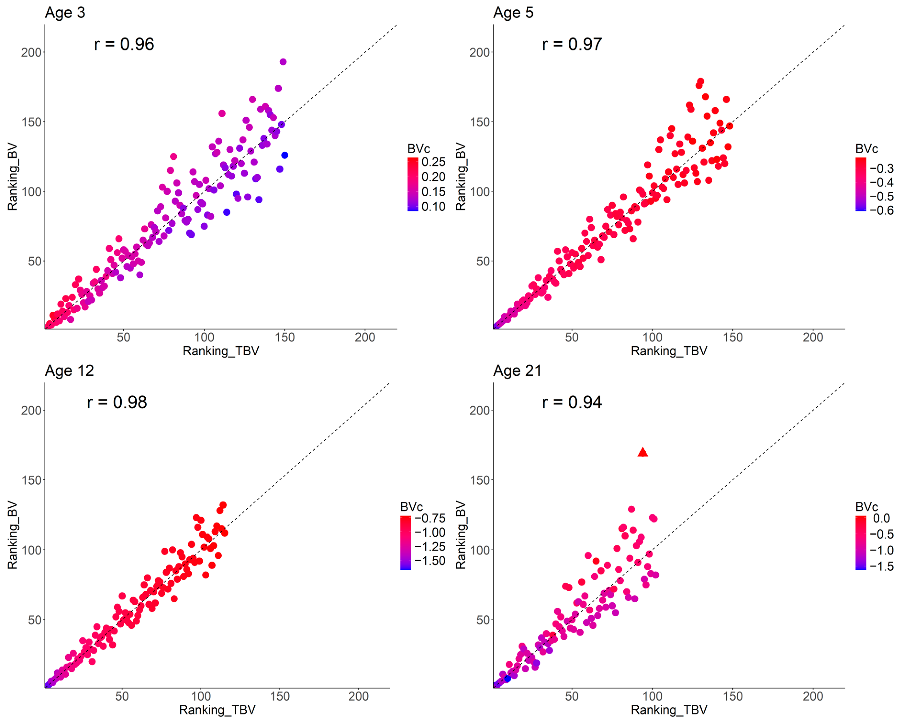
3.4. Breeding Values Accuracy, Response to Selection, and Ranking Changes

Table 6. Mean estimated accuracies for the predicted breeding values ($\mathrm{B}\mathrm{V}\mathrm{s}$) based on the spatial model (Spa), and for the direct breeding values (${\mathrm{B}\mathrm{V}}_{\mathrm{d}}$) and competition breeding values (${\mathrm{B}\mathrm{V}}_{\mathrm{c}}$) from statistically significant (p < 0.05) spatial-competition (Spa-Comp) model across all trait–age combinations at site 1. See text for trait abbreviations.

			$\mathbf{B}\mathbf{V}\left({\mathbf{B}\mathbf{V}}_{\mathit{d}}\right)$		${\mathbf{B}\mathbf{V}}_{\mathbf{c}}$
Trait	Age	Model	Parent	Offspring	Parent	Offspring
	3	Spa	0.79	0.72	-	-
		Spa-Comp	0.79	0.72	0.26	0.15
	5	Spa	0.82	0.80	-	-
		Spa-Comp	0.83	0.81	0.64	0.62
DBH	12	Spa	0.75	0.73	-	-
		Spa-Comp	0.76	0.76	0.75	0.75
	21	Spa	0.68	0.65	-	-
		Spa-Comp	0.67	0.64	0.33	0.27
	3	Spa	0.77	0.68	-	-
		Spa-Comp	0.77	0.69	0.65	0.62
TH	5	Spa	0.82	0.79	-	-
		Spa-Comp	0.82	0.79	0.65	0.64
	5	Spa	0.60	0.48	-	-
		Spa-Comp	0.62	0.51	0.74	0.71
	12	Spa	0.56	0.48	-	-
NSTR		Spa-Comp	0.57	0.49	0.60	0.57
	21	Spa	0.59	0.54	-	-
		Spa-Comp	0.61	0.56	0.38	0.35

presents the average parents’ and offspring’s accuracies for the breeding values (BV) from the Spa model, as well as the direct breeding values (${\mathrm{B}\mathrm{V}}_{\mathrm{d}}$) and competition breeding values (${\mathrm{B}\mathrm{V}}_{\mathrm{c}}$) from the statistically significant (p < 0.05) Spa-Comp model across all trait–age combinations at site 1. As expected, the average accuracy of breeding values for parents was consistently higher than that for offspring, regardless of the model tested. Moreover, the accuracy for both parents and offspring were generally similar or slightly higher with the Spa-Comp compared to the Spa model (i.e., ${\mathrm{B}\mathrm{V}}_{\mathrm{d}}$ vs. BV), with increases ranging from 0.00% to 3.39% for parents and 0.00% to 6.25% for offspring. However, an exception was observed for DBH at age 21, where the Spa model showed slightly higher accuracy for both parents (0.68 vs. 0.67) and offspring (0.65 vs. 0.64) compared to the Spa-Comp model. Additionally, the results from the Spa-Comp model indicated that parents’ and offspring’s accuracies for the ${\mathrm{B}\mathrm{V}}_{\mathrm{d}}$ was generally higher than those estimated for ${\mathrm{B}\mathrm{V}}_{\mathrm{c}}$, except for the NSTR trait at ages 5 and 12. Moreover, while the accuracies of BV and ${\mathrm{B}\mathrm{V}}_{\mathrm{d}}$ for both parents and offspring were generally greater than 0.70, the accuracy values for the NSTR trait were lower than 0.62. Contrarily, the accuracies of ${\mathrm{B}\mathrm{V}}_{\mathrm{c}}$ for all traits were generally lower than 0.70, with the lowest values observed for the DBH trait at age 3, where the parents had an accuracy of 0.26 and the offspring had an accuracy of 0.15.

Table 7. Predicted response to selection ${(\widehat{G}}_s)$ in percentage for all trait–age combinations at site 1, based on the selection of the top 5% offspring according to breeding values (BV) from the spatial model (Spa), and total breeding values (TBVs) from statistically significant (p < 0.05) spatial-competition (Spa-Comp) model. See text for trait abbreviations.

Trait	Age	Model	Criteria	${\widehat{\mathit{G}}}_{\mathit{s}}$	CT%
	3	Spa	BV	18.42
		Spa-Comp	TBV	22.67	93%
	5	Spa	BV	18.62
DBH		Spa-Comp	TBV	14.79	94%
	12	Spa	BV	19.32
		Spa-Comp	TBV	16.26	95%
	21	Spa	BV	16.85
		Spa-Comp	TBV	13.13	89%
	3	Spa	BV	14.15
		Spa-Comp	TBV	13.97	91%
TH	5	Spa	BV	14.15
		Spa-Comp	TBV	15.51	93%
	5	Spa	BV	14.50
		Spa-Comp	TBV	19.52	78%
NSTR	12	Spa	BV	10.60
		Spa-Comp	TBV	7.67	100%
	21	Spa	BV	23.25
		Spa-Comp	TBV	24.48	79%

NOTE: CT%, percentage of common trees selected by both models.

presents the predicted responses to selection (${\widehat{G}}_s$) as percentages for all trait–age combinations at site 1, based on the selection of the top 5% of offspring using the Spa and Spa-Comp models. It also includes the percentage of common trees selected by both models (CT%). Overall, there was a strong agreement in tree selection between the two models across all trait–age combinations (CT% > 79%). However, differences in ${\widehat{G}}_s$ between models across trait–age combinations at site 1 were linked to the relevance of genetic competition (Pearson correlation between ${\widehat{r}}_{a_{dc}}$ and changes in selection response = 0.95; Figure S2), with variations depending on whether competition genetic effects were weak or strong. For DBH, the Spa-Comp model estimated lower ${\widehat{G}}_s$ than the Spa model, except at age 3, where the Spa-Comp model predicted a higher ${\widehat{G}}_s$ (22.67) compared to the Spa model (18.42). At all other ages, the Spa model consistently overestimated ${\widehat{G}}_s$ by approximately 3.06 to 3.83 percentage points compared to the Spa-Comp model. For TH, differences in ${\widehat{G}}_s$ predictions were smaller than those observed for DBH. At age 3, both models produced nearly identical estimates (14.15 for Spa vs. 13.97 for Spa-Comp). At age 5, the Spa-Comp model predicted a slightly higher ${\widehat{G}}_s$ (15.51) compared to the Spa model (14.15). For NSTR, the Spa-Comp model estimated higher ${\widehat{G}}_s$ values at ages 5 (19.52 vs. 14.50 for Spa) and 21 (24.48 vs. 23.25), while the Spa model predicted a higher ${\widehat{G}}_s$ at age 12 (10.60 vs. 7.67 for Spa-Comp).

Figure 2 illustrates the Spearman rank correlations between the offspring BVs predicted by the Spa model and their corresponding TBVs from the Spa-Comp model for the top 5% of selected candidates for DBH trait at site 1. These correlations were consistently high and positive (ranging from 0.94 to 0.98), showing an increasing trend from ages 3 to 12, followed by a slight decline at age 21. The scatter plots further indicate that top-ranked individuals generally maintain their positions regardless of whether the Spa or Spa-Comp model was used, whereas the lower-ranking trees exhibited less stability. Notably, at age 3, the top-ranking trees tend to exhibit lower genetic competition (i.e., those with higher positive ${\mathrm{B}\mathrm{V}}_{\mathrm{c}}$), whereas at more advanced ages (i.e., 5, 12, and 21 years), the top-ranked trees are typically the most competitive (i.e., those with higher negative ${\mathrm{B}\mathrm{V}}_{\mathrm{c}}$). These results highlight that age-related shifts in genetic competition can drive the selection of more aggressive trees. Moreover, at age 3, the right section of the plot illustrates significant fluctuations in the ranking positions of the more competitive trees. Conversely, as trees mature, and genetic competition becomes significant, less competitive trees experience more pronounced changes in their rankings. For instance, at age 21, where 102 trees were selected, one tree ranked 169th based on its BV in the Spa model would have fallen outside the top 5% of selections. However, in the Spa-Comp model, the same tree was ranked 94th based on its TBV, securing its position within the top 5%. This shift is highlighted by the triangular data point in the age 21 plot of Figure 2.

4. Discussion

The primary aim of this study was to investigate the influence of competition on genetic (co)variances in P. taeda trials in Argentina across a range of traits, ages, and sites and to determine the impacts of genetic competition on selection accuracy, response, and ranking changes. Our main results show that across 89 cases (spanning three traits, ages 3 to 21, and 14 test sites), the spatial-competition (Spa-Comp) model was statistically significant in only 27 cases compared to the spatial (Spa) model. The genetic correlations between additive direct and competition effects (${\widehat{r}}_{a_{dc}}$) varied by trait and age, indicating the absence of genetic competition for DBH at age 3, NSTR at age 5, and TH at both evaluated ages (3 and 5). Genetic competition was weak for NSTR at age 21 but strong for DBH from age 5 onward and for NSTR at age 12. The ratio of competition to direct additive genetic variance (${\widehat{\sigma }}_{a_c}^2/{\widehat{\sigma }}_{a_d}^2$) remained below 26% across all trait–age–site combinations, indicating that competition variance was small. When the genetic competition was strong, the negative ${\widehat{r}}_{a_{dc}}$ reduced the total heritable variance (${\widehat{\sigma }}_{TBV}^2$). In this context, the Spa-Comp model showed a slight improvement in breeding value accuracy (<~4%), whereas the Spa model slightly overestimated the selection response for the competition-sensitive trait DBH (<3.83%). Despite this, rank changes were minimal, with most selected trees remaining consistent across both models (>89%), regardless of the trait or age.

4.1. Dynamics of Genetic Competition Across Traits, Ages, and Sites

Negative ${\widehat{r}}_{a_{dc}}$ values for DBH from age 5 onward and across different sites (Table 2) align with previous studies (e.g., [4,9,11,29]), indicating strong genetic competition. In contrast, TH showed consistent positive ${\widehat{r}}_{a_{dc}}$ values (Table 3), suggesting cooperative dynamics. Nagashima and Hikosaka [30] noted that subordinate trees may grow taller while dominant ones reduce growth to match neighbors, influenced by light competition [31] and stability needs [32]. These results highlight the trait-dependent nature of genetic responses (expression) to competition [33]. Gould et al. [34] and Dong et al. [4] suggested that selecting for TH (rather than DBH) may lead to families and individuals with more consistent performance across competitive environments. Genetic competition for NSTR was only significant at site 1 (age 5–21, Table 4), likely due to low precision in its assessment, as it was subjectively scored by different field teams using a four-point or six-point categorical subjective score.

The shift in ${\widehat{r}}_{a_{dc}}$ for DBH from positive at age 3 to negative at age 5 (Table 2) aligns with the negative Pearson correlation coefficients for ${\mathrm{B}\mathrm{V}}_{\mathrm{c}}$ across ages (Table 5), reflecting the transition from non-competitive to competitive interactions as crown closure occurs. At age 3, the absence of branch mortality suggests minimal resource competition, but by age 5, crown closure led to increased shading, reducing DBH growth in smaller trees while benefiting larger ones. Age-specific competition dynamics in P. taeda are consistent with other species, such as the similar shift reported in Pseudotsuga menziesii var. menziesii by Cappa et al. [9] and early intense competition noted in Eucalyptus globulus by Costa e Silva et al. [10]. However, comparing competition genetic effects across ages in tree species is challenging due to variations in measurement timing, environmental factors, and experimental conditions among studies.

The ratio ${\widehat{\sigma }}_{a_c}^2/{\widehat{\sigma }}_{a_d}^2$ ranged between 1 and 26% across all trait–age–site combinations (Table 2, Table 3 and Table 4), consistent with previous studies on forest tree genetic evaluations [4,7,9,10,11,12]. For example, Costa e Silva et al. [10] and Hernández et al. [11] reported low ratios for DBH (<15%) and TH (<19%) in Eucalyptus globulus (ages 2 and 6) and Corymbia citriodora subsp. variegata (F.Muell.) A.R. Bean & M.W. McDonald (age 6), respectively. Similarly, Belaber et al. [12] observed ratios below 11% for growth traits in hybrid pines (Pinus elliottii Engelm. var. elliottii × Pinus caribaea var. hondurensis (Sénécl) Barrett and Golfari) at age 10. Likewise, low ratios were found in Picea abies (1%–9%), while higher ratios were observed in Pinus contorta (24%–31%) and Pinus sylvestris (1%–42%) by Jansson et al. [7]. Additionally, Dong et al. [4] reported a moderate competition-direct variance ratio for TH (17%) at age 20 and a higher ratio for DBH (69%) in Larix kaempferi. Despite being smaller, competition additive genetic variance can significantly contribute to total heritable variation [10].

A high negative genetic covariance between direct and competition effects reduces the ${\widehat{\sigma }}_{TBV}^2$, while a positive covariance increases it. In extreme cases, a negative covariance near −1 can theoretically eliminate total heritable variation [17]. Then, the increase or decrease in ${\widehat{\sigma }}_{TBV}^2$ is associated with the cooperative or competitive nature of the trait being evaluated. In our study, strong genetic competition significantly reduced DBH ${\widehat{\sigma }}_{TBV}^2$ from age 5 onward. Although these reductions lessened with increasing tree age at site 1 (Figure 1), it was less pronounced than expected. This was likely due to stand mortality (22.6% between ages 5 and 12; see Table S1), which reduced the weight of the genetic covariance between direct and competition effects (i.e., $\left({\overline{n}}_R{\overline{f}}_{ijR}+{\overline{n}}_C{\overline{f}}_{ijC}+{\overline{n}}_D{\overline{f}}_{ijD}\right)$) from 2.12 to 1.42, thereby decreasing ${\widehat{\sigma }}_{TBV}^2$. For TH, the absence of genetic competition increased ${\widehat{\sigma }}_{TBV}^2$, while the effects on NSTR varied by ages, increasing the ${\widehat{\sigma }}_{TBV}^2$ at age 5 and 21 but reducing the ${\widehat{\sigma }}_{TBV}^2$ at age 12, associated with a strong genetic competition. These results, showing the impact of varying competition genetic effects on ${\widehat{\sigma }}_{TBV}^2$ across traits and ages, align with Costa e Silva et al. [5] in Eucalyptus globulus. These authors found that ${\widehat{\sigma }}_{TBV}^2$ for the Mycosphaerella leaf disease trait at age 2 exceeded the direct additive genetic variance. In the same study, they found that genetic competition significantly affected ${\widehat{\sigma }}_{TBV}^2$ for DBH between ages 2 and 8, with the impact stabilizing after canopy closure, as indicated by slower changes in genetic parameters for competition effects. They further observed that ${\widehat{\sigma }}_{TBV}^2$ for DBH declined between ages 4 and 8 due to a growing negative genetic covariance between direct and competition effects, despite both genetic variances increasing with stand development.

As expected, we observed varying levels of genetic competition for the same trait and age, influenced by site-specific factors such as soil properties, stand density, and survival rates. For example, higher genetic competition for DBH was seen at sites with favorable growth conditions (e.g., rocky soil at site 10 and clay soil at site 11) (Table 1 and Table S1) where trees were planted at close spacing in at least one direction (2.5 m and 1.8 m, respectively). Increased genetic competition was also noted at site 2, where trees in less favorable conditions were planted at 2.4 × 2.4 m spacing. Despite this variation, few genetic studies have examined competition at the same age and trait under selection in forest species (e.g., [7,8]). Jansson et al. [7] reported ${\widehat{r}}_{a_{dc}}$ values of −0.81 and −0.99 for two Picea abies trials at age 35, while Ferreira et al. [8] observed ${\widehat{r}}_{a_{dc}}$ values of −0.64 and −0.99 for three Eucalyptus dunnii trials across two sites at age 7, suggesting that such differences may stem from environmental variation such as the availability of nutrients and water within the soil. Further research is needed to better understand how site-specific environmental factors and stand characteristics influence genetic competition dynamics, particularly in the context of long-term forest genetic evaluation.

4.2. Impact of Competition Genetic Effects on Theoretical Accuracy, Response to Selection, and Ranking

When environmental variation and inter-tree competition significantly affect forest genetic trials, accounting for both these factors can improve model fit and henceforth, breeding value accuracy [9,13]. While many studies have shown higher theoretical accuracy when comparing spatial models to traditional design-based models (e.g., [23,35,36]), the impact of including competition genetic effects is less obvious. In our study, genetic competition had little effect on breeding value accuracy (i.e., ${\mathrm{B}\mathrm{V}\mathrm{v}\mathrm{s}.\mathrm{B}\mathrm{V}}_{\mathrm{d}}$), with minimal impact on DBH (<4.11%) and NSTR (<3.70%) (Table 6). This aligns with the small differences in additive genetic variance estimates between models (i.e., Spa model, ${\widehat{\sigma }}_a^2$; Spa-Comp model, ${\widehat{\sigma }}_{a_d}^2$) (Table 2, Table 3 and Table 4). Similar results have been reported by Dong et al. [4], who found only slight differences in DBH accuracy (0.37 vs. 0.44) and TH (0.47 vs. 0.49), while Ferreira et al. [6] reported identical volume accuracy (0.96). Overall, once spatial effects were considered, genetic competition improved breeding value accuracy by up to ~4% for DBH and NSTR, the two traits that exhibited genetic competition.

Regarding the response to selection (Table 7), the Spa-Comp model yielded lower ${\widehat{G}}_s$ than the Spa model when the genetic competition was strong, but higher ${\widehat{G}}_s$ when competition was weak or absent (see also Figure S2). Therefore, excluding genetic competition led to slight overestimations of the genetic gains for DBH (up to 3.8 percentage points) and underestimations for NSTR (up to 5.0 percentage points), while the impact on TH was minimal, as tree height is generally less influenced by competition genetic effects. These results underscore the limitations of the simple Spa model in the presence of strong genetic competition. This aligns with the findings of Costa e Silva and Kerr [18], based on simulations, and Costa e Silva et al. [5], who analyzed empirical data on DBH trait in Eucalyptus globulus. However, empirical studies show mixed results on the impact of accounting for genetic competition in DBH selection models. Hernández et al. [11] reported a 13.5 percentages point increase in selection response at age 6 in Corymbia citriodora subsp. variegata, while Dong et al. [4] observed a ~27% reduction at age 20 in Larix kaempferi. These findings emphasize that the effects of genetic competition on the responses to selection should be evaluated for competition-sensitive traits like DBH.

While selecting based on ${\mathrm{B}\mathrm{V}}_{\mathrm{d}}$ can maximize genetic gain, implementing thinning regimes to manage tree density is crucial to mitigate competition genetic effects [4]. However, selecting non-competitive genotypes may lead to the greatest yields per unit area, aligning with the ‘crop ideotype’ concept [37]. In this sense, selecting individuals based on TBVs, as suggested by Costa e Silva and Kerr [18], may enhance overall stand productivity, particularly in low-maintenance plantations, where deploying trees with high ${\mathrm{B}\mathrm{V}}_{\mathrm{d}}$ but low competition effects can optimize genetic gains [4].

In this breeding strategy, selecting trees with high ${\mathrm{B}\mathrm{V}}_{\mathrm{d}}$ but low competition genetic effects is crucial for enhancing overall stand productivity while minimizing the suppression of neighboring trees. In our P. taeda datasets, competition genetic effects became more pronounced from age 5, with faster-growing trees exerting stronger competitive pressures (Figure 2). However, as noted by Dong et al. [4], the strong negative correlation between ${\mathrm{B}\mathrm{V}}_{\mathrm{d}}$ and ${\mathrm{B}\mathrm{V}}_{\mathrm{c}}$ presents a significant challenge for selection. For instance, at ages 5 and 12, the ${\widehat{r}}_{a_{dc}}$ for DBH at site 1 was highly negative (−0.81 and −0.98, respectively; Table 2), making it difficult to identify trees that exhibit both strong direct genetic effects (high positive direct breeding values) and minimal competition genetic effects (low negative competition breeding values) (Figure S3). By age 21, however, this correlation declined to −0.52 (Table 2), suggesting the potential to identify trees with both improved growth and reduced competition genetic effects. The shift from positive to negative correlation between ${\mathrm{B}\mathrm{V}}_{\mathrm{d}}$ and ${\mathrm{B}\mathrm{V}}_{\mathrm{c}}$ around age 4 (0.51 at age 3 to −0.81 at age 5) indicates a transition from symmetric to asymmetric competition (see comment below), marking a critical window for the selection of trees with both favorable direct genetic effects and reduced competition genetic effects. This transition is influenced by site productivity, stand density, and survival rates, which can impact the timing and intensity of competition effects. Identifying trees that balance high individual productivity with minimal competitive impact during this early phase may optimize genetic gains while maintaining stand-level performance. These findings highlight the importance of considering the temporal dynamics of genetic competition when designing selection strategies for long-lived species such as P. taeda.

The ranking of selected candidates remained highly consistent between BV from the Spa model and TBV from the Spa-Comp model for DBH at site 1 across ages 3 to 21, despite some strongly negative ${\widehat{r}}_{a_{dc}}$ (Table 2). High Spearman correlations (>0.94; Figure 2) indicate minimal ranking shifts regardless of genetic competition. Simulations by Costa e Silva and Kerr [18] demonstrated that ranking alignment between BV from standard and TBV from spatial-competition models declined as ${\widehat{r}}_{a_{dc}}$ became more negative and/or ${\widehat{\sigma }}_{a_c}^2$ increased. They showed that when the ${\widehat{\sigma }}_{a_c}^2/{\widehat{\sigma }}_{a_d}^2$ ratio was 10%, the Spearman coefficient remained at 0.793 for ${\widehat{r}}_{a_{dc}}$ values of −0.30 and −0.90 (common selected trees 63/130 and 51/130, respectively). However, at a 50% ratio, it dropped to 0.210 for ${\widehat{r}}_{a_{dc}}$ = −0.30 (common selected trees 11/130) and to −0.765 for ${\widehat{r}}_{a_{dc}}$ = −0.90 (common selected trees 0/130). In our study, this ratio remained below 10%, with ${\widehat{r}}_{a_{dc}}$ ranging from −0.52 to −0.98, which may explain the observed ranking stability. Competition genetic effects on tree rankings have been documented in both empirical [7,9,12,38] and simulated studies [18]. Our findings align with Jansson et al. [7], who reported minimal ranking changes for DBH due to low competition additive genetic variance. However, other studies found stronger impacts for DBH. For instance, Cappa et al. [9] reported moderate to high Spearman correlations (>0.58) with notable differences in top selections, while Belaber et al. [12] observed moderate correlations (0.71) and divergent selection outcomes.

Finally, our study shows that across all ages, trees with greater DBH growth maintain more stable rankings between the Spa and Spa-Comp models, while smaller trees experience greater rank variation, indicating a stronger impact of genetic competition on predicting breeding values for smaller trees compared to larger ones (Figure 2). An interesting observation at age 3 is that top-ranking trees were less competitive (more positive ${\mathrm{B}\mathrm{V}}_{\mathrm{c}}$, red in Figure 2), but from age 5 onward, they became more competitive (with more negative ${\mathrm{B}\mathrm{V}}_{\mathrm{c}}$, blue in Figure 2). This shift aligns with competition dynamics in forest stands. Binkley [39] suggested that before canopy closure, all trees use resources efficiently, but post-closure, dominance reduces efficiency for subordinates. Fernández and Gyenge [40], testing Binkley’s hypothesis in Pinus ponderosa Douglas ex C. Lawson stands, suggested that resource-use efficiency differences can emerge before dominance, driving variations in size and social position. As trees grow and access more resources, their efficiency improves but declines as resources become limited due to competition or environmental stress. West [41] described competition as symmetric (growth proportional to size) or asymmetric (larger trees gain disproportionate advantages). Initially, seedlings compete symmetrically for water and nutrients, but as they grow, height differences lead to asymmetric competition for sunlight, with taller trees shading smaller ones and intensifying the competition for both light and other resources. In our study, symmetric below-ground competition until age 3 (prior to canopy closure) may explain the positive influence of genetic competition on DBH, with top-ranking trees being less competitive. After canopy closure (age 5 onward), asymmetric light competition (post canopy closure) likely drove the negative influence of genetic competition on the DBH trait (Table 2), resulting in top-ranking trees exhibiting strong competition genetic effects (Figure 2).

5. Conclusions

This study investigated the influence of genetic competition on growth and stem straightness traits in P. taeda across diverse ages and site conditions, confirming that diameter at breast height (DBH) is the most competition-sensitive trait, while total height (TH) and stem straightness (NSTR) are less affected. However, these competition genetic effects change with age and site. At younger ages, trees with higher genetic merit for growth tend to be less competitive. From age 5 onward, trees with higher genetic merit are associated with higher competition genetic effects. The presence of genetic competition effects and the strongly negative genetic covariance between competition and direct effects, resulted in a significant reduction in the total genetic variance for growth. This shift suggests that selection may increasingly favor aggressive competitors, shaping long-term breeding outcomes.

While ignoring competition genetic effects did not significantly alter selection rankings or breeding value accuracy, its impact on total genetic response could, therefore, be relevant, biasing the genetic gain in DBH by up to ~4 percentage points in extreme cases (e.g., from 16.85 to 13.13 at age 21). These findings emphasize the need to include genetic competition in breeding models although the magnitude of such effects will depend on the trait, age, and the specific site conditions under which breeding evaluations are conducted. Future studies should examine how genetic competition affects other key traits, such as wood density in P. taeda. More competitive trees may exhibit lower wood density due to accelerated growth, while less competitive trees could yield higher-density wood, benefiting industries such as construction. Understanding these genetic trade-offs will help optimize breeding strategies to balance growth and wood quality for specific industrial needs.

References

1. Cappa, E.P.; Cantet, R.J.C. Direct and Competition Additive Effects in Tree Breeding: Bayesian Estimation From an Individual Tree Mixed Model. Silvae Genet. 2008, 57, 45–56. [Google Scholar] [CrossRef]
2. Shalizi, M.N.; McKeand, S.E.; Walker, T.D. Age Affects Genetic Gain Estimates in Pinus taeda L. Progeny Tests. Silvae Genet. 2024, 73, 149–159. [Google Scholar] [CrossRef]
3. Brotherstone, S.; White, I.M.S.; Sykes, R.; Thompson, R.; Connolly, T.; Lee, S.; Woolliams, J. Competition Effects in a Young Sitka Spruce (Picea sitchensis, Bong. Carr) Clonal Trial. Silvae Genet. 2011, 60, 149–155. [Google Scholar] [CrossRef]
4. Dong, L.; Xie, Y.; Wu, H.X.; Sun, X. Spatial and Competition Models Increase the Progeny Testing Efficiency of Japanese Larch. Can. J. For. Res. 2020, 50, 1373–1382. [Google Scholar] [CrossRef]
5. Costa e Silva, J.; Potts, B.M.; Gilmour, A.R.; Kerr, R.J. Genetic-Based Interactions among Tree Neighbors: Identification of the Most Influential Neighbors, and Estimation of Correlations among Direct and Indirect Genetic Effects for Leaf Disease and Growth in Eucalyptus Globulus. Heredity 2017, 119, 125–135. [Google Scholar] [CrossRef]
6. Ferreira, F.M.; Chaves, S.F.S.; Bhering, L.L.; Alves, R.S.; Takahashi, E.K.; Sousa, J.E.; Resende, M.D.V.; Leite, F.P.; Gezan, S.A.; Viana, J.M.S.; et al. A Novel Strategy to Predict Clonal Composites by Jointly Modeling Spatial Variation and Genetic Competition. For. Ecol. Manag. 2023, 548, 121393. [Google Scholar] [CrossRef]
7. Jansson, G.; Kerr, R.; Dutkowski, G.; Kroon, J. Competition Effects in Breeding Value Prediction of Forest Trees. Can. J. For. Res. 2021, 51, 1002–1014. [Google Scholar] [CrossRef]
8. Ferreira, F.M.; Chaves, S.F.D.S.; Dos Santos, O.P.; Nunes, A.C.P.; Tambarussi, E.V.; Pereira, G.D.S.; Dos Santos, G.A.; Bhering, L.L.; Dias, K.O.D.G. Competition Effects Can Mislead Selection in Eucalypt Breeding Trials. For. Ecol. Manag. 2024, 561, 121892. [Google Scholar] [CrossRef]
9. Cappa, E.P.; Stoehr, M.U.; Xie, C.-Y.; Yanchuk, A.D. Identification and Joint Modeling of Competition Effects and Environmental Heterogeneity in Three Douglas-Fir (Pseudotsuga menziesii Var. Menziesii) Trials. Tree Genet. Genomes 2016, 12, 102. [Google Scholar] [CrossRef]
10. Costa e Silva, J.; Potts, B.M.; Bijma, P.; Kerr, R.J.; Pilbeam, D.J. Genetic Control of Interactions among Individuals: Contrasting Outcomes of Indirect Genetic Effects Arising from Neighbour Disease Infection and Competition in a Forest Tree. New Phytol. 2013, 197, 631–641. [Google Scholar] [CrossRef]
11. Hernández, M.A.; López, J.A.; Cappa, E.P. Improving Genetic Analysis of Corymbia Citriodora Subsp. Variegata with Single- and Multiple-Trait Spatial-Competition Models. For. Sci. 2019, 65, 570–580. [Google Scholar] [CrossRef]
12. Belaber, E.C.; Gauchat, M.E.; Schoffen, C.D.; Muñoz, F.; Borralho, N.M.; Sanchez, L.; Cappa, E.P. Accounting for Competition in Multi-Environment Tree Genetic Evaluations: A Case Study with Hybrid Pines. Ann. For. Sci. 2021, 78, 2. [Google Scholar] [CrossRef]
13. de Araujo, M.J.; da Rocha, G.N.; Estopa, R.A.; Oberschelp, J.; da Silva, P.H.M. Conservative or Non-Conservative Strategy to Advance Breeding Generation? A Case Study in Eucalyptus benthamii Using Spatial Variation and Competition Model. Silvae Genet. 2023, 72, 1–10. [Google Scholar] [CrossRef]
14. Baud, A.; McPeek, S.; Chen, N.; Hughes, K.A. Indirect Genetic Effects: A Cross-Disciplinary Perspective on Empirical Studies. J. Hered. 2022, 113, 1–15. [Google Scholar] [CrossRef] [PubMed]
15. Flores Junior, P.C.; Ishibashi, V.; Matos, J.L.M.D.; Martinez, D.T.; Higa, A.R. Effect of Competition in Different Ages in a Progeny Test of Pinus taeda L. Sci. For. 2020, 48, e3290. [Google Scholar] [CrossRef]
16. Ishibashi, V.; Martinez, D.T.; Higa, A.R. Phenotypic Models of Competition for Pinus taeda L Genetic Parameters Estimation. CERNE 2017, 23, 349–358. [Google Scholar] [CrossRef]
17. Bijma, P. A General Definition of the Heritable Variation That Determines the Potential of a Population to Respond to Selection. Genetics 2011, 189, 1347–1359. [Google Scholar] [CrossRef]
18. Costa e Silva, J.; Kerr, R.J. Accounting for Competition in Genetic Analysis, with Particular Emphasis on Forest Genetic Trials. Tree Genet. Genomes 2013, 9, 1–17. [Google Scholar] [CrossRef]
19. Cadena de Valor Foresto Industrial–Producción Foresto Industrial. Available online: https://www.magyp.gob.ar/desarrollo-foresto-industrial/cadena-valor.php (accessed on 21 March 2025).
20. Gianola, D.; Norton, H.W. Scaling Threshold Characters. Genetics 1981, 99, 357–364. [Google Scholar] [CrossRef]
21. Henderson, C.R. Applications of Linear Models in Animal Breeding; University of Guelph: Guelph, ON, Canada, 1984. [Google Scholar]
22. Gilmour, A.R.; Cullis, B.R.; Verbyla, A.P.; Verbyla, A.P. Accounting for Natural and Extraneous Variation in the Analysis of Field Experiments. J. Agric. Biol. Environ. Stat. 1997, 2, 269. [Google Scholar] [CrossRef]
23. Dutkowski, G.W.; Silva, J.C.E.; Gilmour, A.R.; Lopez, G.A. Spatial Analysis Methods for Forest Genetic Trials. Can. J. For. Res. 2002, 32, 2201–2214. [Google Scholar] [CrossRef]
24. Gilmour, A.R.; Thompson, R.; Cullis, B.R. Average Information REML: An Efficient Algorithm for Variance Parameter Estimation in Linear Mixed Models. Biometrics 1995, 51, 1440–1450. [Google Scholar] [CrossRef]
25. R Core Team. R: A Language and Environment for Statistical Computing; R Foundation for Statistical Computing: Vienna, Austria, 2022; Available online: https://www.bibsonomy.org/bibtex/7469ffee3b07f9167cf47e7555041ee7 (accessed on 24 March 2025).
26. Butler, D.G.; Cullis, B.R.; Gilmour, A.R.; Gogel, B.J.; Thompson, R. ASReml-R Reference Manual Version 4.2; VSN International Ltd.: Hemel Hempstead, UK, 2023. [Google Scholar]
27. Wickham, H. Ggplot2: Elegant Graphics for Data Analysis, Use R! 2nd ed.; Springer International Publishing: Cham, Switzerland, 2016; ISBN 978-3-319-24275-0. [Google Scholar]
28. Stram, D.O.; Lee, J.W. Variance Components Testing in the Longitudinal Mixed Effects Model. Biometrics 1994, 50, 1171. [Google Scholar] [CrossRef]
29. de Araujo, M.J.; de Paula, R.C.; de Moraes, C.B.; Pieroni, G.; da Silva, P.H.M. Thinning Strategies for Eucalyptus Dunnii Population: Balance between Breeding and Conservation Using Spatial Variation and Competition Model. Tree Genet. Genomes 2021, 17, 42. [Google Scholar] [CrossRef]
30. Nagashima, H.; Hikosaka, K. Plants in a Crowded Stand Regulate Their Height Growth so as to Maintain Similar Heights to Neighbours Even When They Have Potential Advantages in Height Growth. Ann. Bot. 2011, 108, 207–214. [Google Scholar] [CrossRef]
31. Bergmüller, K.O.; Vanderwel, M.C. Evaluating Effects of Remotely Sensed Neighborhood Crowding and Depth-to-Water on Tree Height Growth. Forests 2023, 14, 242. [Google Scholar] [CrossRef]
32. Meng, S.X.; Lieffers, V.J.; Reid, D.E.B.; Rudnicki, M.; Silins, U.; Jin, M. Reducing Stem Bending Increases the Height Growth of Tall Pines. J. Exp. Bot. 2006, 57, 3175–3182. [Google Scholar] [CrossRef]
33. von Euler, F.; Baradat, P.; Lemoine, B. Effects of Plantation Density and Spacing on Competitive Interactions among Half-Sib Families of Maritime Pine. Can. J. For. Res. 1992, 22, 482–489. [Google Scholar] [CrossRef]
34. Gould, P.J.; Clair, J.B.S.; Anderson, P.D. Performance of Full-Sib Families of Douglas-Fir in Pure-Family and Mixed-Family Deployments. For. Ecol. Manag. 2011, 262, 1417–1425. [Google Scholar] [CrossRef]
35. Ye, T.Z.; Jayawickrama, K.J.S. Efficiency of Using Spatial Analysis in First-Generation Coastal Douglas-Fir Progeny Tests in the US Pacific Northwest. Tree Genet. Genomes 2008, 4, 677–692. [Google Scholar] [CrossRef]
36. Chen, Z.; Helmersson, A.; Westin, J.; Karlsson, B.; Wu, H.X. Efficiency of Using Spatial Analysis for Norway Spruce Progeny Tests in Sweden. Ann. For. Sci. 2018, 75, 2. [Google Scholar] [CrossRef]
37. White, T.L.; Adams, W.T.; Neale, D.B. Forest Genetics, 1st ed.; CABI: Wallingford, UK, 2007; ISBN 978-0-85199-348-5. [Google Scholar]
38. Chaves, S.F.S.; Ferreira, F.M.; Ferreira, G.C.; Gezan, S.A.; Dias, K.O.G. Incorporating Spatial and Genetic Competition into Breeding Pipelines with the R Package Gencomp. Heredity 2025, 134, 129–141. [Google Scholar] [CrossRef] [PubMed]
39. Binkley, D. A Hypothesis about the Interaction of Tree Dominance and Stand Production through Stand Development. For. Ecol. Manag. 2004, 190, 265–271. [Google Scholar] [CrossRef]
40. Fernández, M.E.; Gyenge, J. Testing Binkley’s Hypothesis about the Interaction of Individual Tree Water Use Efficiency and Growth Efficiency with Dominance Patterns in Open and Close Canopy Stands. For. Ecol. Manag. 2009, 257, 1859–1865. [Google Scholar] [CrossRef]
41. West, P.W. Quantifying Effects on Tree Growth Rates of Symmetric and Asymmetric Inter-Tree Competition in Even-Aged, Monoculture Eucalyptus Pilularis Forests. Trees 2023, 37, 239–254. [Google Scholar] [CrossRef]
Figure 1. Mean relative contributions of the variances of direct and competition genetic effects, as well as their covariance (direct-competition genetic covariance), to the total heritable variance for all traits and ages evaluated, expressed as a proportion of the phenotypic variance. The traits diameter at breast height (DBH), total tree height (TH), and the normal score for stem straightness (NSTR) are followed by a number denoting the age of measurement in years. Results are based on all statistically significant (p < 0.05) spatial-competition (Spa-Comp) models. Error bars represent mean standard errors, and mean contributions are shown above each bar.
Forests 16 00675 g001
Figure 2. Scatter plot of the ranking for the top 5% offspring trees selected at ages 3, 5, 12, and 21 based on breeding values ( B V ) from the spatial model (Spa) and total breeding values ( T B V ) from the spatial-competition (Spa-Comp) model, for DBH at site 1. The most competitive trees (i.e., those with highest negative competition breeding values; B V c ) are highlighted in blue and those less competitive in red. Spearman rank correlation is in the left corner of each plot. At age 21, the triangle represents a tree that would not rank among the top 5% of selected trees based on the BV from the Spa model but would be included based on its TBV from the Spa-Comp model.
Forests 16 00675 g002