Evaluation of Landscape Soil Quality in Different Types of Pisha Sandstone Areas on Loess Plateau

Abstract

Severe soil erosion and land productivity degradation caused by inadequate vegetation cover pose significant challenges to regional ecological protection and sustainable development. To assess changes and variations in soil quality, three sample areas with different distinct texture characteristics were selected from the Pisha sandstone region located northeastern of the Loess Plateau. The total data set (TDS) was determined through sampling experiments, and the minimum data set (MDS) was established using principal component analysis. A Random Forest (RF) machine learning model was applied to predict soil quality distribution. The prediction indices were derived from soil analysis dimensions, mean weight diameter measured via wet sieving, and soil enrichment ratio obtained from slope erosion experiments conducted at the corresponding sampling points. During the RF modeling process, 80% of the total soil quality index (SQI), calculated using TDS and MDS evaluation methods, was allocated for model training. The results indicated that pH, ammonia nitrogen, bulk density, silt content, clay content, soil water content, hygroscopic water content, total phosphorus, soluble calcium, and actinomycetes were identified as the optimal predictors for SQI. Furthermore, the RF model demonstrated superior performance in predicting the regional distribution of SQI, with evaluation metrics including (R² = 0.76–0.78, RMSE = 0.03–0.06, MAE = 0.04–0.09). This study confirms the reliability of RF in simulating SQI within the study area and highlights that, in regions undergoing extensive vegetation restoration and with limited sampling conditions, experimental measurements of soil particles and sediment parameters provide an effective approach for evaluating SQI.

1. Introduction

Under the combined effects of climate change and unsustainable human activities, land degradation has emerged as a critical global issue [1,2,3]. In parallel, the degradation of soil quality has attracted widespread attention due to its significant implications for ecosystem health and productivity [4,5]. Soil quality (SQ) serves as an essential indicator of changes in soil structure and the effectiveness of soil management practices. Evaluating soil quality provides insights into the dynamic state of the soil, aiding in understanding the ecological impact of vegetation restoration and enhancing strategies for soil erosion control. As a vital component of healthy ecosystems, soil quality reflects the soil’s overall capacity to sustain ecological functions. It is an important parameter for assessing the soil’s ability to support vegetation growth and understanding the potential and variability of ecosystem services and their associated values [6,7,8]. Evaluating soil quality is, therefore, crucial for addressing issues of land degradation and guiding efforts in regional ecological restoration. Various methods have been developed to assess soil quality, including the soil quality index (SQI) method, the Soil Management Evaluation Framework (SMEF), the Fuzzy Association Rule (FAR) method, etc. Among them, the soil quality index (SQI) approach is widely adopted due to its intuitive nature and flexibility in practical applications [9,10,11,12,13]. The SQI method enables a more comprehensive and accessible evaluation of soil quality by integrating multiple soil properties into a single index, facilitating its use across different research contexts and management scenarios.

At present, the evaluation work based on the soil quality index method mainly follows the following steps: (1) select the appropriate soil property index and SQI type; (2) convert the scores of various soil indexes; (3) according to the integration method of SQI, all index scores are merged. Therefore, selecting suitable soil property indexes to compose suitable total data sets (TDSs) is a key step in the evaluation process. The index composition of TDS is relatively detailed and can reflect various properties of the soil under study as much as possible, but at the same time, there are also problems of information redundancy and duplication among TDS indicators [7,9], in addition to increasing the cost, more soil index measurement will also increase the probability of large errors and uncertainties in the test, which will affect the subsequent evaluation process. The evaluation of SQ should focus on deleting and retaining the minimum data set (MDS) of valid soil property indicators to improve the evaluation efficiency and enhance the effectiveness of vegetation restoration [7,14]. In order to fully reflect the status and differences of soil quality, soil property indicators constituting MDS should have the following characteristics [7,15]: (1) a good indicator of soil basic properties, ecosystem service functions, and soil degradation; (2) ideal test results can be obtained through mature and universal measurement methods for soil indexes; (3) the difference of opposite land types and vegetation restoration measures are more sensitive, and the spatiotemporal variability is as little as possible. The applicability of MDS often depends on the soil structure characteristics, management measures, and regional climate characteristics of the study area [16].

The Pisha sandstone area is located in the upper and middle reaches of the Yellow River, at the junction of Shanxi, Shaanxi, and the Mongolian Autonomous Region. The Pisha sandstone is characterized by its low rock formation degree and weak structural strength. When dry, it forms a hard surface, but it becomes soft when in contact with water, making it highly susceptible to erosion from external forces. The concentration of summer precipitation in the Pisha sandstone distribution area, coupled with the long-term lack of vegetation cover, makes it one of the regions with the highest annual soil erosion modulus on the Loess Plateau, as well as a significant source of coarse sediment in the middle reaches of the Yellow River. Based on different soil texture characteristics, the Pisha sandstone area can be categorized into three regions: the Typical Pisha sandstone area (PSA), aeolian soil area (ASA), and Loess soil area (LSA). The significant differences in soil particle composition across these regions lead to notable variations in their erosion characteristics. The highest erosion modulus and gully density are found in the Typical Pisha Sandstone area, followed by the aeolian soil area, while the Loess soil area experiences relatively lower erosion. These differences in erosion dynamics have been well-documented in previous studies [17].

In recent years, there have been significant research contributions on soil erosion and ecological management in the Pisha sandstone area, with a focus on vegetation restoration [18], soil water infiltration [19], and erosion characteristics [20,21]. Previous studies have focused on the improvement and utilization of soil in the Pisha sandstone area [22,23,24], as well as on research concerning individual indicators of soil moisture or single-sort elements [25,26], studies specifically addressing soil quality evaluation across different Pisha sandstone types are relatively scarce. Therefore, we hypothesized that there was an alternative statistical difference between TDS and MDS and constructed a data set with appropriate indicators based on the physical, chemical, and biological properties of surface soils in different Pisha sandstone types. Our research provides a more specific understanding of soil properties across different types of regions in the Pisha sandstone area and a reference for ecological restoration and construction in such regions.

2. Materials and Methods

2.1. Study Region

The study was conducted in Junger Banner County and Shenmu County, which are located in Ordos City and Yulin City, respectively, in the northern Loess Plateau region (39°26′–39°56′ N,110°32′–111°06′ E), Inner Mongolia and Shaanxi Province, China. The study area lies at an elevation of 800–1500 m above sea level and experiences a temperate continental monsoon climate. The average annual temperature ranges from 8.9 °C to 10 °C, while the average annual precipitation is approximately 400.7 mm, with rainfall concentrated in July, August, and September, accounting for 70% of the annual total. The potential annual evaporation is estimated at 1800–2000 mm. The region is characterized by an average wind speed of about 3 m·s⁻¹ and more than 30 days of strong winds per year. These climatic factors contribute to widespread wind erosion of landforms, loose soil structures, and weak resistance to external impacts and cohesion in the area [27] (Figure 1).

2.2. Soil Sampling Design

All sampling sites were selected as representative sites typical in the study area, with their basic characteristics summarized in

Table 1. Situations of sampling sites in distribution areas of different Pisha sandstone types.

Sample Plots Location	Plot Classification	Longitude and Latitude	Number of Points
Nuanshui	Typical Pisha Sandstone area (PSA)	39°47′15″ N 110°35′54″ E	34
Tetong Gully		39°47′19″ N 110°36′4″ E	12
Shibu Ertai Gully		39°59′58″ N 109°53′36″ E	80
Er Laohu Gully	Loess soil area (LSA)	39°47′40″ N 110°36′7″ E	164
Tela Gully	Aeolian soil area (ASA)	39°34′6″ N 110°57′34″ E	72
Ada Freeway		39°27′50″ N 109°56′59″ E	20
Huojitu		39°14′12″ N 110°10′13″ E	20
Hala Gully		39°31′68″ N 110°21′6″ E	20
Shigetai Gully		39°41′45″ N 110°8′12″ E	20

. To account for the variability in catchment characteristics and basin length across the study area, the sampling process followed the principle of minimizing standard deviation in data analysis. Consequently, each basin was divided into distinct sampling intervals based on these differences. During sampling, each cross section was divided into five sampling points: the top of the sunny and sandy slope, the middle of the sunny and sandy slope, half the height of each cross section, and the bottom of the trench. Soil samples were collected from the 0–20 cm soil layer, spanning from the top to the bottom. During the sample sites and vegetation survey, sampling points within the basins were used as centers for laying out 5 m × 5 m quadrats. Each quadrat was further subdivided into smaller 1 m × 1 m subplots located at the four corners and the center of the quadrat. Within each subplot, the names of the vegetation species, the number of species present, and the vegetation coverage within the subplots were recorded. Meanwhile, soil samples were collected from five different subplots within each quadrat and then thoroughly mixed to ensure distribution.

2.3. Soil Property Analysis

The soil property parameters selected for evaluation must be highly sensitive and representative of functional changes in soil caused by soil and water conservation measures [28,29]. In this study, the soil’s physical and chemical property parameters were relatively stable over short time periods, while biological property parameters were highly sensitive to environmental changes. Although measuring soil biological indicators was often labor-intensive and time-consuming, they provided critical insights into variations in soil quality and the effectiveness of different treatment strategies.

To ensure comprehensive soil quality (SQ) evaluation within the constraints of experimental conditions, soil physical and chemical property parameters were prioritized as the primary indices in this study. Additionally, the soil’s biological property parameters were included to enhance the evaluation framework and provide a more detailed understanding of the impact of soil and water conservation measures. The laboratory tests encompassed the measurement of the soil’s physical, chemical, and biological properties, and the indicators contained physical characters [30], available nutrients [31], soil microbial quantity [32], and soil AM fungal spore diversity [33] (

Table 2. Soil indices and testing methods involved in this study.

Categories of Indicator	Indicators and Abbreviation	Test Method and Devices
Physical	Soil water content (SWC), hygroscopic water content (Wh), bulk density (BD), soil particle composition	Drying–weighing method
Chemical	pH	Mettler–Toledo testing
	Organic carbon (OC)	Potassium dichromate-concentrated sulfuric acid external heating
	Total nitrogen (TN)	Elementar vario MACROCUBE elemental analyzer
	Ammonia nitrogen, available (AN) available phosphorus (AP), available potassium (AK)	Top-cloud TPY-6PC soil nutrient rapid measurement
	Total phosphorus (TP)	NaOH melt-molybdenum reaction colorimetric
	Soluble calcium (Ca)	Atomic absorption spectroscopy
	Nitrate (Ni)	Reduction distillation
	Total potassium (TK)	Alkali fusion
Biological	Culturable fungi (Fu), culturable bacteria (Ba), and culturable actinomycetes (AC)	Microbial medium and pipetting
	Activities of alkaline phosphatase (AKP), acid phosphatase (ACP), neutral phosphatase (NP)	0.5% phenylene disodium phosphate
	Activities of urease (URE), invertase (SC), and catalase (CAT)	Modified indophenol blue colorimetric method, phthalic acid buffer method, and potassium permanganate titration method
	Spore density (SD), spore richness (SRS), Shannon–Wiener index (SWI), and Simpson index (SI)	Wet sieve pour and sucrose centrifugation (50 g of soil as the standard sample size)

).

The soil particle composition exhibited significant variations across the study area. To characterize soil particle composition, enrichment rate (ER), fractal dimension (D), and mean weight diameter (MWD) were employed. The determination of ER and fractal dimension (D) involved a combination of wet and dry screening methods alongside laser dynamic analysis. The experimental steps were as follows: (1) A 30 g soil sample was used as the unit mass. The sample was soaked for over 12 h and subsequently boiled for 1 h to ensure thorough dispersion of the soil particles. (2) The dispersed soil sample was passed through a 0.075 mm soil screen. Soil particles larger than 0.075 mm were collected, dried, and successively sieved using fine mesh screens with aperture sizes of 2 mm, 1 mm, 0.5 mm, 0.25 mm, 0.1 mm, and 0.075 mm. The cumulative sieve components were recorded during this process. (3) The particle size distribution of soil particles smaller than 0.075 mm (post-washing and sieving) was determined using the Malvern Mastersizer 2000 laser particle size analyzer (Malvern Instruments, Malvern, UK).

$$\mathit{ER}={\displaystyle \frac{P_i}{P_0}}$$

(1)

where $P_i$ refers to the volume percentage (%) of soil particles in the erosion in a certain particle size range; $P_0$ represents the percentage of the volume of particles in the undisturbed soil sample (%).

$${\left({\displaystyle \frac{\overline{d_i}}{\overline{d_{\max }}}}\right)}^{3-D}={\displaystyle \frac{V(\delta <\overline{d_i})}{V_0}}$$

(2)

$$D=3-\mathit{lg}\left({\displaystyle \frac{V\left(\delta <\overline{d_i}\right)}{V_0}}\right)/\mathit{lg}\left({\displaystyle \frac{\overline{d_i}}{\overline{d_{\mathit{max}}}}}\right)$$

(3)

where $\overline{d_i}$ indicates the average particle size between ($d_i$ and $d_{i+1}$) (i = 1, 2, 3 …, $d_i$ > $d_{i+1}$), (mm); $\overline{d_{\max }}$ indicates the average particle size between the two groups of maximum particle sizes (mm). $V\left(\delta <\overline{d_i}\right)$ represents the cumulative volume of particles with a particle size smaller than $d_i$; $V_0$ is the sum of the volumes of a single particle size.

The wet sieving method was employed to determine the mean weight diameter (MWD) of soil particles. The experimental procedure was outlined as follows: (1) The soil sample was first passed through an 8 mm soil screen to remove larger particles. The remaining soil was dried and then placed in a 250 μm sieve. (2) The soil on the 250 μm screen was soaked in distilled water for 5 min. The sieve was then moved up and down 10 times, each time covering a distance of 3 cm. This process lasted for 2 min. (3) The soil particles and water that passed through the 250 μm sieve were poured onto a 53 μm sieve. Similar to the previous step, the sieve was moved up and down 10 times, each time covering a distance of 3 cm but with a duration of 3 min. Both the soil particles retained on the sieve and those suspended in the water column were collected for further analysis. (4) The soil particles collected from each sieve were dried at 40 °C and then weighed. The mass distribution of soil particles across different size ranges was recorded.

$$\mathit{MWD} =\sum _{i=1}^3 {\displaystyle \frac{x_{i-1}+x_i}{2}}·{\omega }_i$$

(4)

where i represents the 3 particle sizes selected during the experiment, and $x_i$ represents the average weight diameter of the i th grade (i = 1, 2, 3, mm). When i = 1, $x_{i-1}$ = $x_i$; ${\omega }_i$ represents the mass percentage of grade i th particles (%).

2.4. Data Filtration and Treatment

2.4.1. Establishing Minimum Datasets

Calculating the SQI is essential for providing a theoretical reference for understanding the current state of soil quality and for developing effective ecological restoration strategies [34,35]. The appropriate selection of soil quality indicators played a crucial role in ensuring the accuracy and reliability of soil quality assessments. A key step in the evaluation process involved constructing MDS, which is derived from TDS and includes only the most relevant soil indicators suitable for the specific characteristics of different regions [36,37,38]. Principal component analysis (PCA) is a widely used method for identifying MDS indicators. PCA employs dimensionality reduction by utilizing the Pearson product-moment rotation correlation matrix to transform numerous initial soil indicators into a smaller set of components while retaining as much of the original information as possible. This approach ensures both the integrity and independence of the soil index data. In the PCA process applied to soil indices measured during the study, principal components with eigenvalues ≥ 1 were selected to form the PCA matrix. Soil indices with load values ≥ 0.5 within the same principal component were grouped together. If a soil index exhibited load values < 0.5 for all principal components, it was assigned to the group corresponding to the component with the highest load value. To quantify the contribution of each soil index to the principal components, the Norm value of each soil index was calculated. The Norm value represents the vector length of the soil index within the composition space, with higher values indicating greater total load contributions to the principal components. The formula for calculating the Norm value is as follows [39]:

$${ N}_{\mathit{ik}}=\sqrt{{\sum }_{j=1}^k\left({u_{\mathit{ik}}}^2{e}_k\right)}$$

(5)

where $N_{jk}$ represents the Norm value; k represents the number of eigenvalues, where ≥1 in the principal component; ${\lambda }_k$ represents the eigenvalue of the $k^{th}$ principal component; and $u_{jk}$ represents the single factor load of the j.

2.4.2. Scoring of Soil Indicators

This study reflected the use of SQ level scoring method; that is, the scoring types of “less is better”, “more is better”, and “optimal value” were used based on different soil property indexes, and the relative sizes of single soil property indexes in TDS and MDS were converted into scores according to the scoring function. It ranges from 0 to 1 (

Table 3. All soil index scoring function forms.

Type	Scoring Function (Linear)	Scoring Function (Non-Linear)
More is better	$\mathrm{F}\left(\mathrm{x}\right)=\left\{\begin{array}{c}0.1 (\mathrm{x}\le \mathrm{L})\\ {\displaystyle \frac{\mathrm{x}-\mathrm{L}}{\mathrm{U}-\mathrm{L}}}(\mathrm{L}<\mathrm{x}<\mathrm{U})\\ 1 (\mathrm{x}\ge \mathrm{U})\end{array}\right.$	$\mathrm{F}\left(\mathrm{x}\right)={\displaystyle \frac{\mathrm{a}}{(1+{\left(\frac{\mathrm{x}}{{\mathrm{x}}_0}\right)}^{\mathrm{b}})}}$
Less is better	$\mathrm{F}\left(\mathrm{x}\right)=\left\{\begin{array}{c}0.1 (\mathrm{x}\ge \mathrm{U})\\ 1-{\displaystyle \frac{\mathrm{x}-\mathrm{L}}{\mathrm{U}-\mathrm{L}}}(\mathrm{L}<\mathrm{x}<\mathrm{U})\\ 1 (\mathrm{x}\le \mathrm{L})\end{array}\right.$	$\mathrm{F}\left(\mathrm{x}\right)={\displaystyle \frac{\mathrm{a}}{(1+{\left(\frac{\mathrm{x}}{{\mathrm{x}}_0}\right)}^{\mathrm{b}})}}$
Optimal value	$\mathrm{F}\left(\mathrm{x}\right)=1-{\displaystyle \frac{(\left|{\mathrm{x}}^{\prime }\right|-\left|{\mathrm{L}}^{\prime }\right|)}{(\left|{\mathrm{U}}^{\prime }\right|-\left|{\mathrm{L}}^{\prime }\right|)}}$	Combine “more is better” with “less is better” in increasing and decreasing part of the function

and

Table 4. Soil indicators assessing soil conditions in different types of study regions, including soil physical, chemical, and biological property parameters.

Categories Contained in Datasets for SQI	Indicators (Abbr.)	Type
Physical	BD	Less is better
	Sand	Less is better
	Silt and Clay	More is better
	SWC	More is better
	Wh	More is better
Chemical	pH	Optimal value
	OC	More is better
	TN	More is better
	AN	More is better
	Ni	More is better
	TP	More is better
	AP	More is better
	AK	More is better
	Ca	Optimal value
Biological	Fungi	More is better
	Bacteria	More is better
	AC	More is better
	ACP	More is better
	CAT	More is better
	URE	More is better
	SD	More is better
	SRS	More is better

).

2.4.3. Establish of Soil Quality Index (SQI)

To calculate the SQI for individual sampling units, the study established SQI values based on the scoring systems of soil indicators from both MDS and TDS. The scores of different indicators were weighted to account for their respective contributions. Significant differences were observed in the levels of concentration and dispersion among various soil property indexes: (1) Concentrated Index Values: Indicators with relatively small variation across their values exhibited limited influence on SQI evaluation. (2) Dispersed Index Values: Indicators with a large range of values, reflecting a more scattered data distribution, had a more significant impact on SQI evaluation. To objectively determine the weights of different soil property indexes, the entropy weight method was applied. This method uses information entropy to quantify the degree of convergence and dispersion of index values, thereby calculating the weight of each evaluation index in both the TDS and MDS.

The function of positive correction indicators is

$${ P}_{\mathit{ij}} = (x_{\mathit{ij}}-\min (x_{\mathit{ij}}\left)\right)/(\max \left(x_{\mathit{ij}}\right)-\min (x_{\mathit{ij}}\left)\right)$$

(6)

Conversely, the function of negative correction indicators is

$$P_{\mathit{ij}} = (\max \left(x_{\mathit{ij}}\right)-x_{\mathit{ij}})/(\max \left(x_{\mathit{ij}}\right)-\min (x_{\mathit{ij}}\left)\right)$$

(7)

The proportion of $Y_{\mathit{ij}}$ each attribute $P_{\mathit{ij}}$ to its own index is

$${ Y}_{\mathit{ij}}={\displaystyle \frac{P_{\mathit{ij}}}{{\sum }_i^m{P}_{\mathit{ij}}}}$$

(8)

The information entropy $e_j$ of the jth attribute is

$$e_j=-k{\sum }_{i=1}^m(Y_{\mathit{ij}}*\ln Y_{\mathit{ij}})$$

(9)

$$k={\displaystyle \frac{1}{\mathit{ln}m}}$$

(10)

The attribute weight $W_j$ is shown in Equations (11) and (12):

$$d_j=1-e_j$$

(11)

$${ W}_j={\displaystyle \frac{d_j}{{\sum }_{j=1}^n{d}_j}}$$

(12)

where $x_{\mathit{ij}}$ represents the jth index corresponding to the ith sampling point in the research test; $P_{\mathit{ij}}$ represents the standardized index value of the indicator $x_{\mathit{ij}}$; $Y_{\mathit{ij}}$ represents the proportion of the index $x_{\mathit{ij}}$; m represents the number of sample point objects in this study; $e_j$ stands for information entropy; $d_j$ is a redundant value; and $W_j$ is the final weight value; n indicates the number of indicators contained in each sampling point object.

In this study, the first entropy weight method was applied to the test value sets of soil indicators in TDS and MDS, and finally, a group of weight distributions of soil indicators based on TDS and MDS was obtained. The SQI calculation formula is shown below, and its value reflects the level of SQ.

$$\mathit{SQI}=\sum _{i=1}^n{\omega }_i\times f_{\left(x\right)}$$

(13)

In Equation (13), the $f_{\left(x\right)}$ represents the score of a single indicator, which is contained within the calculation of entropy weight, ${\omega }_i$ represents the ratio of the community of entropy weight molecule to the total communities, and n represents the total number of TDS or MDS.

2.4.4. Soil Quality Index Predictions

In this study, the Random Forest (RF) model, a machine learning method, was employed to predict the soil quality in erosion gullies within the study area. RF operates as an ensemble of classification and regression trees, combining the outputs of multiple decision trees to perform either data classification or regression. Compared to single-tree models, RF significantly reduces the risk of overfitting, which contributes to its higher prediction accuracy. Previous studies have also demonstrated that RF performs exceptionally well in soil classification and soil property prediction [40,41,42]. The distribution of soil particles in undisturbed soil and areas with minimal erosion was analyzed. Key variables such as the enrichment rate of sand (ER_sand), the enrichment rate of silt (ER_silt), the enrichment rate of clay (ER_clay), D, and MWD were determined. SQI derived from various datasets and scoring methods served as the input dataset for RF modeling. A total of 80% of the data (n = 354), regarded as the training set, was used for model training, while the other 20% of the data was used as the test set. R-squared (R²), Root Mean Squared Error (RMSE), and Mean Absolute Error (MAE) were used to characterize the fitting effect of RF, and the formula was as follows:

$$R^2=1-\sum _{i=1}^n{\left(X_{\mathit{predicted}}-X_{\mathit{measured}}\right)}^2/\sum _{i=1}^n{(X_{\mathit{measured}}-\overline{X_{\mathit{measured}}})}^2$$

(14)

$$\mathit{MAE}={\displaystyle \frac{1}{n}}\sum _{i=1}^n\left|X_{\mathit{predicted}}-X_{\mathit{measured}}\right|$$

(15)

$$\mathit{RMSE}=\sqrt{{\displaystyle \frac{1}{n}}\sum _{i=1}^n{(X_{\mathit{predicted}}-X_{\mathit{measured}})}^2}$$

(16)

2.5. Statistical Analysis

In this study, the Shapiro–Wilk test was employed to assess the normality of the distributions and the homogeneity of variances for the single soil indicators obtained from the experiments. All soil property indicators were subjected to a Welch of variance (Welch’s ANOVA) to evaluate the differences in indicator distributions across various sampling sites. The Pearson correlation method was used to assess the relationships between different soil property indicators. PCA was utilized to identify the MDS required to calculate SQI. This approach ensured a reduction in dimensionality while retaining the most informative soil variables. Machine learning analysis was conducted using R 4.3.0 (Ross Ihaka and Robert Gentleman, Auckland, AKL, NZ), leveraging the “randomForest” and “caret” packages for model development and performance evaluation. Matlab 2016a (MathWorks Inc., Natick, MA, USA) was used to compute the entropy weight method and calculate the SQI, ensuring a robust and objective weighting of soil indicators. The data results were visualized using Origin 2021 pro and “ggplot2” package in R.

3. Results

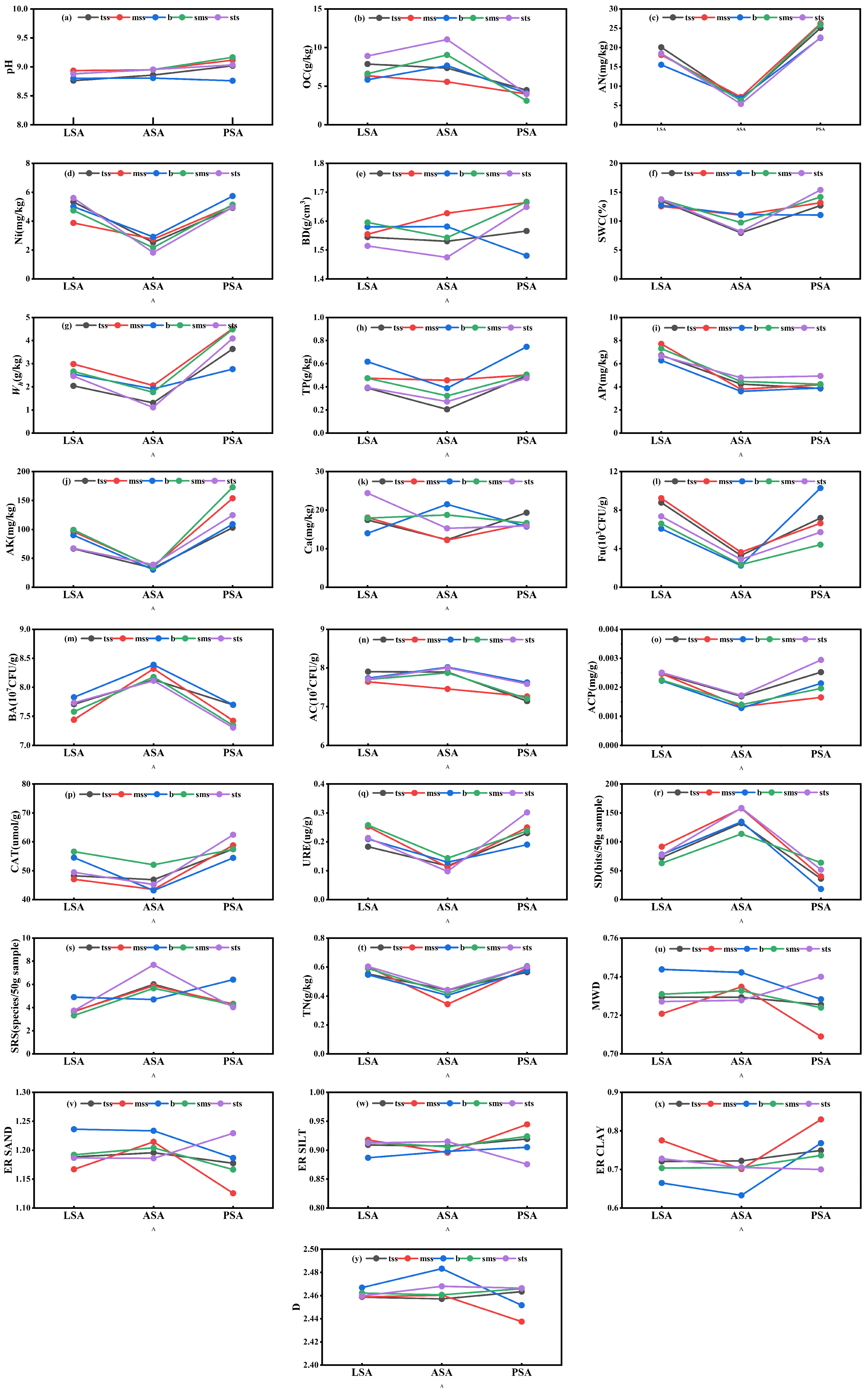
3.1. Ecological Stoichiometric Among Soil Samples

In the study area, we selected 23 soil indicators for inclusion in the TDS, which were as follows: pH, OC, TN, AN, Ni, BD, sand, silt, clay, SWC, W_h, TP, AP, AK, Ca, Fu, BA, AC, ACP, CAT, URE, SD, and SRS. As shown in Figure 2, there were also five indicators representing soil texture, MWD, ER_Sand, ER_silt, ER_clay, and D, which were included as well. Among all the factors (Figure 2), AN, Ni, SWC, W_h, TP, AP, AK, Fu, ACP, CAT, URE, TN, and ER_clay exhibited a ‘V-shaped’ variation trend between LSA, ASA, and PSA. The overall levels of PSA and LSA were higher than ASA, with the soil indicator values in LSA, located on the sunny slope, being slightly higher than those in the shady slope, while PSA, located on the shady slope, had slightly higher values than the sunny slope. The distribution differences of pH and BD across different regions were relatively small. The content of OC was lowest in the PSA region. In terms of soil microorganisms, the AC region showed slight distribution differences, while the BA level is slightly higher in the ASA region compared to LSA and PSA, with slight differences.

3.2. Filtration of Soil Dataset

After Welch’s ANOVA test, there was no significant difference between the values of TK, AKP, NP, SC, SWI, and SI in the original soil property index set in different types of regions; therefore, the above indexes were screened out, and the other indexes were used for TDS for SQ evaluation. After PCA analysis of the soil indices comprising TDS, it was found that 72.3% of the variance variation of the soil property indices was explained by the eight groups of principal components.

According to the difference in the distribution of the principal component of a single soil index and the difference in the calculation result of Norm, the soil index of TDS was divided into nine groups, and the soil property index finally selected into MDS was as follows: the first principal component was selected W_h and AN, the second one was selected silt, the third one was selected Ca, the fifth one was selected BD, the sixth one was selected SWC, the seventh one was selected clay, and the ninth one was selected AC. The overall load values of the fourth and the eighth ones were low, and no index was selected (

Table 5. The results of principal component analysis of selected soil property indexes were studied.

Indicators	Principal Component Analysis (PCA)									Norm	Group
	PC1	PC2	PC3	PC4	PC5	PC6	PC7	PC8	PC9
Eigenvalues	3.883	2.562	2.231	1.937	1.508	1.267	1.172	1.067	1.003
Variance contribution/%	16.881	11.139	9.699	8.421	6.555	5.510	5.097	4.639	4.359
Cumulative contribution/%	16.881	28.020	37.719	46.141	52.696	58.206	63.303	67.942	72.301
pH	−0.171	0.303	0.068	0.331	−0.573	0.193	0.165	0.258	−0.088	1.11	5
OC	−0.252	0.029	0.702	0.019	0.058	0.104	−0.115	0.265	0.220	1.23	3
TN	0.665	0.261	0.274	0.129	−0.130	0.031	−0.151	−0.118	0.138	1.48	1
AN	0.714	−0.252	−0.009	−0.275	−0.084	0.201	−0.020	0.110	−0.143	1.54	1
Ni	0.477	−0.407	−0.223	0.042	0.101	−0.145	0.265	−0.187	0.079	1.26	1
BD	0.213	0.014	−0.468	0.010	0.501	0.372	0.116	0.255	−0.194	1.16	5
Sand	0.061	0.639	−0.243	−0.662	−0.091	0.163	−0.057	−0.118	0.136	1.46	4
Silt	−0.028	−0.691	0.166	0.629	0.149	−0.205	−0.061	0.060	−0.043	1.47	2
Clay	−0.140	0.217	0.323	0.140	−0.246	0.179	0.494	0.244	−0.394	1.05	7
SWC	0.363	0.074	−0.017	0.264	0.344	0.398	0.237	−0.114	0.265	1.09	6
Wh	0.742	0.375	0.089	0.140	0.125	−0.031	0.192	0.260	−0.020	1.64	1
TP	0.236	−0.181	−0.361	−0.061	−0.275	−0.319	0.439	0.176	0.361	1.11	7
AP	0.471	−0.382	0.255	−0.271	−0.029	0.265	−0.312	0.136	0.096	1.33	1
AK	0.682	0.319	−0.204	0.255	−0.202	−0.065	−0.111	0.126	0.158	1.55	1
Ca	−0.226	0.085	0.634	−0.201	0.376	0.134	0.200	0.141	0.303	1.26	3
Fu	−0.018	−0.563	−0.109	−0.056	0.024	0.420	0.108	0.096	0.040	1.05	2
BA	−0.640	−0.057	−0.286	0.084	−0.095	0.392	0.122	−0.314	−0.019	1.46	1
AC	−0.362	0.001	0.024	0.280	−0.278	0.276	0.058	−0.195	0.443	1.06	9
ACP	0.199	−0.129	0.024	0.142	−0.271	0.287	−0.399	−0.016	−0.242	0.83	7
CAT	0.162	0.285	0.471	−0.041	0.258	−0.140	0.226	−0.442	−0.306	1.14	3
URE	0.592	0.048	0.294	0.342	−0.165	0.127	0.029	−0.415	0.026	1.43	1
SD	−0.015	0.449	−0.369	0.514	0.309	0.134	−0.125	−0.026	0.003	1.23	4
SRS	−0.329	0.427	−0.105	0.340	0.240	−0.149	−0.288	0.216	0.092	1.19	2

).

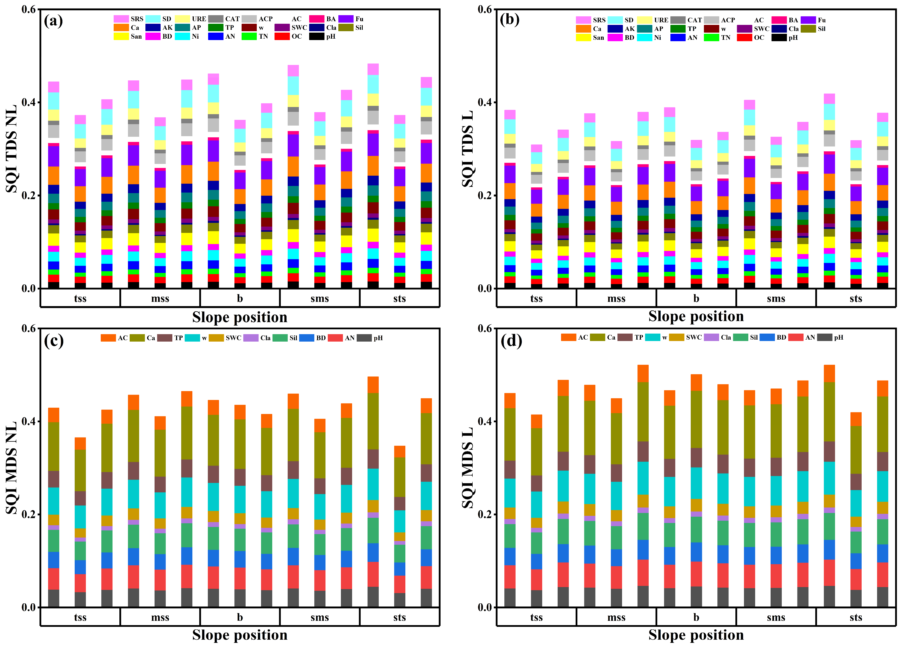
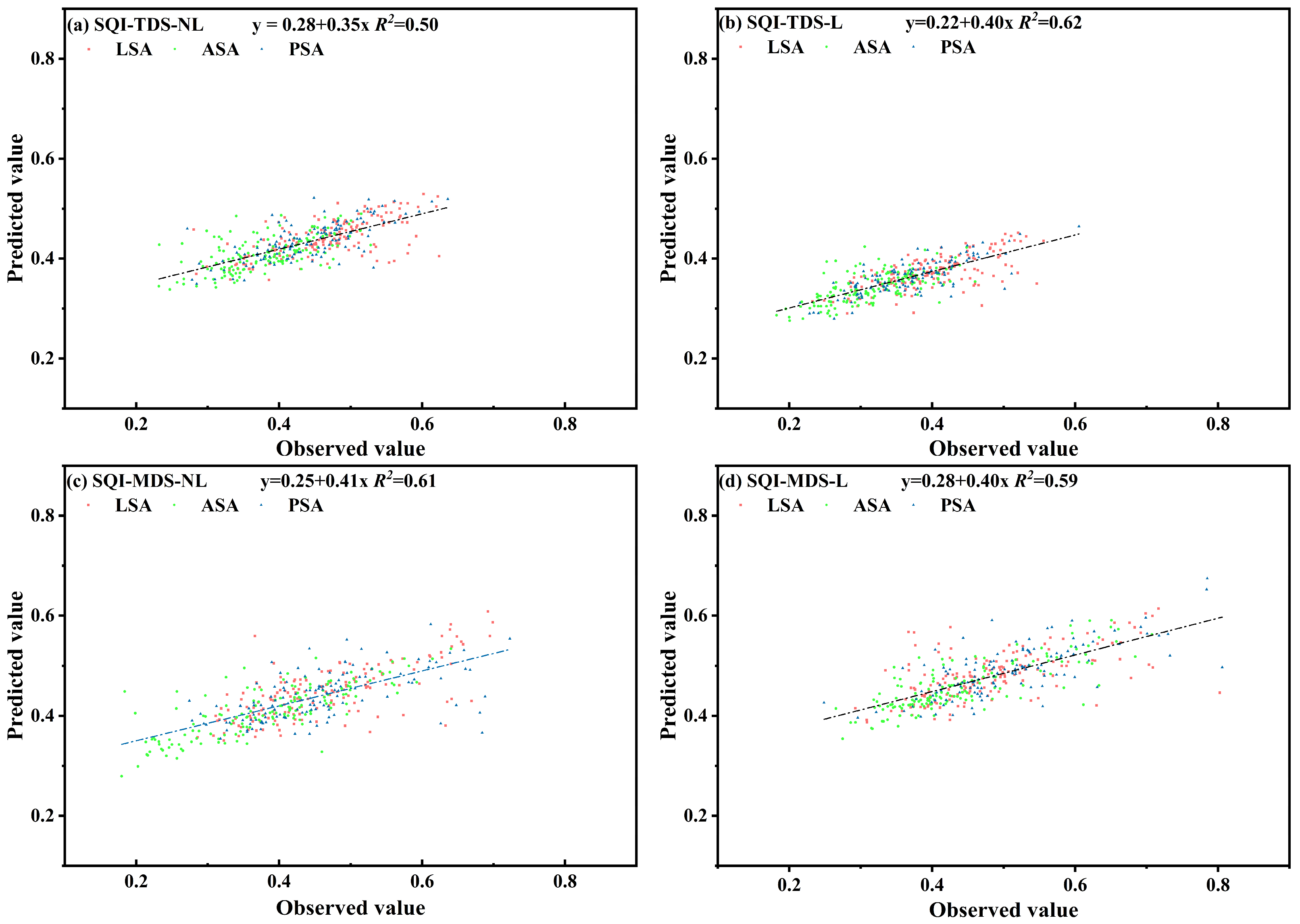
3.3. SQI Discrepancy and Driving Factors

According to the SQI calculation, the score calculated by using a non-linear function was slightly higher than that by using a linear function. MDS and TDS composed of AC, Ca, TP, W_h, SWC, clay, silt, BD, AN, and pH were screened by principal component analysis, and the results were basically consistent at soil sampling points of different slope locations. This indicates that the MDS composition could well reflect the spatial variation of SQI. The SQI value in the ASA was generally lower than that in the LSA and PSA (Figure 3).

From Figure 4, it can be observed that using Random Forest regression produces a good fit for the originally calculated SQI values. The SQI calculated using the linear scoring method based on TDS is slightly smaller (Figure 3), which results in a relatively smaller fitting outcome. Meanwhile, the SQI calculated based on MDS maintains the fitting performance of the SQI calculated using TDS, reflecting the reasonableness of MDS in evaluating the soil quality (SQ) of the study area. The fitting results indicate that using the parameters MWD, ER_sand, ER_silt, ER_clay, and D can reflect the differences in SQ across various slope positions and different types of areas.

The number of decision trees (n_tree) in the Random Forest is determined by the trend of out-of-bag (OOB) error. At the same time, the number of variables used for splitting nodes (mtry) is determined by minimizing the OOB error. The study found that when fitting based on the results of the four types of SQI, the OOB error tends to stabilize and no longer decreases further when n_tree > 80. Additionally, the result corresponding to the smallest OOB error is less than 3. The smallest OOB error occurs when the mtry value is between 1 and 2. Therefore, the study sets n_tree to 100 and mtry to 2. When the model is fitted based on SQI calculated using different scoring methods, the feature variables included in the Random Forest model have a significant impact on the model’s predictive ability. The differences in the impact of feature variables on the model’s predictive ability between different SQIs are generally consistent (

Table 6. Parameter fitting results of Random Forest model with different scoring methods.

SQI Scoring Method		SQI TDS NL	SQI TDS L	SQI MDS NL	SQI MDS L
ntree		100	100	100	100
mtry		2	2	2	2
Increased node purity (IncNodePurity)	MWD	0.19	0.17	0.31	0.33
	ERsand	0.32	0.30	0.61	0.57
	ERsilt	0.37	0.35	0.70	0.59
	ERclay	0.42	0.36	0.76	0.65
	D	0.28	0.27	0.51	0.45
Increased mean squared error (IncMSE)	MWD	6.33	4.19	4.93	4.77
	ERsand	7.15	8.01	7.57	8.07
	ERsilt	5.07	4.80	7.86	8.31
	ERclay	4.87	5.41	5.79	5.12
	D	3.48	0.61	5.85	4.21
Fitting effect on training data	RMSE	0.04	0.04	0.06	0.06
	R2	0.77	0.76	0.76	0.78
	MAE	0.04	0.03	0.05	0.04
Fitting effect on testing data	RMSE	0.09	0.007	0.012	0.011
	R2	2 × 10−3	5.4 × 10−8	9 × 10−5	1 × 10−3
	MAE	0.07	0.06	0.09	0.09

). Among them, the ER feature variables have the most significant impact on the model’s predictive performance, followed by D, with MWD having a relatively weaker effect.

4. Discussion

4.1. Soil Indicators and Environmental Factors

In the Pisha Sandstone areas, soil plays a crucial role as it serves as a medium for microbial activity and vegetation survival. It also retains moisture and facilitates nutrient cycling. A healthy soil environment provides favorable conditions for vegetation growth, regional land productivity, and human activities [43,44]. To objectively and accurately assess soil conditions, the study selected physical, chemical, and biological indicators to evaluate the soil’s status, offering a theoretical basis for ecological construction in the study regions. The uniqueness of the study area lay in the distinctive lithology of the sandstone, where the soil layer is relatively thin. The surface soil, consisting of sand, becomes muddy upon contact with water and is easily eroded during rainfall. Apart from soil pH and bulk density, significant differences in soil composition were observed across different study areas. The general trend is as follows: LSA > PSA > ASA, with ASA showing significantly lower content compared to LSA and PSA. Soil indicators such as total nitrogen (TN), ammonium nitrogen (AN), nitrate nitrogen (Ni), soil water content (SWC), water holding capacity (W_h), total phosphorus (TP), available phosphorus (AP), and available potassium (AK) were generally slightly higher in PSA compared to LSA and significantly higher than in ASA. The causes of these differences may be attributed to variations in soil texture, human activities, and different levels of erosion impacts [45,46,47]. The results indicated that the sand enrichment rate in PSA soil particles was lower than that in LSA and ASA, while the enrichment rates of silt and clay were relatively higher, particularly in the middle of the slope and at the bottom of the ditch. This suggests that, compared to PSA, the finer soil particles in LSA and ASA were more prone to erosion, leaving behind only coarse particles at the original slope positions. This was unfavorable for maintaining soil quality. Due to the substantial influence of human activities, soil quality in the LSA was found to be superior. This trend was more commonly observed in the study areas.

Soil enzyme activity is closely associated with soil microorganisms and nutrient content, serving as a direct reflection of microbial activity and soil functions [48,49]. Research has shown that the content of soil sucrase (SC) is closely related to the organic carbon (OC) content, while the activity of soil urease is closely linked to the total nitrogen (TN) content. These findings were consistent with the studies of Cheng [50] and Song [51]. Significant differences in soil enzyme activity, microbial activity, and nutrient content were observed across different study areas. Urease is released through soil microbial metabolism, and after urease hydrolyzes urea, it forms a substantial amount of carbonate ions. The mineral composition of sandstone contains a significant amount of montmorillonite [52], which gives the sandstone particles strong ion exchange and adsorption capabilities. The calcium ions within the sandstone readily combine with the carbonate ions, resulting in the deposition and release of calcium carbonate. The deposition of calcium carbonate altered the mechanical properties of the soil particles, promoting the aggregation and cementation of sandstone particles to some extent. Research indicated that Pisha sandstone particles could effectively block the rapid infiltration of sandy soil, suggesting that the porosity of the sandstone particles is improved [53]. The planting of Hippophae rhamnoides in the study region, especially LSA and PSA, has helped retain atmospheric nitrogen as a soil nutrient within the sandstone particles, thus improving soil nutrient conditions. Soil urease activity could be stimulated, creating a positive cycle, which aligns with the findings of Fu [54].

4.2. Soil Quality Assessment Methods and Differences

Quantitative assessment of soil quality is a vital component of ecological and environmental evaluation. Due to its convenient experimental processes and the clear, visual results it provides, the application of soil quality assessment is widespread [55]. Therefore, it was crucial to select appropriate soil indicators and incorporate them into the overall dataset when determining the soil quality index. The total dataset of soil indicators should accurately assess soil quality levels and be sensitive to changes in the soil quality index. To avoid redundancy caused by an excess of soil indicator values, using a minimal dataset to replace the full dataset—while still preserving the effectiveness of the indicator information—could help reduce both time and material costs, highlighting the key indicators that most significantly influence soil quality levels [9,56,57].

The non-linear (NL) and linear (L) scoring methods used in this study to calculate the soil quality index (SQI) were both standardized approaches, which allowed the selected soil indicators to reflect the actual state of soil quality (SQ) as accurately as possible [58,59]. To identify the most suitable method for evaluating soil quality, the study employed both NL and L scoring methods simultaneously, ensuring that the SQ results were represented by dimensionless values between 0 and 1. The differences in SQI values highlighted variations in SQ and the applicability of the two scoring methods. According to the results, the MDS (minimal dataset) generated by the PCA (principal component analysis) dimensionality reduction method significantly reduced information redundancy while preserving essential SQ data [57]. The study found no significant differences in the SQI calculated using the TDS (total dataset) and MDS indicator sets based on the S_NL (non-linear scoring) method (R² = 0.96) and the S_L (linear scoring) method (R² = 0.96). This suggests that the current MDS dataset could be effectively used to assess soil quality levels in the study areas. Indicators related to soil texture, such as bulk density (BD), silt, and clay, can influence the survival and community structure of soil microorganisms, significantly impacting soil fertility and vegetation community structure [60]. Soil ammonium nitrogen (AN) can attach to soil colloids in the form of fine textures, which helps retain AN in fine soil particles. Similar to AN, the activity of soil microorganisms can release organic phosphorus (organic P), and soluble phosphorus (soluble P) is easily adsorbed by fine soil particles, which are then absorbed by plant roots. Phosphorus (P) is particularly scarce in the study area, and total phosphorus (TP) and available phosphorus (AP) in the soil can effectively indicate microbial activity and soil quality while also demonstrating how the effectiveness of total nitrogen (TN) and TP can impact soil quality and its ecological functions [61]. Additionally, soil moisture content plays a critical role in influencing both soil quality and microbial activity.

5. Conclusions

In this study, principal component analysis (PCA), the entropy weight method, and the Random Forest (RF) model were applied to evaluate and predict soil quality index (SQI) through double datasets (TDS and MDS) and double scoring function methods (S_NL and S_L) among LSA, ASA, and PSA. The results revealed that indicators such as pH, ammonia nitrogen (AN), bulk density (BD), silt content (silt), clay content (clay), soil water content (SWC), hygroscopic water content (W_h), total phosphorus (TP), soluble calcium (Ca), and actinomycetes (Ac) were reliable for representing the soil quality index (SQI). Among the methods tested, the non-linear scoring method showed better applicability for soil quality evaluation. Compared to MWD, parameters D and ER were more effective in capturing the differences and distribution of soil quality in the Pisha sandstone area. The soil quality results indicated that the SQI values predicted by the RF model closely matched those obtained through PCA, suggesting that slope erosion tests and the soil wet sieving method are both effective for predicting and assessing soil quality in the Pisha sandstone region. In areas dominated by coarse sand particles, the surface soil has suffered from severe slope erosion over an extended period. The unique soil structure in these areas leads to poor soil quality levels. Consequently, the ecological management measures of the soil are a critical factor to consider in maintaining soil quality and health in the Pisha sandstone area.

References

1. Bone, J.; Head, M.; Barraclough, D.; Archer, M.; Scheib, C.; Flight, D.; Voulvoulis, N. Soil quality assessment under emerging regulatory requirements. Environ. Int. 2010, 36, 609–622. [Google Scholar] [CrossRef] [PubMed]
2. Koch, A.; Chappell, A.; Eyres, M.; Scott, E. Monitor Soil Degradation or Triage for Soil Security? An Australian Challenge. Sustainability 2015, 7, 4870–4892. [Google Scholar] [CrossRef]
3. Lee, J.; Park, C.; Rhee, H. Revegetation of decomposed granite roadcuts in Korea: Developing digger, evaluating cost effectiveness, and determining dimensions of drilling holes, revegetation species, and mulching treatment. Land Degrad. Dev. 2013, 24, 591–604. [Google Scholar] [CrossRef]
4. He, L.; Guo, J.; Zhang, X.; Liu, B.; Guzman, G.; Gomeza, J. Vegetation restoration dominated the attenuated soil loss rate on the Loess Plateau, China over the last 50 years. CATENA 2023, 228, 107149. [Google Scholar] [CrossRef]
5. Anley, M.A.; Minale, A.S. Modeling the impact of land use land cover change on the estimation of soil loss and sediment export using Invest model at the Rib watershed of Upper Blue Nile Basin, Ethiopia. Remote Sens. Appl. 2024, 34, 101177. [Google Scholar] [CrossRef]
6. Schoenholtz, S.; Miegroet, H.; Burger, J. A review of chemical and physical properties as indicators of forest soil quality: Challenges and opportunities. Forest Ecol. Manag. 2000, 138, 335–356. [Google Scholar] [CrossRef]
7. Bünemann, E.; Bongiorno, G.; Bai, Z.G.; Creamer, R.E.; De Deyn, G.; de Goede, R.; Fleskens, L.; Geissen, V.; Kuyper, T.W.; Mäder, P.; et al. Soil quality: A critical review. Soil Biol. Biochem. 2018, 120, 105–125. [Google Scholar] [CrossRef]
8. Yu, P.; Liu, J.; Tang, H.; Sun, X.; Liu, S.; Tang, X.; Ding, Z.; Ma, M.; Ci, E. Establishing a soil quality index to evaluate soil quality after afforestation in a karst region of Southwest China. CATENA 2023, 230, 107237. [Google Scholar] [CrossRef]
9. Raiesi, F.; Kabiri, V. Identification of soil quality indicators for assessing the effect of different tillage practices through a soil quality index in a semi-arid environment. Ecol. Indic. 2016, 71, 198–207. [Google Scholar] [CrossRef]
10. Huang, W.; Zong, M.; Fan, Z.; Feng, Y.; Li, S.; Duan, C.; Li, H. Determining the impacts of deforestation and corn cultivation on soil quality in tropical acidic red soils using a soil quality index. Ecol. Indic. 2021, 125, 52–61. [Google Scholar] [CrossRef]
11. Zahedifar, M. Assessing alteration of soil quality, degradation, and resistance indices under different land uses through network and factor analysis. CATENA 2023, 222, 106807. [Google Scholar] [CrossRef]
12. Zhu, N.; Yan, Y.; Bai, K.; Zhang, J.; Wang, C.; Wang, X.; Xu, D.; Liu, J.; Xin, X.; Chen, J. Conversion of croplands to shrublands does not improve soil organic carbon and nitrogen but reduces soil phosphorus in a temperate grassland of northern China. Geoderma 2023, 432, 116407. [Google Scholar] [CrossRef]
13. Dong, L.B.; Li, J.W.; Zhang, Y.; Bing, M.Y.; Liu, Y.L.; Wu, J.Z.; Hai, X.Y.; Li, A.; Wang, K.B.; Wu, P.X.; et al. Effects of vegetation restoration types on soil nutrients and soil erodibility regulated by slope positions on the Loess Plateau. J. Environ. Manag. 2022, 302, 113985. [Google Scholar] [CrossRef]
14. Karaca, S.; Dengiz, O.; Demira, Ğ.; Turan, İ.; Özkan, B.; Dedeoglu, M.; Gülser, F.; Sargin, B.; Demirkaya, S.; Ay, A. An assessment of pasture soils quality based on multi-indicator weighting approaches in semi-arid ecosystem. Ecol. Indic. 2021, 121, 107001. [Google Scholar] [CrossRef]
15. Nortcliff, S. Standardization of soil quality attributes. Agr. Ecosyst. Environ. 2002, 88, 161–168. [Google Scholar] [CrossRef]
16. Askari, M.S.; Holden, N.M. Indices for quantitative evaluation of soil quality under grassland management. Geoderma 2014, 230, 131–142. [Google Scholar] [CrossRef]
17. Yao, W.; Xiao, P. Ecological Comprehensive Management Theory and Technology of Pisha Sandstone Area; Science Press: Beijing, China, 2021; Chapters 1–2. [Google Scholar]
18. Wang, R.; Yan, F.; Wang, Y. Vegetation Growth Status and Topographic Effects in the Pisha Sandstone Area of China. Remote Sens. 2020, 12, 2759. [Google Scholar] [CrossRef]
19. Ren, X.; Chai, X.; Qu, Y.; Xu, Y.; Khan, F.; Wang, J.; Geming, P.; Wang, W.; Zhang, Q.; Wu, Q.; et al. Restoration of Grassland Improves Soil Infiltration Capacity in Water-Wind Erosion Crisscross Region of China’s Loess Plateau. Land 2023, 12, 1485. [Google Scholar] [CrossRef]
20. Zhu, R.; Yu, Y.; Zhao, J.; Liu, D.; Cai, S.; Feng, J.; Rodrigo-Comino, J. Evaluating the applicability of the water erosion prediction project (WEPP) model to runoff and soil loss of sandstone reliefs in the Loess Plateau, China. Int. Soil Water Conserv. 2023, 11, 240–250. [Google Scholar] [CrossRef]
21. Tian, X.; Tian, P.; Zhao, G.; Gómez, J.A.; Guo, J.; Mu, X.; Gao, P.; Sun, W. Sediment source tracing during flood events in the Huangfu River basin in the northern Loess Plateau, China. J. Hydrol. 2023, 620, 129540. [Google Scholar] [CrossRef]
22. Fan, S.; Qin, F.; Che, Z. Geochemical indicators to constrain weathering, provenance and tectonic setting of the Pisha Sandstone (Early-Middle Triassic) in Northeast Ordos Basin, China. Heliyon 2024, 10, e29120. [Google Scholar] [CrossRef] [PubMed]
23. Jing, Y.; Liu, X.; Qiao, Z.; Liu, Z.; Pang, Y.; Qi, H.; Wang, J. Mixture-proportioning design of cement soil containing Pisha sandstone for mine filling. Case Stud. Constr. Mat. 2024, 20, e02904. [Google Scholar] [CrossRef]
24. Ma, W.; Yang, K.; Zhou, X.; Luo, Z.; Guo, Y. Effect of Hydrophilic Polyurethane on Interfacial Shear Strength of Pisha Sandstone Consolidation under Freeze-Thaw Cycles. Polymers 2023, 15, 2131. [Google Scholar] [CrossRef] [PubMed]
25. Zhou, L.; Li, J.; Xu, C.; Du, W.; Liu, Z.; Hu, F. Effects of Pisha sandstone additions on microstructural stability of sandy soil in Mu Us Sandy Land, China. Soil Till. Res. 2025, 248, 106437. [Google Scholar] [CrossRef]
26. Feng, Z.; Li, X. Microbially induced calcite precipitation and synergistic mineralization cementation mechanism of Pisha sandstone components. Sci. Total Environ. 2023, 866, 161348. [Google Scholar] [CrossRef]
27. Shahid, S.A. United Arab Emirates Keys to Soil Taxonomy; Springer: Dordrecht, The Netherlands, 2014. [Google Scholar]
28. Yu, P.J.; Liu, S.W.; Zhang, L.; Li, Q.; Zhou, D.W. Selecting the minimum data set and quantitative soil quality indexing of alkaline soils under different land uses in northeastern China. Sci. Total Environ. 2018, 616–617, 564–571. [Google Scholar] [CrossRef]
29. Mamehpour, N.; Rezapour, S.; Ghaemian, N. Quantitative assessment of soil quality indices for urban croplands in a calcareous semi-arid ecosystem. Geoderma 2021, 382, 114781. [Google Scholar] [CrossRef]
30. Liu, G. Soil Physical and Chemical Analysis & Description of Soil Profiles; Standards Press of China: Beijing, China, 1996. [Google Scholar]
31. Lu, R.K. Analysis Methods of Soil Agricultural Chemistry; China Agricultural Science and Technology Press: Beijing, China, 1999. [Google Scholar]
32. Elsas, J.D.V. Methods of soil analysis. Part 2—Microbiological and biochemical properties. Sci. Hortic. 1995, 63, 131–133. [Google Scholar] [CrossRef]
33. Gerdemann, J.W.; Nicolson, T.H.; Gerdemann, J.W.; Nicolson, T.H. Spores of mycorrhizal Endogone extracted from soil by wet sieving and decanting. Trans. Brit. Mycol. Soc. 1963, 46, 235–244. [Google Scholar] [CrossRef]
34. Andrew, S.S.; Karlen, D.L.; Cambardella, C.A. The Soil Management Assessment Framework: A Quantitative Soil Quality Evaluation Method. Soil Sci. Soc. Am. J. 2004, 68, 1945–1962. [Google Scholar] [CrossRef]
35. Cherubin, M.R.; Tormena, C.A.; Karlen, D.L. Soil quality evaluation using the soil management assessment framework (SMAF) in Brazilian Oxi-sols with contrasting texture. Rev. Bras. Cienc. Solo 2017, 41, e0160148. [Google Scholar] [CrossRef]
36. Mukherjee, A.; Lal, R. The biochar dilemma. Soil Res. 2014, 52, 217–230. [Google Scholar] [CrossRef]
37. Chen, Y.D.; Wang, H.Y.; Zhou, J.M.; Xing, L.; Zhu, B.S.; Zhao, Y.C.; Chen, X.Q. Minimum Data Set for Assessing Soil Quality in Farmland of Northeast China. Pedosphere 2013, 23, 564–576. [Google Scholar] [CrossRef]
38. Gan, F.; Shi, H.; Yan, Y.; Pu, J.; Dai, Q.; Gou, J.; Fan, Y. Soil quality assessment of karst trough valley under different bedrock strata dip and land-use types, based on a minimum data set. CATENA 2024, 241, 108048. [Google Scholar] [CrossRef]
39. Ma, J.; Chen, Y.; Zhou, J.; Wang, K.B.; Wu, J. Soil quality should be accurate evaluated at the beginning of lifecycle after land consolidation for eco-sustainable development on the Loess Plateau. J. Clean. Prod. 2020, 267, 122244. [Google Scholar] [CrossRef]
40. Heung, B.; Bulmer, C.E.; Schmidt, M.G. Predictive soil parent material mapping at a regional-scale: A Random Forest approach. Geoderma 2014, 214–215, 141–154. [Google Scholar] [CrossRef]
41. Taghizadeh-Mehrjardi, R.; Nabiollahi, K.; Kerry, R. Digital mapping of soil organic carbon at multiple depths using different data mining techniques in Baneh region, Iran. Geoderma 2016, 266, 98–110. [Google Scholar] [CrossRef]
42. Taghizadeh-Mehrjardi, R.; Schmidt, K.; Amirian-Chakan, A.; Rentschler, T.; Zeraatpisheh, M.; Sarmadian, F.; Valavi, R.; Davatgar, N.; Behrens, T.; Scholten, T. Improving the Spatial Prediction of Soil Organic Carbon Content in Two Contrasting Climatic Regions by Stacking Machine Learning Models and Rescanning Covariate Space. Remote Sens. 2020, 12, 1095. [Google Scholar] [CrossRef]
43. Liu, J.; Vu, N.H.; Zhen, S.; Zhu, H.; Fei, Z.; Zhong, Z. Characteristics of bulk and rhizosphere soil microbial community in an ancient Platycladus orientalis forest. Appl. Soil Ecol. 2018, 132, 91–98. [Google Scholar] [CrossRef]
44. Getahun, G.T.; Ktterer, T.; Munkholm, L.J.; Parvage, M.M.; Kirchmann, H. Short-term effects of loosening and incorporation of straw slurry into the upper subsoil on soil physical properties and crop yield. Soil Till. Res. 2018, 184, 62–67. [Google Scholar] [CrossRef]
45. Negis, H.; Eker, C.S.; Erci, V.; Gumus, I. Establishment of a minimum dataset and soil quality assessment for multiple reclaimed areas on a wind-eroded region. CATENA 2023, 229, 107208. [Google Scholar] [CrossRef]
46. Li, W.; Liu, Y.; Zheng, H.; Wu, J.; Yuan, H.; Wang, X.; Xie, W.; Qin, Y.; Zhu, H.; Nie, X.; et al. Complex vegetation patterns improve soil nutrients and maintain stoichiometric balance of terrace wall aggregates over long periods of vegetation recovery. CATENA 2023, 227, 107141. [Google Scholar] [CrossRef]
47. Wang, H.; Yang, J.; Finn, D.R.; Brunotte, J.; Tebbe, C.C. Distinct seasonal and annual variability of prokaryotes, fungi and protists in cropland soil under different tillage systems and soil texture. Soil Biol. Biochem. 2025, 203, 109732. [Google Scholar] [CrossRef]
48. Adetunji, A.T.; Lewu, F.B.; Mulidzi, R.; Ncube, B. The biological activities of 2-glucosidase, phosphatase and urease as soil quality indicators: A review. J. Soil Sci. Plant Nut. 2017, 17, 794–807. [Google Scholar] [CrossRef]
49. de Andrade Barbosa, M.; de Sousa Ferraz, R.L.; Coutinho, E.L.M.; Coutinho Neto, A.M.; da Silva, M.S.; Fernandes, C.; Rigobelo, E.C. Multivariate analysis and modeling of soil quality indicators in long-term management systems. Sci. Total Environ. 2019, 657, 457–465. [Google Scholar] [CrossRef]
50. Cheng, C.; Gao, M.; Zhang, Y.; Long, M.; Wu, Y.; Li, X. Effects of disturbance to moss biocrusts on soil nutrients, enzyme activities, and microbial communities in degraded karst landscapes in southwest China. Soil Biol. Biochem. 2021, 152, 108065. [Google Scholar] [CrossRef]
51. Song, X.; Yang, J.; Hussain, Q.; Liu, X.; Zhang, J.; Cui, D. Stable isotopes reveal the formation diversity of humic substances derived from different cotton straw-based materials. Sci. Total Environ. 2020, 740, 140202. [Google Scholar] [CrossRef]
52. Fan, Y.X.; Lu, S.X.; He, M.; Yang, L.M.; Hu, M.F.; Yang, Z.J.; Liu, X.F.; Hui, D.F.; Guo, J.F.; Yang, Y.S. Long-term throughfall exclusion decreases soil organic phosphorus associated with reduced plant roots and soil microbial biomass in a subtropical forest. Geoderma 2021, 404, 115309. [Google Scholar] [CrossRef]
53. Wang, L.; Liu, S. Mechanism of sand cementation with an efficient method of microbial-induced calcite precipitation. Materials 2021, 14, 5631. [Google Scholar] [CrossRef]
54. Fu, B.; Qi, Y.B.; Chang, Q.R. Impacts of revegetation management modes on soil properties and vegetation ecological restoration in degraded sandy grassland in farming-pastoral ecotone. Int. J. Agric. Biol. Eng. 2015, 8, 26–34. [Google Scholar]
55. Doran, J.W.; Parkin, T.B. Defining and Assessing Soil Quality; John Wiley & Sons, Inc.: Hoboken, NJ, USA, 2015. [Google Scholar]
56. Zhou, Y.; Ma, H.; Xie, Y.; Jia, X.; Su, T.; Li, J.; Shen, Y. Assessment of soil quality indexes for different land use types in typical steppe in the loess hilly area, China. Ecol. Indic. 2020, 118, 106743. [Google Scholar] [CrossRef]
57. Iheshiulo, E.M.A.; Larney, F.J.; Hernandez-Ramirez, G.; St. Luce, M.; Chau, H.W.; Liu, K. Quantitative evaluation of soil health based on a minimum dataset under various short-term crop rotations on the Canadian prairies. Sci. Total Environ. 2024, 935, 173335. [Google Scholar] [CrossRef] [PubMed]
58. Mahajan, G.; Das, B.; Morajkar, S.; Desai, A.; Murgaokar, D.; Kulkarni, R.; Sale, R.; Patel, K. Soil quality assessment of coastal salt-affected acid soils of India. Environ. Sci. Pollut. Res. 2020, 27, 26221–26238. [Google Scholar] [CrossRef]
59. Nabiollahi, K.; Golmohamadi, F.; Taghizadeh-Mehrjardi, R.; Kerry, R.; Davari, M. Assessing the effects of slope gradient and land use change on soil quality degradation through digital mapping of soil quality indices and soil loss rate. Geoderma 2018, 318, 16–28. [Google Scholar] [CrossRef]
60. Moebius, B.N.; van Es, H.M.; Schindelbeck, R.R.; Idowu, O.J.; Clune, D.J.; Thies, J.E. Evaluation of laboratory-measured soil properties as indicators of soil physical quality. Soil Sci. 2007, 172, 895–912. [Google Scholar] [CrossRef]
61. Liu, W.F.; Huang, Z.; Guo, Z.; Lopez-Vicente, M.; Wang, Z.; Wu, G.L. A nature-based solution to reduce soil water vertical leakage in arid sandy land. Geoderma 2023, 438, 116630. [Google Scholar] [CrossRef]
Figure 1. Location of the study region and sample sites.
Forests 16 00699 g001
Figure 2. Concentrations of soil indicators in different types of regions in the study: Loess soil area (LSA), aeolian soil area (ASA), typical Pisha sandstone area (PSA). Different slope positions in figures: sunny top slope (tss), sunny middle slope (mss), bottom (b), shady middle slope (sms), shady top slope (sts). (a) pH, (b) organic carbon (OC), (c) ammonia nitrogen (AN), (d) nitrate (Ni), (e) bulk density (BD), (f) soil water content (SWC), (g) hydroscopic water content (Wh), (h) total phosphorus (TP), (i) available phosphorus (AP), (j) available potassium (AK), (k) soluble calcium (Ca), (l) culturable fungi (Fu), (m) culturable bacteria (BA), (n) culturable actinomycetes (AC), (o) acid phosphatase (ACP), (p) activity of catalase (CAT), (q) activity of urease (URE), (r) spore density (SD), (s) spore richness (SRS), (t) total nitrogen (TN), (u) mean weight diameter (MWD), (v) enrichment rate of sand (ERsand), (w) enrichment rate of silt (ERsilt), (x) enrichment rate of clay (ERclay), (y) fractal dimension (D).
Forests 16 00699 g002
Figure 3. Soil quality index with total datasets and minimum datasets under non-linear and linear scoring methods and weight distribution at each slope position. (a) Soil quality index with total datasets under non-linear scoring method (SQI TDS NL), (b) soil quality index with total datasets under linear scoring method (SQI TDS L), (c) soil quality index with minimum datasets under non-linear scoring method (SQI MDS NL), (d) soil quality index with minimum datasets under linear scoring method (SQI MDS L). Different slope positions in figures: tss: sunny top slope; mss: sunny middle slope; b: bottom of the trench; sms: shady middle slope; sts: shady top slope.
Forests 16 00699 g003
Figure 4. Random Forest model regression prediction in different soil quality indexes resulted from mean weight diameter (MWD), enrichment rate of sand (ERsand), enrichment rate of silt (ERsilt), enrichment rate of clay (ERclay), and fractal dimension (D). (a) Soil quality index with total datasets under non-linear scoring method (SQI TDS NL), (b) soil quality index with total datasets under linear scoring method (SQI TDS L), (c) soil quality index with minimum datasets under non-linear scoring method (SQI MDS NL), (d) soil quality index with minimum datasets under linear scoring method (SQI MDS L). Loess soil area (LSA), aeolian soil area (ASA), Pisha sandstone area (PSA).
Forests 16 00699 g004