Article

Effects of Topographic and Soil Factors on Woody Species Assembly in a Chinese Subtropical Evergreen Broadleaved Forest

1
Faculty of Life Science and Technology, Central South University of Forestry and Technology, Changsha 410004, Hunan, China
2
Faculty of Forestry, Central South University of Forestry and Technology, Changsha 410004, Hunan, China
3
Institute of Environment Sciences, Department of Biological Sciences, University of Quebec at Montreal, Montreal, QC H3C-3P8, Canada
*
Author to whom correspondence should be addressed.
Forests 2015, 6(3), 650-669; https://doi.org/10.3390/f6030650
Submission received: 5 December 2014 / Revised: 15 February 2015 / Accepted: 28 February 2015 / Published: 6 March 2015

Abstract

:
Evergreen broadleaved forests in subtropical China contain a complicated structure of diverse species. The impact of topographic and soil factors on the assembly of woody species in the forest has been poorly understood. We used Ripley’s K(t) function to analyze the spatial patterns and associations of dominant species and residual analysis (RDA) to quantify the contribution of topography and soil to species assembly. The 1 ha plot investigated had 4797 stems with a diameter at breast height (dbh) larger than 1 cm that belong to 73 species, 55 genera, and 38 families. All stems of the entire forest and four late successional species exhibited a reversed J shape for dbh distribution, while two early successional species showed a unimodal shape. Aggregation was the major spatial pattern for entire forests and dominant species across vertical layers. Spatial associations between inter- and intra-species were mostly independent. Topographic and soil factors explained 28.1% of species assembly. The forest was close to late succession and showed the characteristics of diverse woody species, high regeneration capacity, and aggregated spatial patterns. Topographic and soil factors affected species assembly, but together they could only explain a small part of total variance.

1. Introduction

Floristic composition, structure, and spatial patterns are the fundamental characteristics that reflect species assembly in forests. Species assembly in a forest result from stand development processes [1,2] that are driven by immigration through various means of propagule dispersal [3] and extinction; these are due to species response to environmental conditions [4] and biotic interactions, such as competition, herbivores, and predation [5]. Understanding the underlying processes of species assembly in a forest could provide useful information for predicting stand dynamics and for forest management and biodiversity conservation. In general, two approaches may be followed to analyze the processes that affect species assembly. One is a dynamic approach where the factors affecting changes in species richness are investigated using data collected from the forests at different successional stages [1]. Another is a statistical approach where the factors are inferred from the existing stand structure and spatial pattern using the data collected in a plot [6]. For example, spatial patterns (aggregation, random, and regular) are usually used to interpret species assembly and coexistence [7,8]. It is assumed that aggregation spatial patterns are a common phenomenon for conspecific trees in order to reduce competitive exclusion and promote a more diverse coexistence of species [9]. Many factors, including functional traits (e.g., growth form, shade tolerance, and dispersal modes), life history strategy [10], regeneration strategy [11], disturbances [12], and habitat heterogeneity [13], lead to aggregated distribution.
Some evidence has indicated that habitat heterogeneity plays an important role in regulating the distribution of species [14]. Previous studies reported that species distribution was correlated with variations in topography or soil in tropical [15], subtropical [16,17,18], and temperate forests [19]. However, habitat associations of the majority of species were inconsistent with life stages or vertical layers in tropical and temperate forests [20,21]. Topography and soil variables significantly affected species assembly in China’s subtropics [16,17], but their relative contribution to entire stands and dominant species among vertical layers is poorly understood.
Evergreen broadleaved forests in subtropical areas of China are climax vegetation with diverse species, high stability, and productivity [22]. The favorable climate results in diverse evergreen broadleaved forests [12]. However, primary evergreen broadleaved forests had almost disappeared until now and their total area was less than 5% of the original area as a result of clearance for plantations and the conversion into secondary vegetation, due to sustained human disturbance and a timber-centric forestry policy over past decades [23]. Recently, China has changed its forestry policy from timber production to ecosystem services [24]. Close-to-nature forest management occurred just as a practical approach to over exploitation and degradation in fragile mountain landscapes. The general aim of close-to-nature management was to formulate diversely structured and uneven-aged forests on a finer scale [25]. For Chinese subtropical areas, remnants of those surviving original evergreen broadleaved forests are considered as templates of sustainable management for natural forest development. Although numerous studies related to species diversity and coexistence have been conducted in old-growth forests at remote mountain locations [26,27], information remains limited on floristic composition, stand structure, and spatial pattern, as well as on the driving mechanisms of species assembly in subtropical areas of China.
In this study, floristic composition, structure, and spatial patterns were examined to infer the driving processes and to determine the relative contribution of topographic and soil variables to species assembly in an evergreen broadleaved forest primarily dominated by Lithocarpus glaber (Thunb.) Nakai and Cyclobalanopsis glauca (Thunb.) Oerst. The specific objectives of this study were to investigate: (1) characteristics of species composition, and the horizontal and vertical structure of subtropical broadleaved forest; (2) spatial distribution patterns and associations of intraspecific and interspecific species; and (3) how topographic and soil variables affect species abundance and spatial distributions.

2. Materials and Methods

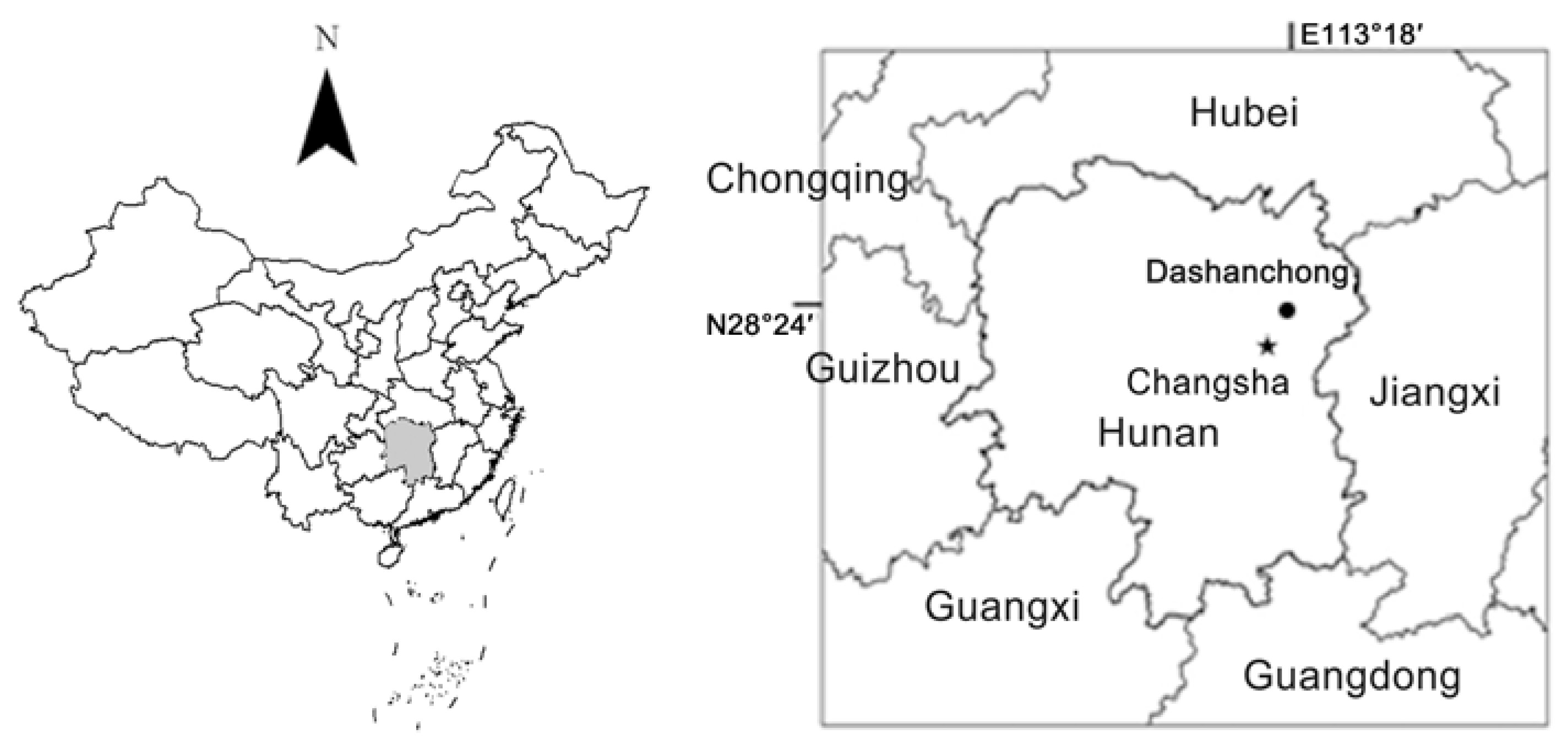
2.1. Site Description

The study site was located at the Dashanchong Forest Farm (28°23′58″–28°24′58″ N, 113°17′46″–113°19′8″ E), Changsha County, Hunan Province, China (Figure 1). This region is typical of a low hilly landscape with an altitude ranging from 55 to 217.4 m above sea level. It lies within a humid mid-subtropical monsoon climate. Annual mean air temperature ranges from 16.6 to 17.6 °C, with a mean monthly minimum temperature of −11 °C in January and maximum temperature of 40 °C in July. Mean annual precipitation is 1412–1559 mm, occurring mostly between April and August. Soil type is designated as well-drained clay loam red soil developed on slate and shale rock, classified as Alliti-Udic Ferrosols. Most forest types are secondary forests at different successional stages following anthropogenic disturbances, such as plantations. Firewood collection has been prohibited since the late 1970s. L. glaber-C. glauca forest is the common well-preserved evergreen broadleaved forest in the area [28].
Figure 1. Location of the 1 ha permanent plot of subtropical broadleaved evergreen forest at Dashanchong Forest Farm, Changsha County, Hunan Province, China.
Forests 06 00650 g001

2.2. Plot Installation and Investigation

A permanent 1 ha plot (100 m × 100 m horizontal distance) was established in 2009. The plot was divided into one hundred 10 m × 10 m subplots for the conduction of a census. All stems larger than 1 cm in diameter at breast height (1.3 m; dbh) were tagged and then accurately mapped to 0.1 m to establish the horizontal position and species identification. Stems originating from the same base were mapped individually when the main stem bifurcated below 1.3 m. Stems whose roots were outside the plot but whose crowns were within the plot boundary were recorded to reduce potential bias introduced by edge effects [29]. For each stem, coordinates (X and Y), dbh, total height (H), height between the lowest live branch and the ground surface (Hl), and two direction crown diameter (Cw) were measured [23].

2.3. Topographic and Soil Data Collection

For each 10 m × 10 m subplot, four topographic variables (mean altitude, slope, convexity, and aspect) were calculated. Mean altitude (m) was the average value of altitudes of the four corners of each subplot. Slope (°) was the mean angular deviation from the horizon of each of the four triangular planes determined by connecting three of its corners [14]. Convexity was determined by subtracting the altitude at the quadrat center from the mean altitude of the eight surrounding subplots. For edge subplots, convexity was the altitude of the subplot minus the mean altitude of surrounding subplots. Aspect in degrees from north was calculated using the following formula:
Aspect = 180 – arctan (fy/fx) × (180/3.14) + 90 × (fx/abs (fx))
where fx and fy are the changes in altitude from east to west and from north to south, respectively [30].
At the central point of each 10 m × 10 m subplot, soil samples for the depths of 0–10 cm, 10–20 cm and 20–30 cm were collected using soil corer (10 cm high with an inner diameter of 5 cm). When tree stump or rock occurred at the center of a subplot, a slight off-center point was selected for soil sampling and its position coordinate was recorded. In total, 300 soil samples were collected and transported to laboratory for the measurements of soil moisture, pH value, and concentrations of total carbon (TC), total nitrogen (TN), total phosphorus (TP), total potassium (TK), and available phosphorus (AP). All soil samples were sieved for further analysis using a 2 mm screen in which gravel and coarse organic matter were discarded. To determine soil moisture, a portion of the soil sample was oven-dried at 105 °C. Using air-dried soil sample, milled and sieved through a 0.25 mm mesh. The soil pH values was measured by the electric potential method with a 1:2 soil:H2O (distilled) suspension. TC is referred as soil organic C that were determined by applying the wet combustion method by oxidization of potassium bi-chromate and by using the factor of 0.56 for converting soil organic matter to C. TN were measured by using the Semimicro–Kjeldahl method digested with KCl solution. Following digestion with a mixture of HNO3 and HCl (1:3), TP was determined using the molybdenum colorimetric method and TK was measured using atomic absorption spectrophotometry. A portion of each soil sample was air-dried and then manually milled and sieved to pass through a 0.5 mm mesh for AP measurement, using an acid-extracted molybdenum colorimetric method with a digestion of HCl–NH4F (Bray-1 method) [31]. For all subplots, each soil variable was the average of three depths of soil samples.

2.4. Data Analysis

2.4.1. Stand Characteristics

Density, average dbh, average H, frequency (F), and base area at breast height (BA) were calculated for each species and the stand. Relative importance values (RIV) for each species within the stand were measured as the average of relative density, relative F, and relative BA, standardized on a percentage basis [32]. To investigate the role of saplings in structuring stand assembly, we divided the plot data into two datasets (stems with a dbh ≥ 1 cm and stems with a dbh ≥ 4 cm). Stems with a dbh between 1 and 4 cm were primarily comprised of juvenile saplings and shrub species. All indices mentioned above were calculated for the two datasets. To generate size-frequency distributions, stems with a dbh ≥ 4 cm for the stand and six dominant species in terms of the top highest RIV, were grouped into 2 cm size classes of dbh; all individuals with a dbh < 4 cm were set as one class.

2.4.2. Spatial Patterns and Associations

To determine spatial patterns for entire stands and dominant species among vertical layers and to ascertain inter- and intra-associations of dominant species, all common species (dbh ≥ 1 cm) were divided into three layers: understory (U; H < 5 m), midstory (M; 5 m ≥ H < 10 m), and overstory (O; H ≥ 10 m).
Visual maps and Ripley’s K(t) function [33] were used to evaluate spatial patterns. For the univariate spatial pattern of each species or group (i.e., dominant species, whole stand in each layer), the Ripley’s K(t) function [33] was calculated as follows:
K   ( t ) = ( A n 2 ) i = 1 n j = 1 n 1 W i j I t ( u i j ) ( i j )
where A is the plot area (m2); n is the number of plants measured for the plot; uij is the distance (m) between the ith subject plant and the jth plant; t is the radius of the circular plot; counter It (uij) equal to 1 if uijt or 0 otherwise (uij > t); and Wij is the edge correction coefficient using the following expression [34]:
W i j = 1 ( 2   c o s 1 ( e 1 / u i j ) + 2   c o s 1 ( e 2 / u i j ) ) / 2 π
where Wij is the correction factor for the ith border plant and its jth neighbor plant; e1 and e2 are the distances to the two closer borders from the ith plant; and cos−1 refers to the inverse cosine function.
To facilitate the interpretation of the resulting Ripley’s K(t) function, a slightly modified expression was proposed by Ripley (1979) [35]:
H ˄ ( t ) = K ( ( t ) / π ) t
The estimator Ĥ(t) stabilizes the variance and provides an expected value equal to 0 for a Poisson (random) spatial distribution [35]. Ĥ(t) > 0 indicates spatial aggregation and Ĥ(t) < 0 indicates regular distribution.
The bivariate version of Ripley’s K(t) function was used to investigate spatial associations between the six dominant species (i.e., interspecific association between dominant species and intraspecific association between understory and overstory layers) and was calculated as:
K 12 ( t ) = ( A n 1 n 2 ) i = 1 n j = 1 n 1 W i j I t ( u i j ) ( i j )
where n1 and n2 are the stems of two species or layers, respectively, and uij is the distance (m) between the ith subject stem of species or layer 1 and the jth stem of species or layer 2. By the use of a similar argument as before, the transformation of K12 (t) is as follows:
H 12 ˄ ( t ) = K 12 ( ( t ) / π ) t
The Monte-Carlo method was used to test the statistical significance of deviations of Ĥ(t) or Ĥ12(t) from zero under the null hypothesis of complete spatial randomness (CSR) [36]. Confidence intervals (95%) were generated using high and low values of Ĥ(t) or Ĥ12(t) obtained from 999 random permutation simulations. Values of Ĥ(t) or Ĥ12(t) within the confidence intervals indicated random distribution and absence of interaction between species or layer 1 and 2. Values of Ĥ(t) or Ĥ12(t) above (or below) the upper (or lower) confidence intervals indicated that species significantly aggregated (or were uniform) and species or layer 1 and 2 tended to be positively (or negatively) correlated at scale t [37]. Spatial point patterns were analyzed by using the “Spatstat” package [38] in R 2.15.0 software [39].

2.4.3. Topography and Soil Contribution

Residual analysis (RDA) was used to assess the relative contribution of topographic and soil variables to species distributions for all species (dbh ≥ 1 cm) and the six dominant species across vertical layers. This study attempted to separate species compositional variation into fractions explained by pure soil, pure topography, and the joint effects of topography and soil. RDA significance was tested by the Monte-Carlo method at a 95% confidence level with 999 random permutations. The pure topography, pure soil, and soil structured topographic fractions of the total explained variation in species distribution and were calculated by these adjusted R2 values [30], because this is the only unbiased method [40]. The RDA, variation partitioning, and tests of significance of the fractions were computed using the “Vegan” package [41] in R 2.15.0 software [39].

3. Results

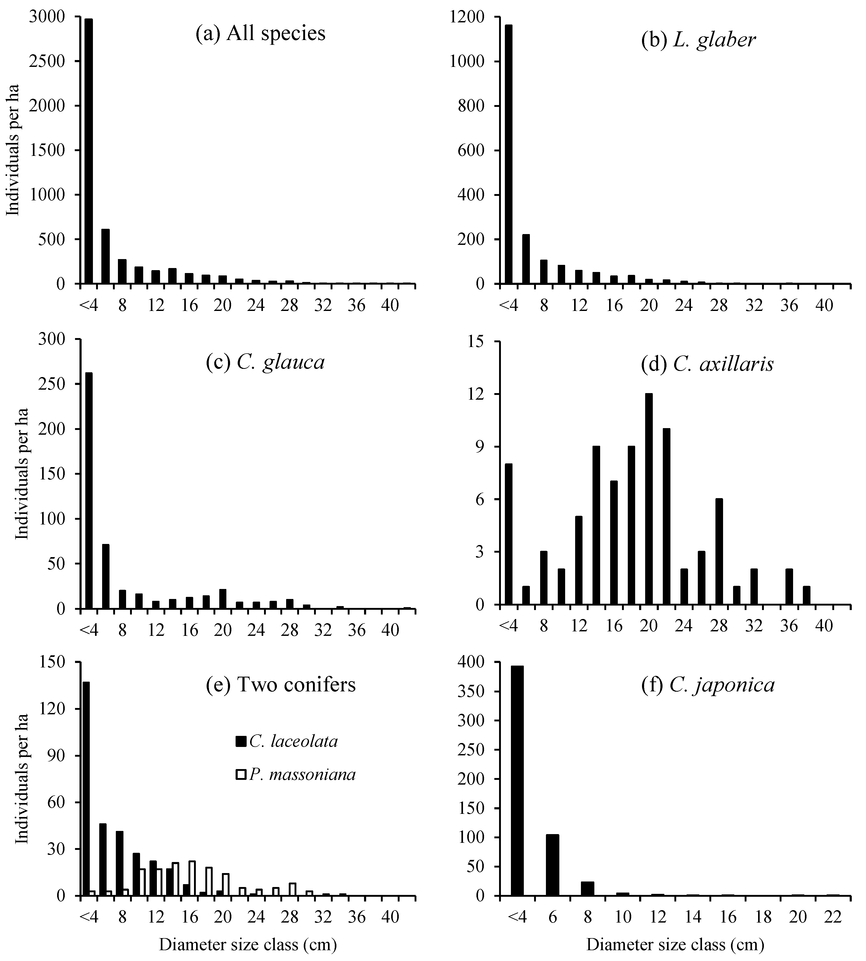
3.1. Stand Characteristics

When the individuals with a dbh ≥ 1 cm were counted, the 1 ha forest investigated contained 4797 stems, which belonged to 73 species, 55 genera, and 38 families. For stems with a dbh ≥ 4 cm, stand density was 1831 stems ha−1 from 45 species. Within the forest, BA amounted to 22.9 m2 ha−1 for all stems with a dbh ≥ 1 cm and 21.6 m2 ha−1 for all stems with a dbh ≥ 4 cm. Average dbh and height were 9.6 cm and 8.3 m for all stems with a dbh ≥ 4 cm, respectively. The largest in the plot was C. glauca at 42 cm in dbh and the tallest tree was Castanea henryi (Skan) Rehd. et Wils. at 26.1 m. The top six dominant species (dbh ≥ 1 cm) ranked by RIV were L. glaber, C. glauca, Pinus massoniana Lamb., Cleyera japonica Thunb., Cunninghamia lanceolata (Lamb.) Hook., and Choerospondias axillaris (Roxb.) Burtt et Hill. L. glaber and C. glauca trees accounted for 36.4% (based on dbh ≥ 1 cm) and 39.0% (dbh ≥ 4 cm) of RIV (Table 1 and Table 2).
Table 1. Density, basal area (BA), height, average diameter at breast height (dbh), frequency, and relative important value (RIV) of ten dominant species with a dbh ≥ 1 cm in a 1 ha evergreen broadleaved forest in China.
SpeciesDensity (Stems ha−1)BA (m2 ha−1)Height (m)dbh (cm)Frequency (%)RIV
L. glaber 18026.45.55.49425.3
C. glauca 4733.85.55.86211.1
P. massoniana1463.112.616.5457.2
C. japonica5290.63.73.3576.6
C. lanceolata3031.25.86.0515.7
C. axillaris832.311.518.4385.3
Loropetalum chinense (R. Br.) Oliver1850.13.32.5473.2
Eurya muricata Dunn1810.12.72.1463.1
Phyllostachys edulis (Carrière) J. Houz.941.112.212.292.5
C. henryi261.212.122.5162.5
Other 63 species9753.04.64.59527.5
Total 73 species479722.96.15.5100100.0
Table 2. Density, basal area (BA), height, average diameter at breast height (dbh), frequency, and relative important value (RIV) of ten dominant species with dbh ≥ 4 cm in a 1 ha evergreen broadleaved forest in China.
SpeciesDensity (Stems ha−1)BA (m2 ha−1)Height (m)dbh (cm)Frequency (%)RIV
L. glaber 6415.98.210.09026.4
C. glauca 2113.78.310.85012.6
P. massoniana1433.112.616.64510.2
C. lanceolata 1661.17.68.7427.4
C. axillaris752.312.019.2377.1
C. japonica1370.45.25.9345.2
P. edulis901.112.512.593.8
C. henryi261.212.122.4163.3
Quercus fabri Hance270.510.915.3192.5
Sassafras tzumu (Hemsl.) Hemsl.210.712.419.6142.3
Other 35 species2941.66.68.38119.2
Total 45 species183121.68.39.6100100.0
A reversed J shape for dbh distribution was found for all stems of the stand, where saplings (dbh < 4 cm) amounted to 2966 stems and accounted for 62.0% of total stems (Figure 2a). Dominant evergreen broadleaved woody species at a late succession stage (L. glaber and C. glauca showed reverse J-shaped distributions (Figure 2b,c,e), while early successional species (P. massoniana and C. axillaris) exhibited unimodal dbh distribution. The shrub species C. japonica had an L-shaped distribution (Figure 2f). L. glaber, C. glauca, C. lanceolata, and C. japonica had a large number of saplings (Figure 2b,c,e,f), however P. massoniana and C. axillaris lacked saplings in the understory layer (Figure 2d–e).
Figure 2. Distribution of diameter at breast height (dbh) size classes (at 2 cm intervals) for all woody species (a); two broadleaved evergreen tree species (L. glaber (b) and C. glauca (c)); a deciduous tree species (d); two coniferous tree species (e) and an evergreen shrub species (f).
Forests 06 00650 g002
Based on the total height of all stems, 62.4% of stems from 66 species were in the understory, while 13.1% of stems from 25 species were in the overstory of the forest. A similar vertical pattern was observed for dominant species, with the exception of P. massoniana and C. axillaris (Table 3).
Table 3. Characteristics of six dominant species and the stand as a whole (dbh ≥ 1 cm) at different vertical layers in a 1 ha evergreen broadleaved forest on the Dashanchong Forest Farm, China.
SpeciesIndividuals (Stems ha−1)Mean dbh (cm)Mean Height (m)
OMUOMUOMU
L. glaber 191527108414.36.42.312.16.93.3
C. glauca 8611727019.87.12.513.26.83.4
P. massoniana11036016.212.3-13.58.3-
C. lanceolata 2412415513.17.93127.23.3
C. japonica29043712.85.42.812.25.93.2
C. axillaris52201120.614.23.513.38.23.1
6 species465914195716.472.512.86.93.3
Total6301174299316.06.92.512.96.93.2
O, M, and U are abbreviations of overstory, midstory, and understory.

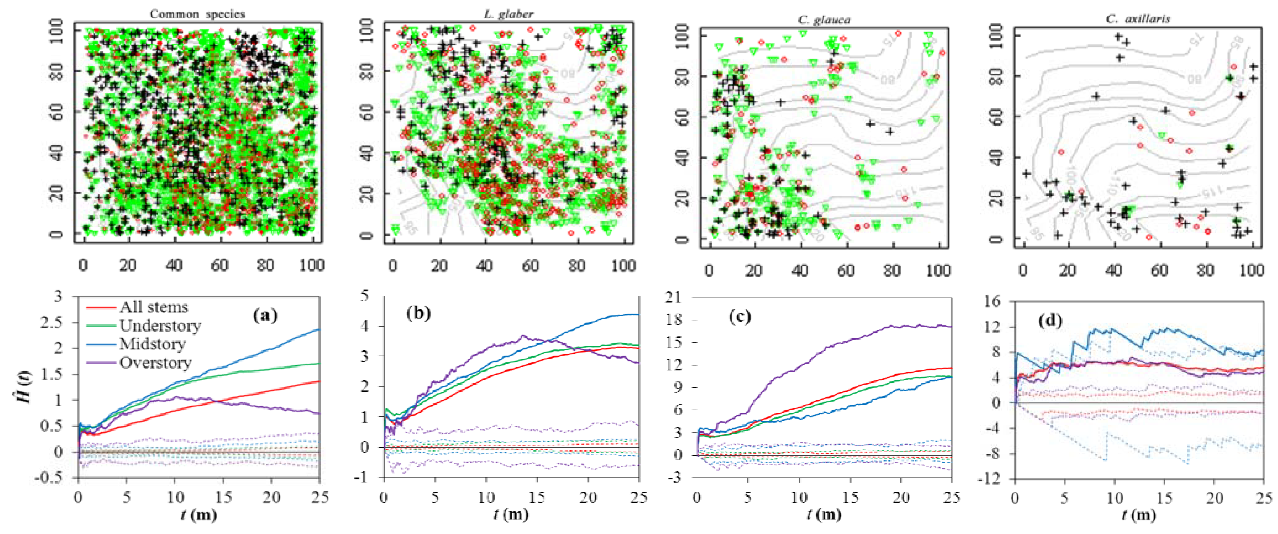
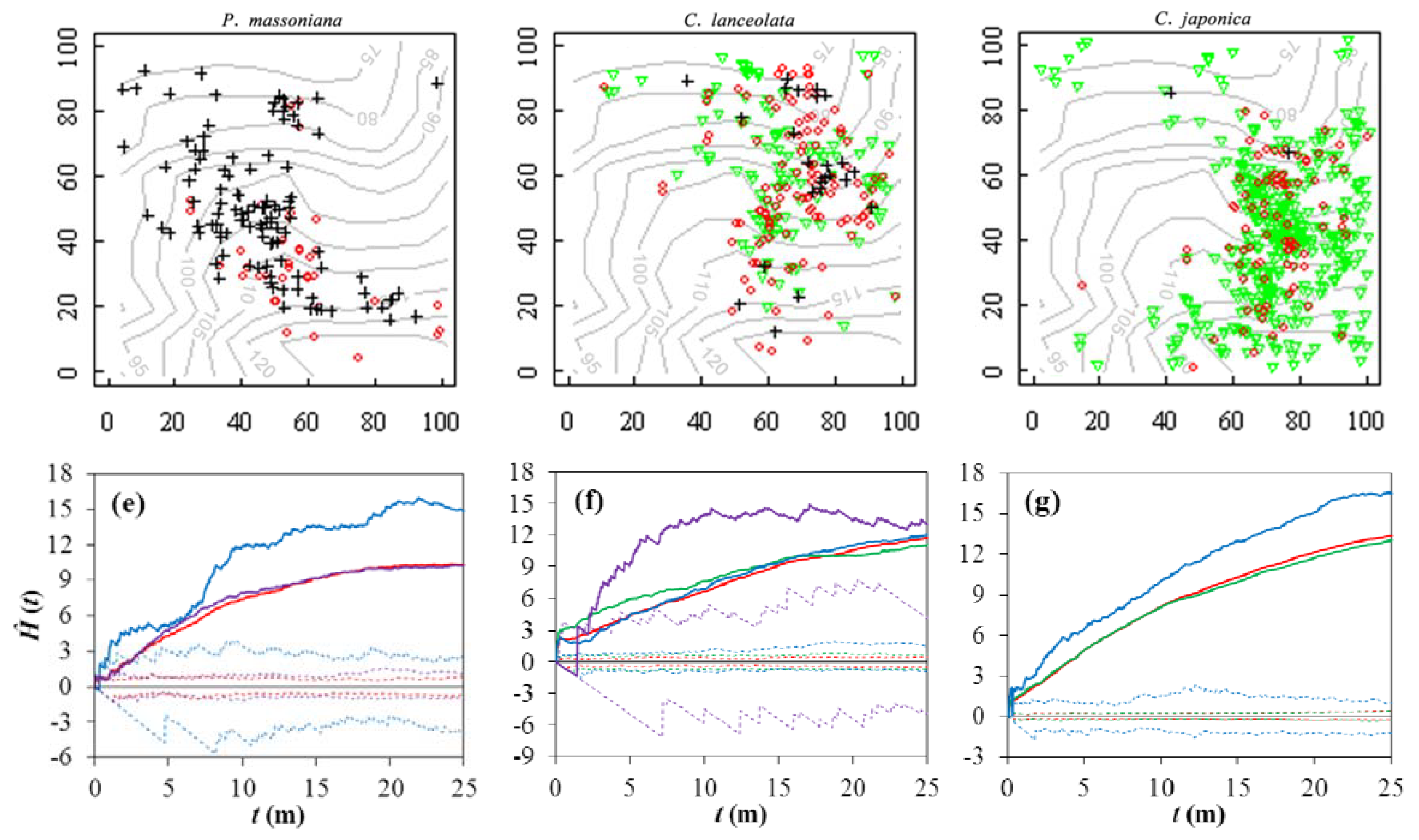
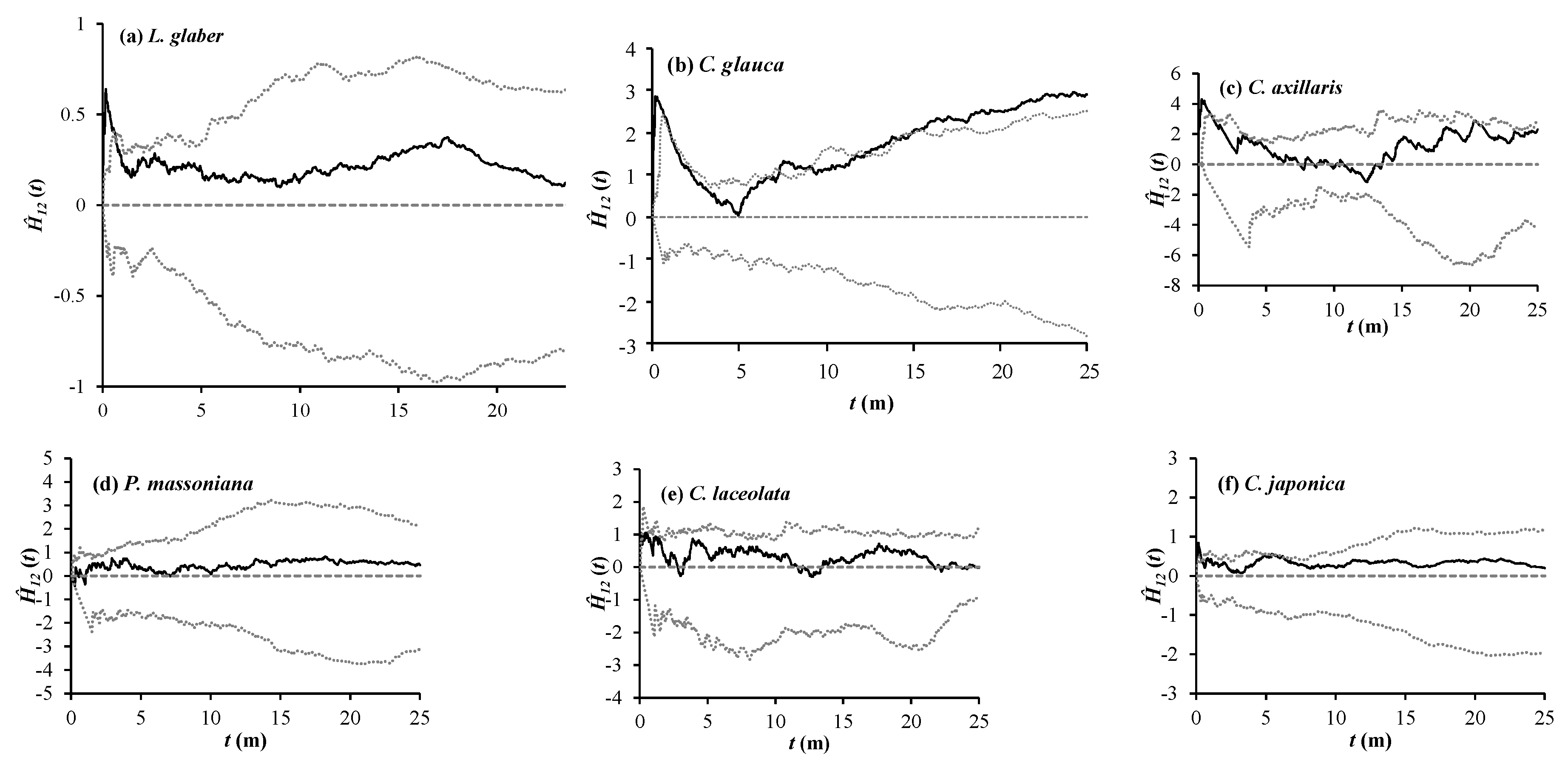
3.2. Spatial Patterns

Significant aggregation was observed for the stems (dbh ≥ 1) of 62 common species (excluding 11 rare species) in the whole stand or each layer across a 25 m distance (Figure 3). The aggregation intensity varied across vertical layers, with a higher degree of aggregation in the midstory layer and a lower degree in the overstory layer (Figure 3a).
Six dominant species also showed aggregated spatial patterns over the whole and different spatial scales, except the overstory of C. lanceolata, which showed random patterns at distances between 0 and 1 m (Figure 3b–g). Obviously, the intensity tended to increase with the distance for the stems of entire stands and the dominant six species, although some changes were found for C. axillaris trees and some overstory trees (e.g., L. glaber or stand).
Figure 3. Visual distribution maps and spatial patterns of all species and the six dominant species for all stems as well as stems at different vertical layers in the subtropical broadleaved evergreen forest plot on Dashanchong Forest Farm, China. The green triangle, red circle and black cross denote understory, middle-story, and overstory woody species, respectively. The solid lines denote Ĥ (t) values and dashed lines are the upper and lower limits of the 95% confidence envelope of Ĥ (t) generated by 999 computations of Monte Carlo (where t is distance). (a) all common species of the community; (b) L. glaber; (c) C. glauca; (d) C. axillaris; (d) P. massoniana; (e) C. laceolata; and (f) C. japonica.
Forests 06 00650 g003aForests 06 00650 g003b

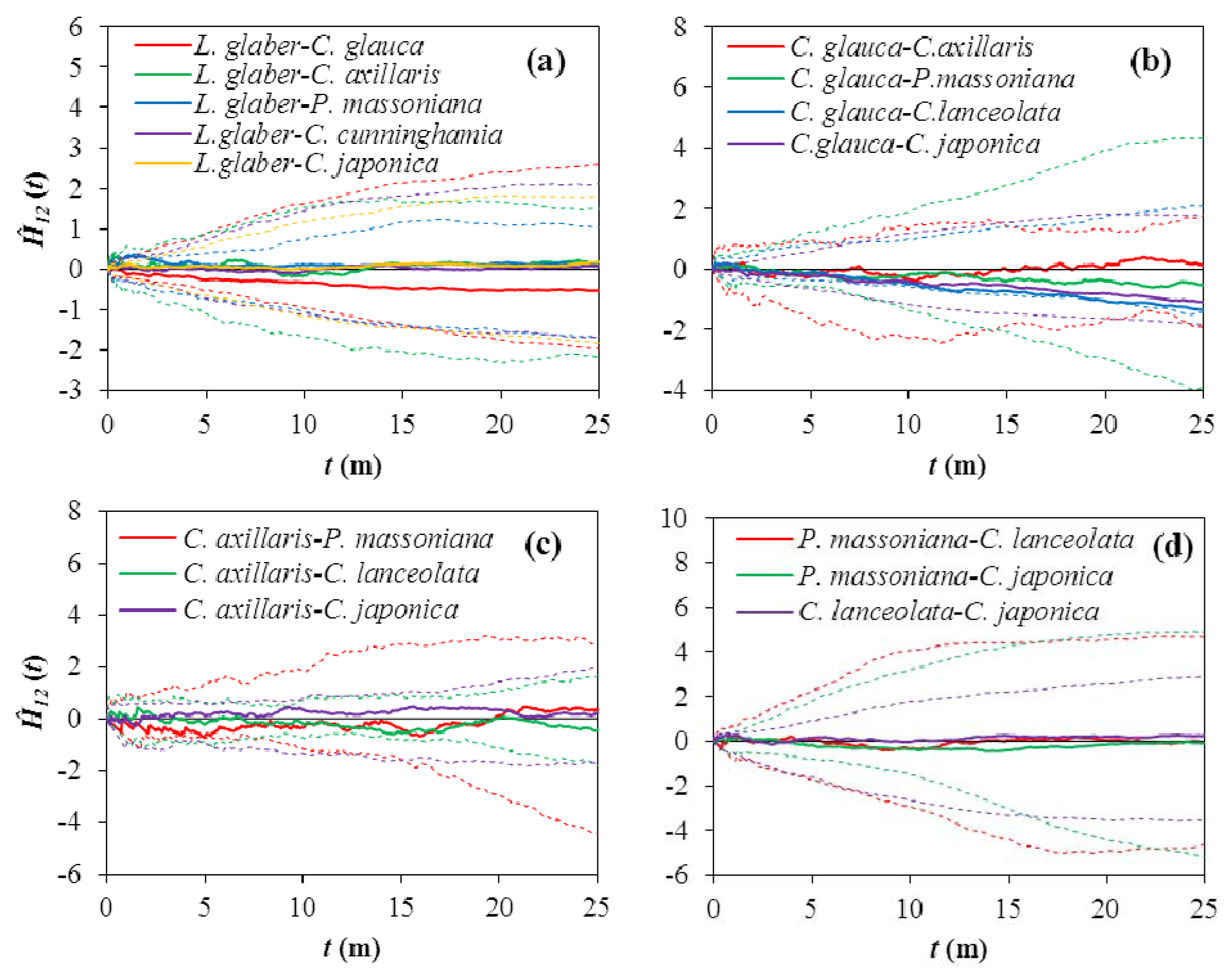
3.3. Spatial Associations

The interspecies spatial associations were independent between the six dominant species across all scales (Figure 4). Within each species, only conifers showed an independent pattern of spatial association between overstory and understory individuals. For the broadleaved species, intraspecific associations between overstory and understory individuals were spatially independent at long distances, while positive interactions were detected at short distances between 0 and 1 m for L. glaber (Figure 5a) and C. axillaris (Figure 5c) and less than 0.2 m for C. japonica (Figure 5f). For C. glauca, however, the relationships between overstory and understory individuals fluctuated and a significant attraction occurred at three distances, i.e., 0–1 m, 7–10 m and > 12 m (Figure 5b).
Figure 4. Spatial associations between the six dominant species in a subtropical broadleaved evergreen forest plot on Dashanchong Forest Farm, China. Solid lines represent Ĥ12 (t) values and dashed lines are the upper and lower limits of the 95% confidence envelope of Ĥ (t) generated by 999 computation of Monte Carlo (where t is the distance).
Forests 06 00650 g004
Figure 5. Spatial associations between overstory and understory stems for the six dominant species on the subtropical broadleaved evergreen forest plot on Dashanchong Forest Farm, China. Solid lines represent Ĥ12 (t) values and dashed lines are the upper and lower limits of the 95% confidence envelope of Ĥ (t) generated by 999 computations of Monte Carlo (where t is the distance).
Forests 06 00650 g005

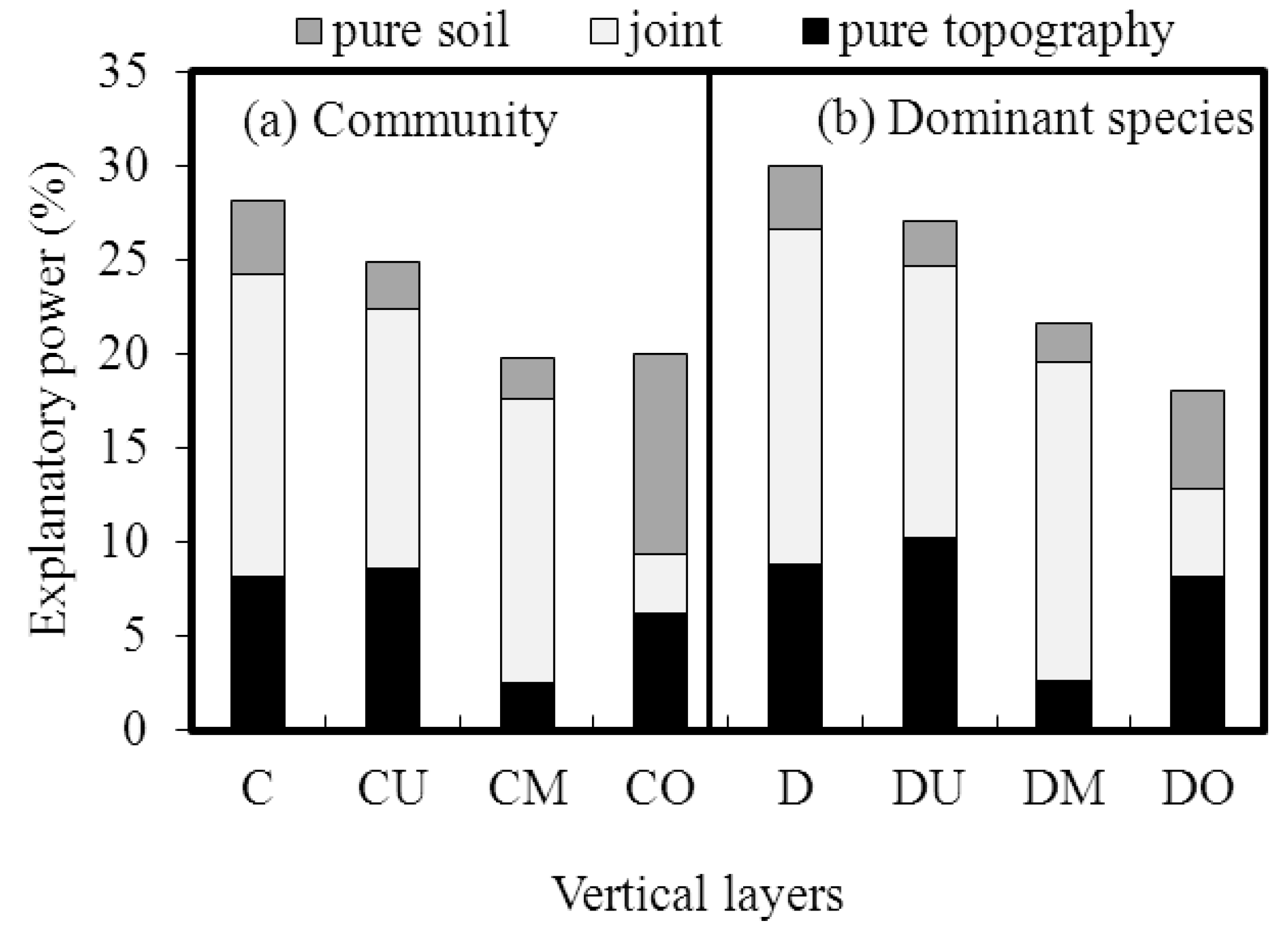
3.4. Contributions of Topographic and Soil Variables

At a stand level (Figure 6a), at least 20% of spatial variation in different layers could be explained by topography and soil. Over 50% of the explained variation could be related to the joint effects of topography and soil except for in the overstory. The relative contribution of pure soil was less than pure topography in the understory and midstory layers, while the reverse was observed in the overstory layer. For the six dominant species (Figure 6b), topographic and soil variables in total accounted for 29.9% of variation and the explanation power decreased from understory (27.0%) through midstory (21.6%) to overstory (18.1%). Meanwhile, topography contributed more than soil at each layer. Pure topography made the greatest contribution to the understory layer (10.3%), yet the explanation power of pure soil was the highest for the overstory layer.
Figure 6. Contribution of soil and topographic factors to variation in species abundance within the subtropical broadleaved forest plot on Dashanchong Forest Farm, China. “Pure soil”, “pure topography”, and “joint” represent the variation explained by pure soil, pure topography, or both topographic and soil variables together, respectively. C, CU, CM, and CO represent the whole stand, understory, midstory, and overstory of the forest, D, DU, DM, and DO represent all stems of dominant species and their corresponding layers.
Forests 06 00650 g006

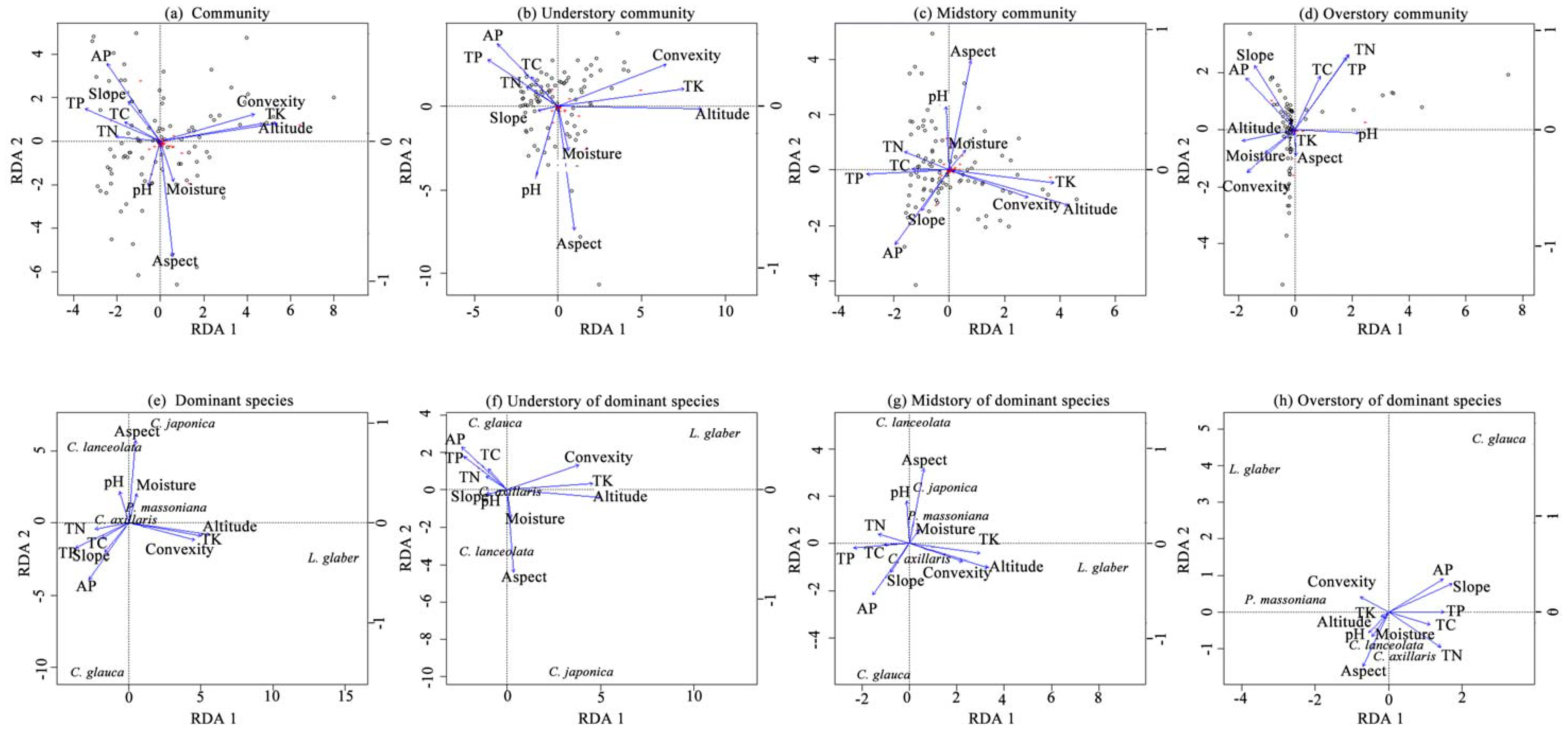
3.5. Main Driving Variables Across Vertical Layers

Aspect, altitude, AP, and TK were the important factors in determining species assembly for the understory and midstory of entire stands and the six dominant species (Figure 7). TN and slope were the important factors for overstory individuals and dominant species (Figure 7d,h). A significant correlation was found between soil and topographic factors. TK was positively correlated with convexity and altitude while AP was negatively correlated to aspect and positively to slope. For each dominant species, L. glaber was positively related to convexity, TK, and altitude. C. glauca was negatively related to aspect and positively related to AP and slope. C. japonica and C. lanceolata were positively correlated with aspect. However, C. axillaris and P. massoniana showed less correlation with the measured environmental factors because they were distributed closely at ordinate origin but overstory P. massoniana negatively related to TP (Figure 7h).
Figure 7. Canonical redundancy (RDA) plots of the whole stand and dominant species within the subtropical broadleaved forest plot on Dashanchong Forest Farm, China, displaying total layer together and each vertical layer separately. The black circle and the red crosses represent the location of subplots and species, respectively.
Forests 06 00650 g007

4. Discussion

4.1. Stand Characteristics and Regeneration

The 1 ha forest investigated in this study had 4797 stems (dbh ≥ 1cm) from 73 species of 55 genera and 38 families, which supports reports that subtropical evergreen broadleaved forest contained a high diversity of woody species [1,6,23]. Current floristic composition could yield some insights into the past successional process [37]. The presence of C. lanceolata as a dominant species indicated that the forest was developed on the site after clear-cutting of C. lanceolata plantation and the trees mainly originated from re-sprouting of some remaining stumps. Due to space and light availability at the early stage after harvest, the pioneer light-demanding species (e.g., coniferous species P. massoniana and deciduous species C. axillaris) invaded and became the dominant species in the forest. Canopy closure after a period of succession created favorable conditions for the immigration and recruitment of shade-tolerant species and then the evergreen broadleaved species L. glaber and C. glauca gradually came to dominate the forest.
Stand structure characteristics (i.e., dbh size distribution and vertical layer division) in the forests also reflect stand succession dynamics and regeneration capacity [42]. The reversed J-shape dbh distribution and distinct vertical layers in the forest of this study exhibited a typical feature of uneven-aged and multi-species forests [23,37]. A large number of saplings (2996 individuals with dbh between 1 and 4 cm) indicated that the forest had a high regeneration capacity. As shade-tolerant and late successional species, L. glaber and C. glauca had about 45% saplings in the understory and exhibited the reversed J-shape dbh distribution. Thus, evergreen broadleaved species showed great regeneration capacity and would be able to maintain their dominance in the future forest. However, early successional and shade-intolerant species (P. massoniana and C. axillaris) had fewer saplings (0.4%) in the understory and showed a unimodal dbh distribution pattern. Unfavorable site conditions for seedling establishment and survival were obvious for early successional species so these species would disappear in the future forest. Hence, our results indicated the forest in this study was close to the late successional stage of subtropical evergreen broadleaved forests and the dominant evergreen broadleaved species would be consolidated in the forest if no high intensity disturbances occurred.

4.2. Implications of Spatial Patterns and Associations for Species Assembly

The findings of aggregated spatial patterns for the entire stand and dominant species in the forest of this study (Figure 3) are consistent with the reports from species-rich tropical forests [43], evergreen broadleaved forests in subtropical China [6,17,23], and temperate forests [11]. Aggregated spatial distribution is a widespread pattern in naturally regenerated forests [36,44] and could be attributed to numerous factors [11,13] that affect species immigration and extinction [1]. Biotic processes (seed dispersal, regeneration strategy, and competition) [9,11] and abiotic filter processes (habitat heterogeneity) [30] are considered as the two major driving processes.
Spatial associations between different species and between understory saplings and overstory conspecific species could offer some information about seed dispersal [9,45] and regeneration strategies [11] of specific species in the forests. The shade-tolerant and late successional species, L. glaber and C. glauca, have strong sprouting abilities [22] and their chestnut seeds are of heavy weight with limited dispersal range [10]. Thus, seedlings and sprouts of L. glaber and C. glauca grew well and were very common in the forest and their understory saplings were positively associated with the overstory parent trees on a fine scale lower than 1 m (Figure 5a,b). With regard to early successional and light-demanding species, P. massonina has wind-dispersed seeds while C. axillaris has heavy berry seeds with predation-dependent dispersal strategies. Their shade-intolerant seedlings could not survive in the understory, therefore, fewer understory saplings of C. axillaris were found and were positively associated with the overstory parent trees. The shrub species C. japonica grew well in the midstory and understory, and showed a greater aggregation intensity than other dominant species. The aggregated spatial pattern resulted from their limited dispersal capacity resisted by high neighborhood trees.
Changes in aggregation intensity between vertical layers are survival strategies or adaptation mechanisms of a population. Large trees usually reduce aggregation intensity to obtain adequate resources from the environment and to ensure a species distribution in suitable habitat [46]. Previous studies found that different species could establish themselves and survive in different habitats, which depended on many factors such as heterogeneous light distribution [21] and soil and topographic variation [44]. P. massonina and C. axillaris are light-demanding species. Young individuals of these species can only survive if seeds are distributed in gaps; therefore, light resource plays an important role in these species assembly. In contrast, light is not an obvious limiting factor for other species that were related with topographic and soil factors. For example, L. glaber and C. glauca showed obvious habitat preferences and a greater tendency to aggregate in suitable habitat during the mature stage by means of habitat filtering. Generally, spatial distribution patterns are primarily affected by the functional traits of a species on a small scale, while habitat heterogeneity is considered to be the most likely explanation for larger scales [47].

4.3. Relative Contribution of Topography and Soil

Quantitative RDA analysis in this study supported the widely accepted findings that topography and soil affected species composition and spatial distribution [48]. Our results showed that topographic and soil variables could explain 28.1% and 29.9% of spatial distribution of entire stands and dominant species, respectively. Species were aggregated along environmental gradients due to habitat preference [14]. However, the effects of topography and soil differed among vertical layers. In this study, the contribution of topography and soil decreased from the understory to the overstory, and only soil explained more variation regarding the midstory individuals of dominant species. In terms of dominant species, AP was the critical soil variable, while TN was the only significantly positive correlation with the distribution of overstory species. Both topography and soil together, topography as well as pure topography contributed the most to the understory individuals and dominant species in the stands. Species were affected by certain limiting environmental factors across life stages and only certain individuals could access the overstory layer, suggesting that habitats had filtering effects on species distribution in the forests [48].
Furthermore, topographic variables explained more variation than soil variables for each layer of the entire stand and dominant species, except for the overstory in the stand. This result was identically scaled (10 m) with the Dinghushan Nature Reserve evergreen broadleaved forest [48]. At least 53.4% of contribution of total topography and soil came from their joint effects, with the exception of 36.1% for dominant species overstory variation, indicating that topography affects spatial distribution of soil moisture [14] and nutrients [15], and that topographically structured soil is crucial for plants. Our results showed that L. glaber prefers to grow in the position of high elevation and convex slope with high TK concentration whereas C. glauca prefers to gather in the position of high slope with high AP concentration (Figure 7). Meanwhile, elevation, slope position, and convexity affect soil drainage, soil depth, and nutrient concentrations. Thus, variation in topography and soil provide suitable conditions for different species; this is the basis for the mechanism of niche differentiation [44].
In this study, unexplained variances occurred more than 70%, indicating that habitat heterogeneity does not have a decisive influence on species assembly. Other non-correlated associations with measured habitat spatial aggregation processes may affect species assembly. Some underlying variations in biotic processes have been overlooked; these include shade-tolerance, species regeneration strategy, and some unmeasured environmental variables (e.g., light resources), which emphasize the importance of processes in niche areas [49]. Alternatively, it could be the result of pure spatial variation, such as dispersal limitation and other stochastic processes that are more associated with neutral processes [50].

5. Conclusions

The community investigated was a stable structured uneven-aged, multi-species forest with a known good regeneration capacity. Aggregated spatial distribution was the dominant pattern, and independent associations were the primary relationship between dominant species or overstory and understory individuals of conspecific species. Topographic and soil variables played different roles at different vertical layers, and critical environmental variables varied among vertical layers, indicating that habitats have filtering effects on species assembly. Multiple processes affect species distribution, and further non-correlation with habitat spatial aggregation processes, such as shade-tolerance, regeneration strategy, and seed dispersal limitation of a species, have more influence than habitat heterogeneity. This information concerning species assembly in a Chinese subtropical evergreen broadleaved forest could help decision-makers to design appropriate strategies for forest management and biodiversity conservation. In practice, tree species selection for mixture plantation establishment, suitable site arrangement for target species planting, and selective thinning for natural regeneration are essential for sustainable forest management based on close-nature forest management conception.

Acknowledgments

This study was supported by the Program of State Forestry Special Fund for Public Welfare Sectors of China (201304317), the National Natural Science Foundation of China (31170426), and the New Century Excellent Talents Program (NCET-06-0715). We would like to thank the following post-graduates for their assistance in field investigations: Hao Yi, Xuding Wen, Fei Cui, Gangwei Fan, Dan Yang, Limei Zou, Yuqing Xu, Xu Zhang, and Jianjun Zhou. We would also like to thank the staff of the administration office of Dashanchong Forest Farm for their local support.

Author Contributions

Conception and design of experiments: W.X. Implemented the experiments: L.Z., J.L., P.L., X.D. and X.F. Analyzed the data: L.Z., J.L. and W.X. Contributed reagents, materials, and analysis tools: W.X. Wrote the paper: L.Z., W.X., J.L., P.L. and C.P.

Conflicts of Interest

The authors declare no conflict of interest.

References

  1. Bruelheide, H.; Böhnke, M.; Both, S.; Fang, T.; Assmann, T.; Baruffol, M.; Bauhus, J.; Buscot, F.; Chen, X.Y.; Ding, B.Y.; et al. Community assembly during secondary forest succession in a Chinese subtropical forest. Ecol. Monogr. 2011, 81, 25–41. [Google Scholar] [CrossRef] [Green Version]
  2. Connell, J.H.; Slatyer, R.O. Mechanisms of succession in natural communities and their role in community stability and organization. Am. Nat. 1977, 111, 1119–1144. [Google Scholar] [CrossRef]
  3. Veblen, T.T.; Ashton, D.H.; Schlegel, F.M. Tree regeneration strategies in a lowland Nothofagus-dominated forest in south-central Chile. J. Biogeogr. 1979, 6, 329–340. [Google Scholar] [CrossRef]
  4. Zenner, E.K.; Lahde, E.; Laiho, O. Contrasting the temporal dynamics of stand structure in even- and uneven-sized Picea abies dominated stands. Can. J. For. Res. 2011, 41, 289–299. [Google Scholar] [CrossRef]
  5. Baraloto, C.; Hardy, O.J.; Paine, C.E.T.; Dexter, K.G.; Cruaud, C.; Dunning, L.T.; Gonzalez, M.A.; Molino, J.F.; Sabatier, D.; Savolainen, V.; et al. Using functional traits and phylogenetic trees to examine the assembly of tropical tree communities. J. Ecol. 2012, 100, 690–701. [Google Scholar] [CrossRef]
  6. Li, L.; Huang, Z.L.; Ye, W.H.; Cao, H.L.; Wei, S.G.; Wang, Z.G.; Lian, J.Y.; Sun, I.F.; Ma, K.P.; He, F. Spatial distributions of tree species in a subtropical forest of China. Oikos 2009, 118, 495–502. [Google Scholar] [CrossRef]
  7. Manabe, T.; Nishimura, N.; Miura, M.; Yamamoto, S. Population structure and spatial patterns for trees in a temperate old-growth evergreen broad-leaved forest in Japan. Plant Ecol. 2000, 151, 181–197. [Google Scholar] [CrossRef]
  8. Shen, G.C.; He, F.L.; Waagepetersen, R.; Sun, I.F.; Hao, Z.Q.; Chen, Z.S.; Yu, M.J. Quantifying effects of habitat heterogeneity and other clustering processes on spatial distributions of tree species. Ecology 2013, 94, 2436–2443. [Google Scholar] [CrossRef] [PubMed]
  9. Seidler, T.G.; Plotkin, J.B. Seed dispersal and spatial pattern in tropical trees. PLoS Biol. 2006, 4, e344. [Google Scholar] [CrossRef] [PubMed]
  10. Condit, R.; Ashton, P.S.; Baker, P.; Bunyavejchewin, S.; Gunatilleke, S.; Gunatilleke, N.; Hubbell, S.P.; Foster, R.B.; Itoh, A.; LaFrankie, J.V.; et al. Spatial patterns in the distribution of tropical tree species. Science 2000, 288, 1414–1418. [Google Scholar] [CrossRef] [PubMed]
  11. Hou, J.H.; Mi, X.C.; Liu, C.R.; Ma, K.P. Spatial patterns and associations in a Quercus- Betula forest in northern China. J. Veg. Sci. 2004, 15, 407–414. [Google Scholar]
  12. Chen, L.Z.; Chen, W.L. Chinese Degraded Ecological System Research; Science Press: Beijing, China, 1995. [Google Scholar]
  13. Yamada, T.; Zuidema, P.A.; Itoh, A.; Yamakura, T.; Ohkubo, T.; Kanzaki, M.; Tan, S.; Ashton, P.S. Strong habitat preference of a tropical rain forest tree does not imply large differences in population dynamics across habitats. J. Ecol. 2007, 95, 332–342. [Google Scholar] [CrossRef]
  14. Harms, K.E.; Condit, R.; Hubbell, S.P.; Foster, R.B. Habitat associations of trees and shrubs in a 50-ha neotropical forest plot. J. Ecol. 2001, 89, 947–959. [Google Scholar] [CrossRef]
  15. John, R.; Dalling, J.W.; Harms, K.E.; Yavitt, J.B.; Stallard, R.F.; Mirabello, M.; Hubbell, S.P.; Valencia, R.; Navarrete, H.; Vallejo, M.; et al. Soil nutrients influence spatial distributions of tropical tree species. Proc. Natl. Acad. Sci. USA 2007, 104, 864–869. [Google Scholar] [CrossRef] [PubMed]
  16. Legendre, P.; Mi, X.; Ren, H.B.; Ma, K.; Yu, M.; Sun, I.F.; He, F. Partitioning beta diversity in a subtropical broad-leaved forest of China. Ecology 2009, 90, 663–674. [Google Scholar] [CrossRef] [PubMed]
  17. Zhang, Z.; Hu, G.; Zhu, J.; Ni, J. Aggregated spatial distributions of species in a subtropical karst forest, southwestern China. J. Plant Ecol. 2013, 6, 131–140. [Google Scholar] [CrossRef]
  18. Chang, L.W.; Zelený, D.; Li, C.F.; Chiu, S.T.; Hsieh, C.F. Better environmental data may reverse conclusions about niche-and dispersal-based processes in community assembly. Ecology 2013, 94, 2145–2151. [Google Scholar] [CrossRef] [PubMed]
  19. Zhang, C.Y.; Zhao, Y.Z.; Zhao, X.H.; Klaus, V.G. Species-Habitat Associations in a Northern Temperate Forest in China. Silva Fenn. 2012, 46, 501–519. [Google Scholar]
  20. Comita, L.S.; Condit, R.; Hubbell, S.P. Developmental changes in habitat associations of tropical trees. J. Ecol. 2007, 95, 482–492. [Google Scholar] [CrossRef]
  21. Hao, Z.; Zhang, J.; Song, B.; Ye, J.; Li, B. Vertical structure and spatial associations of dominant tree species in an old-growth temperate forest. For. Ecol. Manag. 2007, 252, 1–11. [Google Scholar] [CrossRef]
  22. Qi, C.J. Hunan Vegetation; Hunan Science and Technology Press: Changsha, China, 1990; pp. 51–341. [Google Scholar]
  23. Xiang, W.H.; Liu, S.H.; L, X.D.; Frank, S.C.; Tian, D.L.; Wang, G.J.; Deng, X.W. Secondary forest floristic composition, structure, and spatial pattern in subtropical China. J. For. Res. 2013, 18, 111–120. [Google Scholar] [CrossRef]
  24. Yasmi, Y.; Broadhead, J.; Enters, T.; Genge, C. Forestry Policies, Legislation and Institutions in Asia and the Pacific: Trends and Emerging Needs for 2020, Asia-Pacific Forestry Sector Outlook Study II; Food and Agriculture Organization of the United Nations: Bangkok, Thailand, 2010. [Google Scholar]
  25. Diaci, J. Nature-Based Forestry in Central Europe: Alternatives to Industrial forestry and Strict Preservation; Biotechnical Faculty, University of Ljubljana: Ljubljana, Slovenia, 2006. [Google Scholar]
  26. Lai, J.S. Species Habitat Associations and Species Coexistence on Evergreen Broad-Leaved Forest in Gutianshan, Zhejiang. Ph.D. Thesis, Chinese Academy of Science, Beijing, China, June 2008. [Google Scholar]
  27. Xie, Y.B.; Ma, Z.P.; Yang, Q.S.; Fang, X.F.; Zhang, Z.G.; Yan, E.R.; Wang, X.H. Coexistence mechanisms of evergreen and deciduous trees based on topographic factors in Tiantong region, Zhejiang Province, eastern China. Biodivers. Sci. 2012, 20, 159–167. [Google Scholar]
  28. Zhao, L.J.; Xiang, W.H.; Li, J.X.; Deng, X.W.; Liu, C. Composition, structure and phytogeographic characteristics in a Lithocarpus glaber-Cyclobalanopsis glauca forest community in mid-subtropical China. Sci. Silvae Sin. 2013, 49, 10–17. [Google Scholar]
  29. Tonon, G.; Panzacchi, P.; Grassi, G.; Gianfranco, M.; Cntoni, L.; Bagnaresi, U. Spatial dynamics of late successional species under Pinus nigra stands in the northern Apennines (Italy). Ann. For. Sci. 2005, 62, 669–679. [Google Scholar] [CrossRef]
  30. Lan, G.Y.; Hu, Y.H.; Cao, M.; Zhu, H. Topography related spatial distribution of dominant tree species in a tropical seasonal rain forest in China. For. Ecol. Manag. 2011, 262, 1507–1513. [Google Scholar] [CrossRef]
  31. Bao, S.D. Soil and Agricultural Chemistry Analysis; China Agriculture Press: Beijing, China, 2000. [Google Scholar]
  32. Galindo-Jaimes, L.; González-Espinosa, M.; Quintana-Ascencio, P.; García-Barrios, L. Tree composition and structure in disturbed stands with varying dominance by Pinus spp. in the highlands of Chiapas, Mexico. Plant Ecol. 2002, 162, 259–272. [Google Scholar] [CrossRef]
  33. Ripley, B.D. Modelling spatial patterns. J. R. Stat. Soc. B 1977, 39, 172–212. [Google Scholar]
  34. Haase, P. Spatial pattern analysis in ecology based on Ripley’s K-function: Introduction and methods of edge correction. J. Veg. Sci. 1995, 6, 575–582. [Google Scholar] [CrossRef]
  35. Ripley, B.D. Test of randomness for spatial point patterns. J. R. Stat. Soc. B 1979, 41, 368–374. [Google Scholar]
  36. Besag, J.; Diggle, P.J. Simple Monte Carlo test for spatial pattern. J. Appl. Stat. 1977, 26, 327–333. [Google Scholar] [CrossRef]
  37. Salas, C.; LeMay, V.; Núñez, P.; Pacheco, P.; Espinosa, A. Spatial patterns in an old-growth Nothofagus obliqua forest in south-central Chile. For. Ecol. Manag. 2006, 231, 38–46. [Google Scholar] [CrossRef]
  38. Baddeley, A.; Turner, R. Spatstat: An R package for analyzing spatial point patterns. J. Stat. Softw. 2005, 12, 1–42. [Google Scholar]
  39. Core Development Team R. A Language and Environment for Statistical Computing; R Foundation for Statistical Computing: Vienna, Austria, 2009. Available online: http://www.R-project.org (accessed on 22 April 2006).
  40. Peres-Neto, P.R.; Legendre, P.; Dray, S.; Borcard, D. Variation partitioning of species data matrices: Estimation and comparison of fractions. Ecology 2006, 87, 2614–2625. [Google Scholar] [CrossRef] [PubMed]
  41. Oksanen, J.; Kindt, R.; Legendre, P.; O’Hara, B.; Simpson, G.L.; Solymos, P.; Stevens, M.H.H.; Wagner, H. Vegan: Community Ecology Package, R package version 1.14-12; Available online: http://vegan.r-forge.r-project.org/ (accessed on 3 June 2008).
  42. Takahashi, K.; Homma, K.; Vetrova, V.P.; Florenzev, S.; Hara, T. Stand structure and regeneration in a Kamchatka mixed boreal forest. J. Veg. Sci. 2001, 12, 627–634. [Google Scholar] [CrossRef]
  43. Plotkin, J.B.; Potts, M.D.; Leslie, N.; Manokaran, N.; LaFrankie, J.; Ashton, P.S. Species- area curves, spatial aggregation, and habitat specialization in tropical forests. J. Theor. Biol. 2000, 207, 81–99. [Google Scholar] [CrossRef] [PubMed]
  44. He, F.L.; Legendre, P.; LaFrankie, J.V. Distribution patterns of tree species in a Malaysian tropical rain forest. J. Veg. Sci. 1997, 8, 105–114. [Google Scholar] [CrossRef]
  45. Liu, Q.J. Structure and dynamics of the subalpine coniferous forest on Changbai mountain, China. Plant Ecol. 1997, 132, 97–105. [Google Scholar] [CrossRef]
  46. Hubbell, S.P. Neutral theory and the evolution of ecological equivalence. Ecology 2006, 87, 1387–1398. [Google Scholar] [CrossRef] [PubMed]
  47. Yuan, Z.; Gazol, A.; Wang, X.; Lin, F.; Ye, J.; Bai, X.; Li, B.; Hao, Z. Scale specific determinants of tree diversity in an old growth temperate forest in China. Basic Appl. Ecol. 2011, 12, 488–495. [Google Scholar] [CrossRef]
  48. Lin, G.J.; Stralberg, D.; Gong, G.Q.; Huang, Z.L.; Ye, W.H.; Wu, L.F. Separating the effects of environment and space on tree species distribution: From population to community. PLoS One 2013, 8, e56171. [Google Scholar] [CrossRef] [PubMed]
  49. Jones, M.M.; Tuomisto, H.; Borcard, D.; Legendre, P.; Clark, D.B.; Olivas, P.C. Explaining variation in tropical plant community composition: Influence of environmental and spatial data quality. Oecologia 2008, 155, 593–604. [Google Scholar] [CrossRef] [PubMed]
  50. Punchi-Manage, R.; Getzin, S.; Wiegand, T.; Kanagaraj, R.; Savitri Gunatilleke, C.V.; Nimal Gunatilleke, I.A.U.; Wiegand, K.; Huth, A.; Zuidema, P. Effects of topography on structuring local species assemblages in a Sri Lankan mixed dipterocarp forest. J. Ecol. 2013, 101, 149–160. [Google Scholar] [CrossRef]

