Assessment of Wooded Area Reduction by Airborne Laser Scanning

Abstract

Airborne Laser Scanning (ALS) data hold a great deal of promise in monitoring the reduction of single trees and forests with high accuracy. In the literature, the canopy height model (CHM) is the main input used frequently for forest change detection. ALS also has the key capability of delivering 3D point clouds, not only from the top canopy surface, but also from the entire canopy profile and also from the terrain. We investigated the use of two additional parameters, which exploit these capabilities for assessing the reduction of wooded area: Slope-adapted echo ratio (sER) and Sigma₀. In this study, two ALS point cloud data sets (2005 and 2011) were used to calculate Digital Surface Model (DSM), sER, and Sigma₀ in 1.5 km² forest area in Vorarlberg, Austria. Image differencing was applied to indicate the change in the three difference models individually and in their combinations. Decision trees were used to classify the area of removed trees with the minimum mapping unit of 13 m². The final results were evaluated by a knowledge-based manual digitization using completeness and correctness measures. The best result is achieved using the combination of sER and DSM, namely a correctness of 92% and a completeness of 85%.

1. Introduction

Forests are an important factor in maintaining the balance in the Earth system. However, the ecological processes are often affected by human activity [1]. In order to control the change of forests under the impacts of deforestation, wind throw, and diseases, it is required for forest managers to apply techniques supporting monitoring and updating forest information regularly. In situ forest inventory and remote sensing technologies are in use for detecting and monitoring these changes. Remote sensing, as one of these techniques, has proven its ability in change detection, automatically, efficiently, and consistently, especially for large areas, this also requiring less manual labor.

Optical remote sensing is a good choice to detect changes of forests as demonstrated in different studies [2,3,4,5]. However, optical acquisition techniques are limited by clouds if they are below the platform. Photograhic techniques additionally provide little information in cast shadow, as well as topographic shadow areas, providing little or no texture and, thus, lead to lower accuracy there. Furthermore, the varying shadow conditions for different acquisition times limit an automatic large area derivation of forest changes.

The image matching technique shows its potential use in forestry [6,7]. Photogrammetric imagery can also be exploited for gaining 3D point clouds [8]. Nevertheless, the limitation of this technique is that information is restricted to the point cloud of the upper canopy and, thus, does not provide ground height [9]. The image-based point cloud quality depends on factors like ground sampling distance, radiometric image resolution, stereo-parameters, viewing geometry, sun-angle, and amount of shadows [9].

With the advantage of penetrating the canopy through small gaps, Airborne Laser Scanner (ALS) is a potential technique for monitoring vegetation changes. Being an active technique, ALS emits its own energy for sensing and is consequently not affected by the ambient illumination (cast shadows, shadows of high clouds). Using 3D point clouds from ALS, the change in both coverage and height can be detected [10,11]. Moreover, not only dense forests, but even single trees can be detected from dense point clouds [12], which can be used to estimate forest biomass [13,14] and generate 3D tree models [15,16].

Although ALS data holds a high promise in vegetation change detection, thus far, research using multi-temporal ALS to detect forest change cover has not yet been fully explored. Yu et al. [17] detected harvested trees using two small footprint, high sampling density ALS acquisitions based on image differencing. Three-dimensional canopy height models (CHM) were calculated for both data sets using raster-based algorithms. The major change of CHM at the same pixel was acquired by a threshold value. They reported that 61 out of 83 field-checked harvested trees were detected automatically. The undetected trees were mainly smaller trees. St-Onge et al. [18] also used the threshold of CHM difference of two medium density LiDAR data acquired in 1998 and 2003 to identify new canopy gaps and assess height growth. With the same data Vepakomma et al. [19] expanded their study in accessing the feasibility of small footprint LiDAR to map the canopy gap expansions and canopy gap closures for the conservation zone of Quebec. Vastaranta et al. [20] developed a ∆CHM method for canopy change detection of snow-damaged trees by applying bi-temporal LiDAR data for the period 2006–2010. Næsset and Gobakken [21] estimated a boreal forest growth over two years by using canopy metrics, i.e., measures of spatial distribution of the acquired point cloud. Nyström et al. [22] employed histogram matching to calibrate the metrics in order to reduce the difference between two ALS datasets and produce change imagery. They controlled the changes by partial and complete tree removal in selected plots. Hollaus et al. [23] assessed the changes in growing stock of 160 km² mountain forest by two ALS datasets. The model was established with 184 FI (forest inventory) plots.

The above-mentioned studies used the differences found in (two) datasets over a forest area. Alternatively, processes in the forest can be detected using only one dataset by the traces they leave in the site. For example, Mücke et al. [24] used full-waveform ALS data, obtained under leaf-off conditions to detect fallen trees. Here, an echo width model was derived based on the point cloud and normalized echo heights in order to delineate downed stems. Lindberg et al. [25] and Nyström et al. [26] contributed two different methods highlighting the potential of high density ALS data to detect wind-thrown trees under forest canopy. Lindberg et al. [25] used a line template matching method applied directly to the ALS point cloud (69 points/m²), while Nyström et al. [26] used the difference between two elevation models created from the same high density ALS data to detect wind-thrown trees.

In this research, we investigate the ability of forest reduction detection from two different ALS datasets by using image differencing [27]. In comparison to Nyström, who applied histogram matching to account for different sensor characteristics, our aim is to find features of LiDAR point clouds, that are, as much, as possible independent of the sensor characteristics. Unlike other studies mentioned above, our hypothesis is that forest reduction up to individual trees can be observed by the three LiDAR derived models: Digital Surface Model (DSM), Slope-adaptive Echo Ratio (sER), and “Sigma₀” (a local roughness measure), as well as their combinations. Our primary interest is, thus, not to demonstrate that ALS can detect forest changes as this was done before [17,22]. Rather, we are interested in finding robust methods in the presence of different ALS mission parameters. The study is done for a mountain forest in Vorarlberg, Austria. Two epochs were acquired with six years difference between the data acquisitions. The DSMs demonstrate the change in height and, thus, indicate that tall objects were removed. sER demonstrates the change in vertical penetrability and indicates that layered objects (e.g., understory and canopy) were removed. Sigma₀ demonstrates the change in the vertical dispersion of the points and indicates that objects distributed in height (e.g., trees, bushes) were removed. Using these variables, in different combination, the forest reduction is derived. The results are accessed with their accuracy by using the completeness and correctness measure. All the processes are supported by OPALS [28] and ArcGIS software.

2. Material and Method

2.1. Study Area

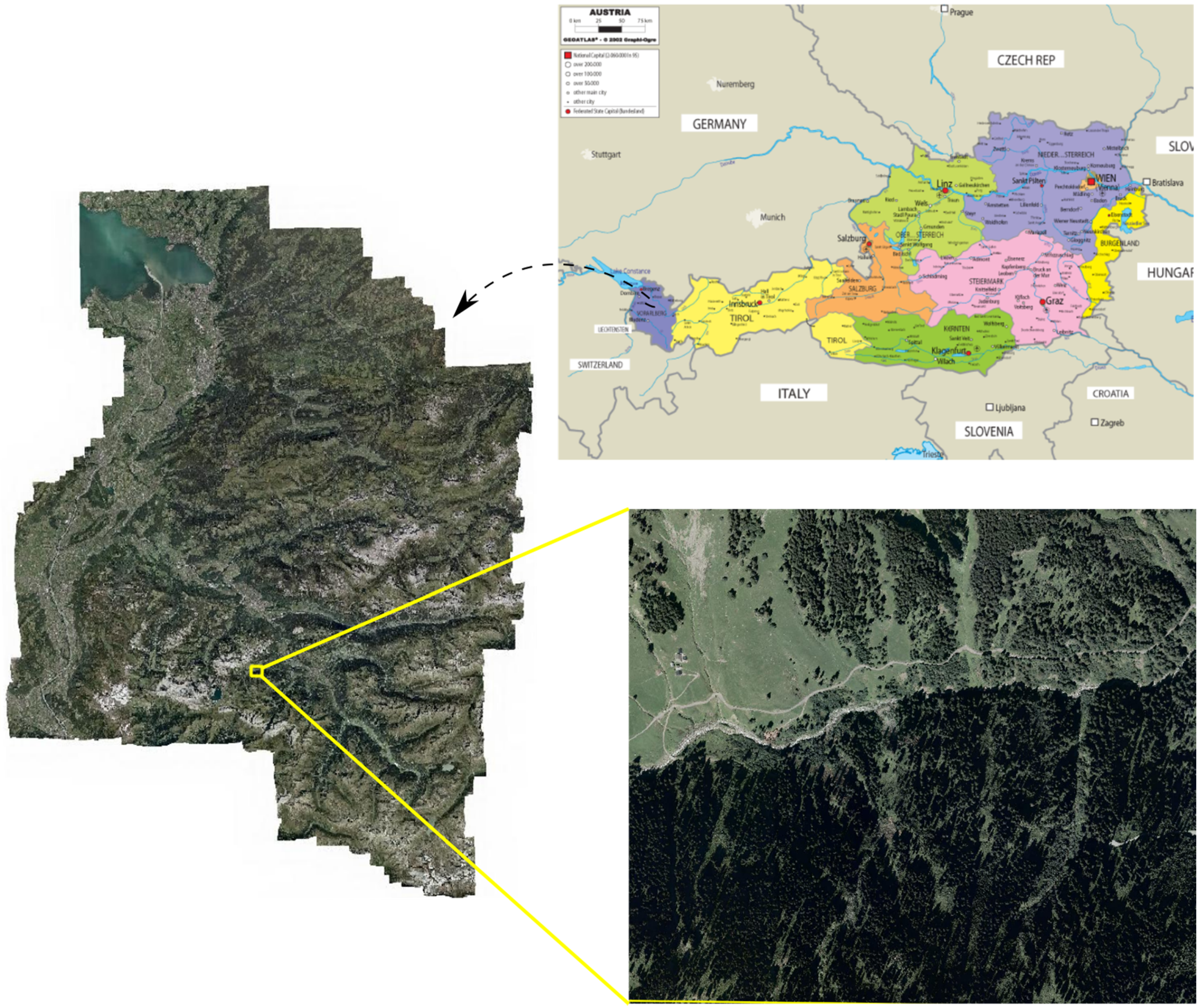
Study area is located in the south of Vorarlberg province, Austria, centered on lat. N 47°04′12″, long. E 9°49′12″ (Figure 1). The total covered area is about 1.5 km² of mountainous region, with the elevations ranges from 1225 m above sea level (a.s.l) in the valleys, to a maximum of 1786 m a.s.l. In general, in this area, approx. 24% is covered by forest and the dominating tree species is Norway spruce (Picea abies). The forests in the study area are managed by the Stand Montafon Forstfonds (http://stand-montafon.at/forst), which operates the local forest inventory. Based on this inventory the tree heights vary between approximately 6 m to 42 m, with the mean height of 27.5 m and the standard deviation is 6.8 m [29]. Due to the topography the majority of the forests in the study area have a protection function against natural hazards, i.e., snow avalanches. Therefore, exploitations of single trees or group of trees are foreseen in the forest management plan, meaning clear cuttings of larger areas are not allowed.

Figure 1. Study area (Orthophoto: office of survey and geoinformation from Vorarlberg, Austria, Political Map of Austria: GEOATLAS.com.).

Figure 1. Study area (Orthophoto: office of survey and geoinformation from Vorarlberg, Austria, Political Map of Austria: GEOATLAS.com.).

2.2. Data

The two ALS data sets were provided by the local office of survey and geo-information from the federal state of Vorarlberg, and are subsets of the official federal state-wide ALS data acquisition campaigns. The ALS data sets were acquired in 2005 and 2011 using an Airborne Laser Terrain Mapper systems (ALTM 1225) and a Trimble Harrier 56 system, respectively. The study area is covered by two flight strips for the first ALS acquisition and three flight strips for the second acquisition. All ALS data sets were acquired under snow-free and leaf-off conditions and were available as georeferenced 3D-point clouds. In Table 1, the relevant sensor characteristics of used ALS systems are summarized.

Table 1. Summary of sensor characteristics of the applied ALS systems.

Sensor Characteristics	Sensors
	Acquisition Year 2005	Acquisition Year 2011
	Optech ALTM 1225	Trimble Harrier 56
Beam divergence	0.3 mrad	<0.5 mrad
Max scan angle (from nadir)	20°	30°
Wavelength	1064 nm	1064 nm
Pulse repetition frequency	<25 kHz	160 kHz
Sensor type	Discrete	Full waveform
Average point density	6 echos/m2	24 echos/m2

Table 1. Summary of sensor characteristics of the applied ALS systems.

Sensor Characteristics	Sensors
	Acquisition Year 2005	Acquisition Year 2011
	Optech ALTM 1225	Trimble Harrier 56
Beam divergence	0.3 mrad	<0.5 mrad
Max scan angle (from nadir)	20°	30°
Wavelength	1064 nm	1064 nm
Pulse repetition frequency	<25 kHz	160 kHz
Sensor type	Discrete	Full waveform
Average point density	6 echos/m2	24 echos/m2

2.3. Reference Data

The reference data was derived, based on image interpretation of aerial orthophotos [30] with additional use of 3D point cloud viewing of the raw ALS data. Orthophotos with a spatial resolution of 0.12 m (2012) and 0.5 m (2005) are used to overview the forest cover status. Using additionally various visualizations of the ALS data, such as 3D point cloud visualization in FugroViewer software, nDSM values of the same pixels in two epochs, each single 1 m² pixel was evaluated and digitized. Due to border effects, a tree crown can be influenced in the DSMs by a slightly different shape. Therefore, small changes of very few m² were not considered as relevant and the therefore, the minimum mapping area was set to 13 m². This process took roughly 100 h. For the 223 digitized polygons, the minimum polygon area is 13 m² and the maximum area is 2351 m², the average size of a harvested polygon is 152 m² and the standard deviation is 289 m². The mean height of harvested polygons is 30.8 m and the standard deviation is 8.2 m. The final digitized output is converted into a binary format with a raster size of 1 × 1 m² that is used for accuracy assessment.

2.4. Method

In this study 3D ALS point clouds are used as the basis for deriving the following parameters, which are used for delineating harvested trees:

• DSM,
• sER, and
• Sigma₀.

For forest change detection the DSMs are an important input because they describe the height changes of the top most canopy surface. This means a decrease of the DSM indicates the loss of trees. To derive the DSMs from the two ALS data sets, the land cover dependent method described, in Hollaus et al. [31], is applied. This method uses the strengths of different algorithms for generating the final DSM by using surface roughness information to combine two DSMs, which are calculated based on the highest echo within a raster cell, and on moving least squares (mls) interpolation with a plane as functional model (i.e., a tilted regression plane fitted through the k-nearest neighbors). For smooth areas (e.g., roof planes, streets, short grassland), noise reduction by moving least squares interpolation is exploited, whereas for rough surfaces (e.g., canopy surface, building edge) the highest point within a raster cell is used (DSM(X, Y)_max). The input for moving least squares interpolation is a subset of the point cloud (highest points within 0.5 m rater cells), which ensures that the interpolated surface goes through the tree tops. The derived final DSMs have a spatial resolution of 1 m.

More formally, the DSM calculation runs in the following way (Here we use the trinary operator c ? r₁: r₂. Its value depends on the condition c. If c is TRUE, the result is r₁, otherwise the result is r₂.).

z[DSM (Xi, Yi)]2005 = z[σz(Xi, Yi)]2005 < 0.5 or not z[DSM (Xi, Yi)max]2005 ? z[DSM (Xi, Yi)mls]2005:

z[DSM (Xi, Yi)max]2005

z[DSM (Xj, Yj)]2011 = z[σz(Xj, Yj)]2011 < 0.5 or not z[DSM (Xj, Yj)max]2011 ? z[DSM (Xj, Yj)mls]2011:

z[DSM (Xj, Yj)max]2011

ΔDSM (X, Y) = DSM²⁰¹¹ (X, Y) − DSM²⁰⁰⁵(X, Y)

(1)

The sER is a measure that describes the vertical point distribution and thus the penetrability of the surface [32,33]. The echo ratio (not slope-adaptive) is defined as the ratio between the number of neighboring echoes in a fixed search distance, measured in 3D (a sphere, n_3D, see appendix for exact definition), and all echoes located within the same search distance in 2D (a vertical cylinder, n_2D). To guarantee a correct ER on steep slopes, the search radius of the sphere (r_2D) has to be extended considering the slope (r_3D = r_2D/cos(α)) (i.e., dividing the initial 3D search distance by the cosine of the slope). Thus, the derived ER is the slope-adaptive echo ratio, sER.

$$s\text{ER}=\frac{{\text{n}}_{3\text{D}}\left(\text{r}/\cos \text{α}\right)}{{\text{n}}_{2\text{D}}\left(\text{r}\right)}\times 100$$

(2)

The sER is computed for each echo in the first processing step and shows for continuous and impenetrable surface (i.e., ground and roof surfaces) values of 100% and for tree canopy points of lower value. For further analyses, the sER is aggregated in 1 m cells using the max value within each cell. The modules opalsEchoRatio and opalsCell were used for this computation.

ΔsER (X, Y) = sER²⁰¹¹(X, Y) − sER²⁰⁰⁵(X, Y)

(3)

For the computation of Sigma₀, all echoes are used with a neighborhood size of the ten nearest neighbors. It is derived during the interpolation of a height model using the moving least squares approach. The standard deviation of the residuals in this interpolation is determined at each grid post. This provides a grid congruent with the interpolated heights. In each grid post, this value of Sigma₀ indicates how well all of the original points fit to the least squared plane. The grid width was 1 m.

ΔSigma₀ (X, Y) = Sigma₀²⁰¹¹(X, Y) − Sigma₀²⁰⁰⁵(X, Y)

(4)

As the decreases of the elevation of the canopy surface indicate the loss of trees, the DSM²⁰⁰⁵ is subtracted from the DSM²⁰¹¹. In addition to the elevation changes, the changes in the vertical echo distribution and penetrability described with the sER model and the changes of the surface roughness, represented by the Sigma₀ model, also indicate areas with lost (e.g., harvested) trees. Thus, difference models of the sER and the Sigma₀ models are also calculated. To use this information, it is assumed that the sER of point clouds have a lower value for trees than for open ground (e.g., removed trees) and for Sigma₀ it receives a higher value.

The thresholds for all change values (i.e., DSM, sER and Sigma₀) are assessed empirically. No primary maps of vegetated area were derived for the epochs. In other words, no maps of DSM, sER, and Sigma₀ were studied. Instead, we are searching directly for thresholds on the observed differences, thus, in ΔDSM, ΔsER, and ΔSigma₀.

All three data sets (ΔDSM, ΔsER, ΔSigma₀) indicate lost tree positions. Additionally, combinations of those input variables, for improving the accuracy of the final result, were investigated. Each pair and the triple of variables are used with newly determined empirical thresholds. The change results can be expected to show small errors, localized in single pixels or very small groups of pixels (i.e., along the border of trees or forests). This is caused by the accuracy of the acquired data (i.e., point density, georeferencing), as well as by the interpolation. The results are, therefore, converted into binary format for applying methods of binary mathematical morphology. Closing and then opening morphology with a circular kernel shape with a diameter of 1 and 2 pixels respectively are applied to all output raster datasets to reduce noise and to smooth object outlines. Finally, six change detection outputs were established: DSM only, sER only, Sigma₀ only, DSM combined with sER, sER combined with Sigma₀ and DSM, and sER and Sigma₀. Early in the analysis it became obvious, that the combination of DSM and Sigma₀ offers no increase of the achievable accuracy than the other pairs, thus, it was omitted.

Completeness (Comp) and correctness (Corr) [34] are used for the accuracy assessment of the final results.

$$\text{Comp}=\frac{\Vert \text{TP}\Vert }{\Vert \text{TP}\Vert +\Vert \text{FN}\Vert }$$

(5)

$$\text{Corr}=\frac{\Vert \text{TP}\Vert }{\Vert \text{TP}\Vert +\Vert \text{FP}\Vert }$$

(6)

The forest reduction area in the reference and change detection results are compared, where a true positive (TP) indicate the change in both datasets, false negative (FN) is labeled in the reference data but has no correspondence in the change detection results, and false positive (FP) is labeled in the change detection results and has no corresponding in the reference data.

3. Results and Discussion

The main properties of the primary models (DSM, sER and Sigma₀) are summarized in Table 2. Based on the empirical analyses, the thresholds for each of the different image (ΔDSM, ΔsER and ΔSigma₀ variables were found and summarized in Table 3. Figure 2 shows the harvested tree detection results of the three variables DSM, sER, and Sigma₀ independently, as well as the manual digitized reference map. As can be seen, the downed tree area was detected, more or less, correctly. However, the results are affected by salt-and-pepper type of noise. After applying image morphology operations, the Sigma₀ final results are still strongly affected by this and give the worst accuracy (Table 3) compared with the other two variables (Figure 3a–c).

Table 2. Minimum, maximum, mean, standard deviation of DSM, sER, and Sigma₀ in the different epochs.

	Min	Max	Mean	Std.dev
DSM2005(m)	1226.2	1817.1	1516.4	124.0
DSM2011(m)	1226.0	2022.1 1	1517.1	124.0
sER2005(%)	1.9	100.0	69.9	29.3
sER2011(%)	2.3	100.0	65.5	29.9
Sigma02005(m)	0.0	28.0	2.9	4.2
Sigma02011(m)	0.0	220.3 2	2.7	4.2

¹ This value is affected by gross errors. Excluding them leads to a max DSM of 1817.9; ² Excluding gross error the max Sigma₀²⁰¹¹ is 27.2.

Table 2. Minimum, maximum, mean, standard deviation of DSM, sER, and Sigma₀ in the different epochs.

	Min	Max	Mean	Std.dev
DSM2005(m)	1226.2	1817.1	1516.4	124.0
DSM2011(m)	1226.0	2022.1 1	1517.1	124.0
sER2005(%)	1.9	100.0	69.9	29.3
sER2011(%)	2.3	100.0	65.5	29.9
Sigma02005(m)	0.0	28.0	2.9	4.2
Sigma02011(m)	0.0	220.3 2	2.7	4.2

¹ This value is affected by gross errors. Excluding them leads to a max DSM of 1817.9; ² Excluding gross error the max Sigma₀²⁰¹¹ is 27.2.

Figure 2. Forest reduction based on the selected thresholds for the (a) DSM; (b) sER; (c) Sigma₀; and (d) Knowledge-based digitization.

Figure 2. Forest reduction based on the selected thresholds for the (a) DSM; (b) sER; (c) Sigma₀; and (d) Knowledge-based digitization.

Table 3. Threshold values and accuracy measures.

Change threshold	DSM (m)	sER (%)	Sigma0 (m)	Corr (%)	Comp (%)
ΔDSM	<−7.0	----	----	84.6	90.9
ΔsER	----	>30	----	87.5	87.1
ΔSigma0	----	----	<−7.0	38.6	56.8
ΔDSM and sER	<−2.0	>27	----	91.9	85.1
ΔsER and Sigma0	----	>27	<−2.0	90.9	80.8
ΔDSM and sER and Sigma0	<−2.0	>25	<−1.0	92.8	82.4
ΔDSM and sER and Sigma01	<−7.0	>30	<−7.0	96.4	38.2

¹ The result of this combination is not shown in the Figure 3.

Table 3. Threshold values and accuracy measures.

Change threshold	DSM (m)	sER (%)	Sigma0 (m)	Corr (%)	Comp (%)
ΔDSM	<−7.0	----	----	84.6	90.9
ΔsER	----	>30	----	87.5	87.1
ΔSigma0	----	----	<−7.0	38.6	56.8
ΔDSM and sER	<−2.0	>27	----	91.9	85.1
ΔsER and Sigma0	----	>27	<−2.0	90.9	80.8
ΔDSM and sER and Sigma0	<−2.0	>25	<−1.0	92.8	82.4
ΔDSM and sER and Sigma01	<−7.0	>30	<−7.0	96.4	38.2

¹ The result of this combination is not shown in the Figure 3.

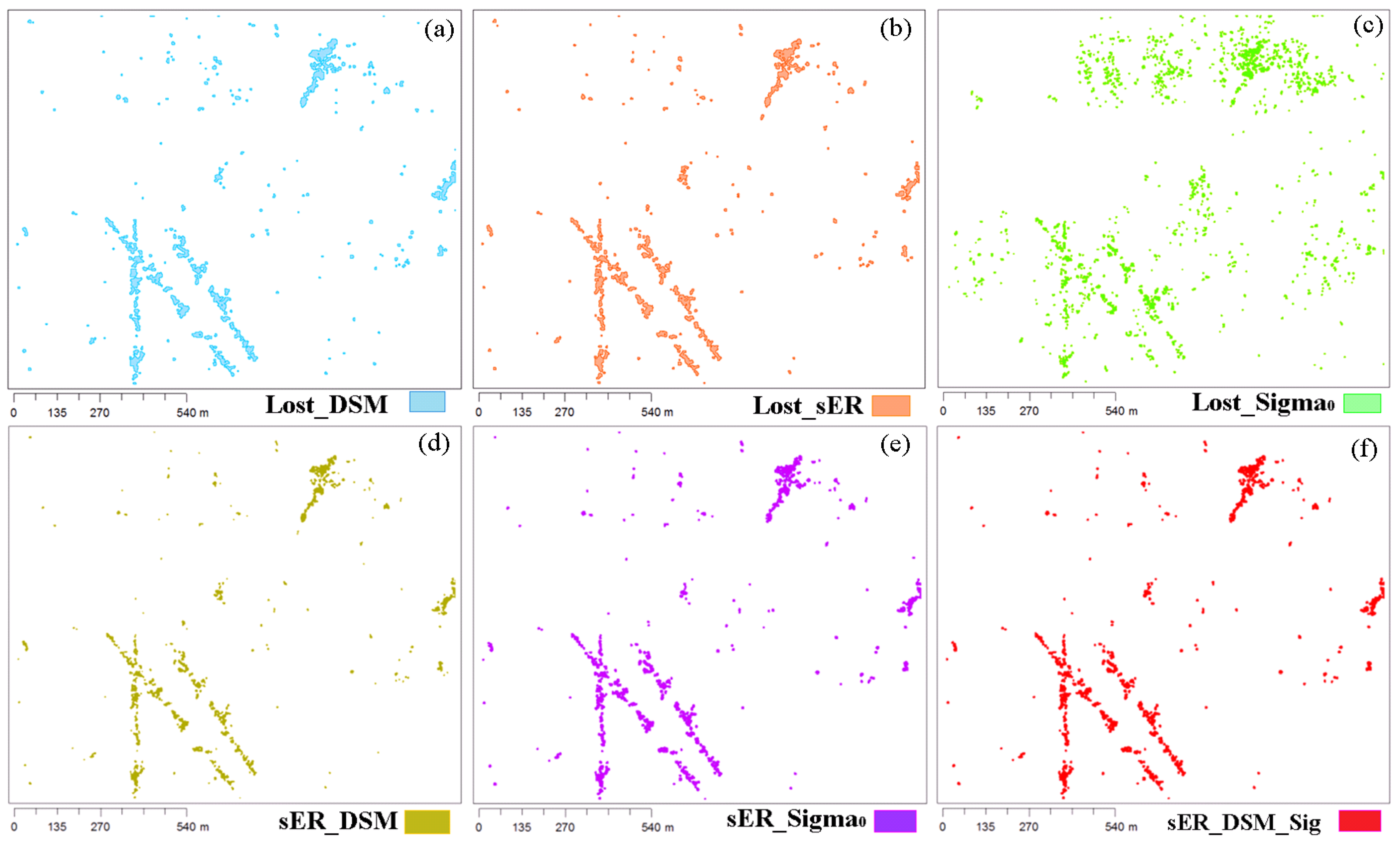
Figure 3. Final forest reduction after morphological operation (a) DSM; (b) Echo ratio; (c) Sigma₀; (d) Echo ratio and DSM; (e) Echo ratio and Sigma₀; (f) Echo ratio and DSM and Sigma₀.

Figure 3. Final forest reduction after morphological operation (a) DSM; (b) Echo ratio; (c) Sigma₀; (d) Echo ratio and DSM; (e) Echo ratio and Sigma₀; (f) Echo ratio and DSM and Sigma₀.

The limitations of DSM and Sigma₀ compared to sER are to detect the reduction of low trees. Using a threshold, which is too low in height change, the lost tree cover is easy to be mixed with the unchanged forest cover. Additionally, Sigma₀ may depend much more on flying parameters, such as the flying height, which influences the point density and consequently the Sigma₀ values. Regarding to sER, because sER is larger influenced by its neighborhood so it has an increased value for the lost trees in a larger area. This leads to a reduction in the capability of detecting lost trees in dense canopy regions.

In order to overcome the limitation of each variable, all variables are incorporated in combinations in order to achieve improved results. To acquire the threshold of each pair combination between ΔsER versus ΔDSM, ΔsER versus ΔSigma₀, and ΔDSM versus ΔSigma₀, a feature space (Figure 4) is used to distinguish changed areas. The area of change is in either case in the upper left part of the feature space. It deviates from the distribution of unchanged areas, which is centered on (0, 0). As stated above, the pair ΔDSM versus ΔSigma₀ does not show the discrimination in the feature space compared to other pairs, thus it is not used to detect changes. The median value of ΔDSM, ΔsER and ΔSigma₀ of the reference data also calculated and plotted into the feature space for delineating the threshold. From the feature space, the threshold for the ΔDSM and ΔsER combination (ΔDSM < −2 AND ΔsER > 27) and the ΔsER and ΔSigma₀ combination (ΔsER > 27 AND ΔSigma₀ < −2) are found, as a result, the accuracy of change detection is improved (Table 3, Figure 3). The former provides a correctness of 91.9% and completeness of 85.1% higher than the latter with a correctness of 90.9% and a Completeness of 80.8%. The combination of all three variables awards the highest correctness (92.8%) and a lower completeness (82.4%). As could be expected, using the original thresholds of the single variable classifications shows the highest correctness (96%) at the cost of a lower completeness (only 38.2%). The accuracy assessment of seven final change detection results is shown in Table 3.

Figure 4. Feature space of (a) ΔsER versus ΔSigma₀; (b) ΔsER versus ΔDSM. The red lines indicate the threshold values for change detection. Brighter colors denote a higher density of points (from blue, to green, to red). Red dots indicated the median value of ΔDSM, ΔsER, and ΔSigma₀ of the reference polygons.

Figure 4. Feature space of (a) ΔsER versus ΔSigma₀; (b) ΔsER versus ΔDSM. The red lines indicate the threshold values for change detection. Brighter colors denote a higher density of points (from blue, to green, to red). Red dots indicated the median value of ΔDSM, ΔsER, and ΔSigma₀ of the reference polygons.

Our final result achieved a accuracy (with a minimum mapping unit of 13 m²) compared to the research of Yu et al. [17], who detected 61 out of 83 harvested trees with an accuracy of 73.5%. St-Onge and Vepakomma [18] used canopy height differences to identify new gaps (especially fallen trees) and the minimum area criterion is 5 m². Their data has a density of 3 shots/m² in each epoch. Producer and user accuracies are similar to ours, although a bit higher (95%–98%). However, they apparently confirmed the existence of gaps in the reference (optical images) and the LiDAR result, but not the exact spatial location. Small edge localization errors and gap size differences between our reference and LiDAR result add to lower producer and user accuracy in our case. Additionally, the results of Nyström et al. [22] can be compared to our results. Their overall accuracy in detection is 88%, thus, somewhat lower than our result. However, in the forest-tundra ecotone, in which their study is set, the geometric signal of changes is lower than in ours in the case of taller trees.

Analyzing the Sigma₀ values of the different missions indicated that they depend more strongly on the parameters of the data acquisition. Two point clouds of a single tree are displayed and visualized in 3D, and it is realized that the point distributions and point densities of the same tree are different. This will influence the value of the Sigma₀ results. Therefore, in this study, surface roughness (Sigma₀) alone is not a reasonable measure to detect forest change.

In Figure 4, there are some sER median values for reference polygons located under the selected threshold. It is explained that, in some dense tree positions, the sER values of downed trees are influenced by points of the other surrounding trees.

In the case of deciduous forests with a dense canopy surface and fully developed foliage, there is no penetration into the canopy and to the ground. It leads to high sER and small Sigma₀ values for trees. Harvested trees can be better detected with ΔDSM in this case. On the other hand, errors in vertical geo-referencing directly influence the DSM and, therefore, ΔDSM, but it does not affect sER and Sigma₀. Therefore, the combination of sER and DSM will provide the highest quality in detecting the reduction of wooded area.

Scan frequency, flying altitude, scan angle, acquisition time (i.e., leaf-on, leaf-off), and applied methods for preprocessing have an influence on data quality [35,36]. Based on the applied method for DSM calculation, the influences of these properties are minimized [31].

For a detailed assessment of forest biomass changes it is important to differentiate between forest growth and exploitation. For the quantification of the exploitation, detailed information about reduced (i.e., harvested trees) forest area is required. The assessment of forest growth is based on changes in the DSM, which requires robust methods to derive DSM from the ALS point clouds that are, as much as possible, independent from sensor characteristics and data acquisition settings [31]. To minimize influences originating from georeferencing issues, advanced georeferencing, including a strip adjustment, is normally required [23]. For the assessment of the biomass change, regression models can be applied to the individual data sets. For the calibration of these regression models [37], reference data, e.g., forest inventory data, are required. Finally, the biomass change can be derived from the differences between the individual biomass maps.

4. Conclusions

Using the image differencing method, a traditional pixel-based change detection method was applied to detect reduction of forest area. In this study, we used the three variables DSM, slope adaptive echo ratio (sER), and Sigma₀, derived from two different ALS data sets, to detect downed trees in a forest. While many studies have, thus far, used DSM and its change, we found that sER is a good single predictor for tree cover change. sER is a local measurement, which means that global height differences, e.g., ALS block geo-referencing problems, do not influence the assessment. It is also noted that the threshold value for sER (Table 2) did not change as much as for DSM and Sigma₀ in the combined classifications.

The incorporations of two or more variables always improved the quality of detection results, only the combination of DSM and Sigma₀ does not provide an improvement. This study opens up a new application of discrete return ALS data in forest change detection and, therefore, in forest management. We conclude that the best results were achieved using sER change with additional consideration of DSM change, namely a correctness of 92% and a completeness of 85%.