Article

Mapping Temporal Dynamics in a Forest Stream Network—Implications for Riparian Forest Management

1
Department of Forest Ecology and Management, Swedish University of Agricultural Science, Umeå 901 83, Sweden
2
Skogforsk, the Forestry Research Institute of Sweden, Uppsala Science Park, Uppsala 751 83, Sweden
*
Author to whom correspondence should be addressed.
These authors contributed equally to this work.
Forests 2015, 6(9), 2982-3001; https://doi.org/10.3390/f6092982
Submission received: 1 June 2015 / Revised: 12 August 2015 / Accepted: 25 August 2015 / Published: 28 August 2015
(This article belongs to the Special Issue Forest Management and Water Resources in the Anthropocene)

Abstract

:
This study focuses on avoiding negative effects on surface waters using new techniques for identifying wet areas near surface waters. This would aid planning and designing of forest buffer zones and off-road forestry traffic. The temporal variability in the geographical distribution of the stream network renders this type of planning difficult. A field study was performed in the 68 km2 Krycklan Catchment to illustrate the variability of a boreal stream network. The perennial stream length was 140 km while the stream length during high-flow conditions was 630 km. Comparing the field-measured stream network to the network presented on current maps showed that 58% of the perennial and 76% of the fully expanded network was missing on current maps. Similarly, cartographic depth-to-water maps showed that associated wet soils constituted 5% of the productive forest land during baseflow and 25% during high flow. Using a new technique, maps can be generated that indicate full stream networks, as well as seasonally active streams and associated wet soils, thus, forestry planning can be performed more efficiently and impacts on surface waters can be reduced.

1. Introduction

Today, forestry is often performed using various forest machinery and forest soils can be subjected to traffic several times during a rotation period. Because of the increasing need for forest bioenergy to meet green energy targets including the EU Renewable Energy Directive, harvest intensity is expected to increase in many countries [1,2]. This will place additional pressure on boreal water quality [3,4], for instance by increased off-road forestry traffic. Driving with heavy machinery on forest soils can cause rutting and soil compaction [5]. This can affect soil biology and change the microbial community [6,7], gas emission rates [8,9], root development [10] and thereby tree growth [11]. Here, we focus on the effects on surface water, caused by changing the natural flow-paths and erosion of mineral soil exposed in wheel tracks which can lead to increased sediment transports in discharging streams. In forestry, primary sediment sources are road crossings [12], logging roads and skidder trails [13] and ditching activities [14]. Sediment transport can cause siltation in downstream gravelly stream beds [15], thereby decreasing reproductive success of fresh-water fish by reducing permeability of spawning gravels and reduce oxygen supply to ova [16]. It can also affect the benthic macroinvertebrate communities by particle accumulation on body surfaces, respiratory structures or disrupt the feeding system of filterers [17]. Rutting along slopes and wet soils can create new channels for runoff and change the natural course of a stream by providing alternative pathways in wheel tracks. Moreover, rutting can lead to increased leakage of mercury to surface waters. Munthe and Hultberg [18] reported a six-fold increase in the stream concentration of methyl-mercury over a period of at least three years after a tractor had crossed a stream and created a temporary dam upstream.
Since the 1950s, forestry has become heavily mechanized in many parts of the world. Cut-to-length logging is common in the northern boreal zone [19,20]. This system includes a harvester and a forwarder, of which the latter usually exerts the highest total pressure on the soil. A large laden forwarder can weigh 40 Mg. Forest machinery may also be used at thinning, fertilization, site preparation and harvest of logging residues for energy production. The machinery used for these operations are generally more light weight compared with a large forwarder. However, site preparation and harvest of logging residues after final felling (for energy production) are typically performed at more sensitive ground conditions, i.e., on regeneration areas where the groundwater level has risen due to harvesting and enlarged the discharge areas.
Forest buffer zones along surface water have been recognized as a means to mitigate negative effects of forestry on aquatic ecosystems [21]. As the interface between upland areas and surface water, the riparian forests (RF) provide many ecosystem functions that are important for biodiversity and biogeochemistry of both terrestrial and aquatic ecosystems [22,23]. Hence, riparian forests require special attention in forestry planning. Their filtering function protects aquatic ecosystems against excessive loading of nutrients, pollutants and sediments [12,24] and RFs have an important role in soil biochemical cycles [3]. RFs also provide inputs of nutrients and dead wood for aquatic organisms and control water temperature and insolation by shading [25]. In most of the major temperate and boreal timber-producing regions (e.g., Fennoscandia, North America, and Russia), forest buffer zones comprising parts of or the entire RF are left around lakes and streams [26,27,28]. Because it is convenient and easy to implement, fixed-width forest buffers have become a standard practice [29]. Buffer strips can range from 2–3 m to 300 m and depending on the aim of the buffer, for example to protect water quality or the habitat and species, studies have shown that the buffers need to have different widths to be effective [28,30].
While small streams (first and second order streams) have been in focus for hydrological and biogeochemical research for decades, small or intermittent streams have not been given the same attention in ecological research [31], in mandated monitoring [32] or by commercial forestry. Forest buffer zones are often missing along small streams in North America and Fennoscandia [29]. The legal protection of intermittent streams and how they are incorporated into policy and management vary widely depending on how temporary waters are defined by authorities, as well as the kind of protection given [33]. However, due to the organization of stream networks and thus the large total length of small streams [34], increasing the protection for small, temporary streams could affect substantial areas of forest land, which may decrease overall timber production. So, while environmental advocates argue that intermittent streams are essential to the integrity of entire stream networks, developers argue that full protection will be too costly [33]. Another issue for management is that many small streams are missing on hydrological or topographic maps [35].
Logging residues, also known as slash or brash, i.e., tops, branches and needles, are an important resource and many countries use logging residues as a biofuel source. However, these logging residues are also used as ground protection to prevent rut formation in sensitive areas. This leads to a possible conflict regarding the use of logging residues, as an energy source or for ground protection. However, this potential conflict could be partly offset by improving the forestry planning. With more detailed information on the location of sensitive areas, the need for logging residues as ground protection can be better optimized. Detailed maps of stream networks and wet areas provide crucial information when planning forestry operations to avoid serious impacts on surface water. With this type of information, the use of logging residues can also be better optimized between energy production and soil and water protection. This study aims to improve the planning tools to be used in operational forestry.
The forest soil trafficability changes temporally and spatially over time with the seasons and current weather. Such temporal and spatial changes have implications for forestry planning and operation performance. In the study region, where seasonal dynamics in forest hydrology are pronounced, stands are often divided into two categories to avoid soil damage; stands growing on dry soils are assigned for summer harvest, while stands on wetter soils are assigned for harvest on frozen soils. However, with climate change, winters in Scandinavia are predicted to be warmer [35] and wetter, and runoff during winter is predicted to increase [36]. The risk for soil damage during off-road operations is therefore likely to increase in the future; hence, new planning systems which address the trafficability of forest soils in more detail are needed.
The aim of this study was to develop a framework of how high-resolution maps calculated from digital elevation models, taking into account seasonal variability in forest hydrology, could be used as planning tools in operational forestry. We used empirical data from the boreal 68 km2 Krycklan Catchment to determine how the stream network changes throughout the year to develop map models showing the seasonal dynamics in the stream network and discuss the implications from a perspective of improving the protection of surface waters. We also show empirical data of the consequences of driving on forest soil, by presenting results from a forestry traffic experiment and discuss the challenges of expanding discharge areas. We believe that the arguments and tools presented here represent a significant step forward and should bring many benefits to modern forestry, as well as increasing the surface water protection by including seasonal variability in stream networks into forestry planning.

2. Experimental Section

2.1. Stream Network Variability

2.1.1. Site Description

The spatial variability of the stream network was analyzed by a combination of field mapping and GIS modelling for the boreal 68 km2 Krycklan Catchment in Northern Sweden [37]. Forest and mires cover most of the landscape (87% and 9%, respectively). Agricultural land covers only 3% and lakes 1%. Forestry is the main land use and most of the area is second growth forest, however 25% of the catchment lies within the Svartberget Reserch Park and has been protected from forestry since 1922. The forests are dominated by Scots pine (Pinus sylvestris L.) and Norway spruce (Picea abies (L.) H. Karst). The mineral soils are dominated by till in which well-developed iron podzols have developed. The catchment has been further described in Laudon et al. [37].

2.1.2. Field Survey of Stream Heads

Stream heads were defined from the point in the landscape from which water was running on top of the soil down to the stream network (Figure 1A,B). Stream heads were located upstream of recognizable stream channels during high flow but inside distinct channels or on peat soils (Figure 1C) during baseflow. Local puddles were excluded as they were not connected to the streams through surface runoff. During high flow many of these intermittent streams are only active during a couple of days and do not have a clear stream channel, however, running water on top of the soil indicate saturated conditions and a high groundwater level, so for the purpose of mapping flow initiation thresholds as a basis for modelling groundwater levels (DTW, see below), we argue that this is a better definition of stream heads than the use of channel initiation. One hundred and twenty-one stream heads were located in the field and the geographical positions for each head were determined using hand-held GPS, with an accuracy of <10 m for 95% of the measurements. For this study, all stream heads were mapped on till soils and mires. The stream heads were mapped nine times during different hydrological conditions in 2013–2014. The mapping during the highest discharge was conducted on the 14 May 2013, only three days after the peak of snowmelt, when specific discharge was 4.13 mm·day−1. Discharge measurements were conducted using a pressure transducer connected to a Campbell Scientific datalogger at the monitored V-notch weir using established rating-curves in the Krycklan Catchment, Kallkällsbäcken, C7, a.k.a. Svartberget catchment, which lies in the middle of the surveyed area [38]. Mapping during the lowest base flow conditions, when the specific discharge was 0.06 mm·day−1, was conducted on 30 October 2013 after a long drought period. During this occasion, another monitored stream in the Krycklan Catchment, Västrabäcken, C2, dried out, which has only happened three times in the 30 years since measurements started. This drought can therefore be considered a 10-year event.
Figure 1. (A,B) Example of stream heads (trickles) during snowmelt; (C) Example of a stream head during base flow.
Forests 06 02982 g001

2.1.3. GIS Modelling of Stream Network

The hydrological modelling was conducted from a bare-ground digital elevation model (DEM), generated for all of Sweden by the Swedish Mapping, Cadastral and Land Registration Authority. The DEM is based on high-resolution elevation scans using LiDAR technology (Light Detection and Ranging) with a point density of 0.5–1 points per m2, an average xy point error of 0.4 m (SWEREF 99 ™), and a vertical accuracy of 0.1 m (RH 2000). A 2 m × 2 m bare-ground DEM, with an average elevation error of 0.5 m, was generated from the ground elevation returns of the LiDAR signals using triangulated irregular network (TIN) interpolation. The resulting DEM was hydrographically corrected by automatically breaching roadside impoundments and by removing DEM-wide depression artifacts [39].
The coordinates of the stream heads were mapped in ArcMap 10.2 and superimposed on the DEM. The area draining to each stream head was calculated using the D8 algorithm [40,41]. This gives the field mapped “stream initiation thresholds”, sometimes also referred to as “channelization threshold” or “source areas”, i.e., how much drainage area is needed to initiate a stream. The stream initiations thresholds were plotted against daily average discharge and the curve-estimation procedure in IBM SPSS Statistics 22 was used to fit curves to the data. All methods were tested and the best fitted curve (the inverse curve) is displayed in Figure 2.
By varying the flow initiation threshold according to the results from the field study of stream heads (ranging from 1 ha during spring flood to 15 ha during baseflow), different stream networks were generated, showing the expansion and shrinkage of the stream network over time (Figure 3A,B). The stream network length was calculated for several flow initiation thresholds ranging from 1–15 ha (Figure 4). The resulting modelled stream networks were compared to the stream network on the most detailed map currently available, the Property map (1: 12,500), Lantmäteriet, Gävle.
Figure 2. Stream initiation threshold area (ha), also known as channelization threshold or source area, for the stream heads of natural streams and ditches, respectively. The dots denote field measurements on till soils during different flow situations (Q), i.e., how much land area (ha) is needed before a stream develops.
Forests 06 02982 g002
Figure 3. The stream network in the Krycklan Catchment during baseflow (left) (using 10 ha stream initiation threshold) and spring flood (right) (using 2 ha stream initiation threshold).
Forests 06 02982 g003
Figure 4. The stream network length for the Krycklan Catchment as a function of the stream initiation threshold area.
Forests 06 02982 g004

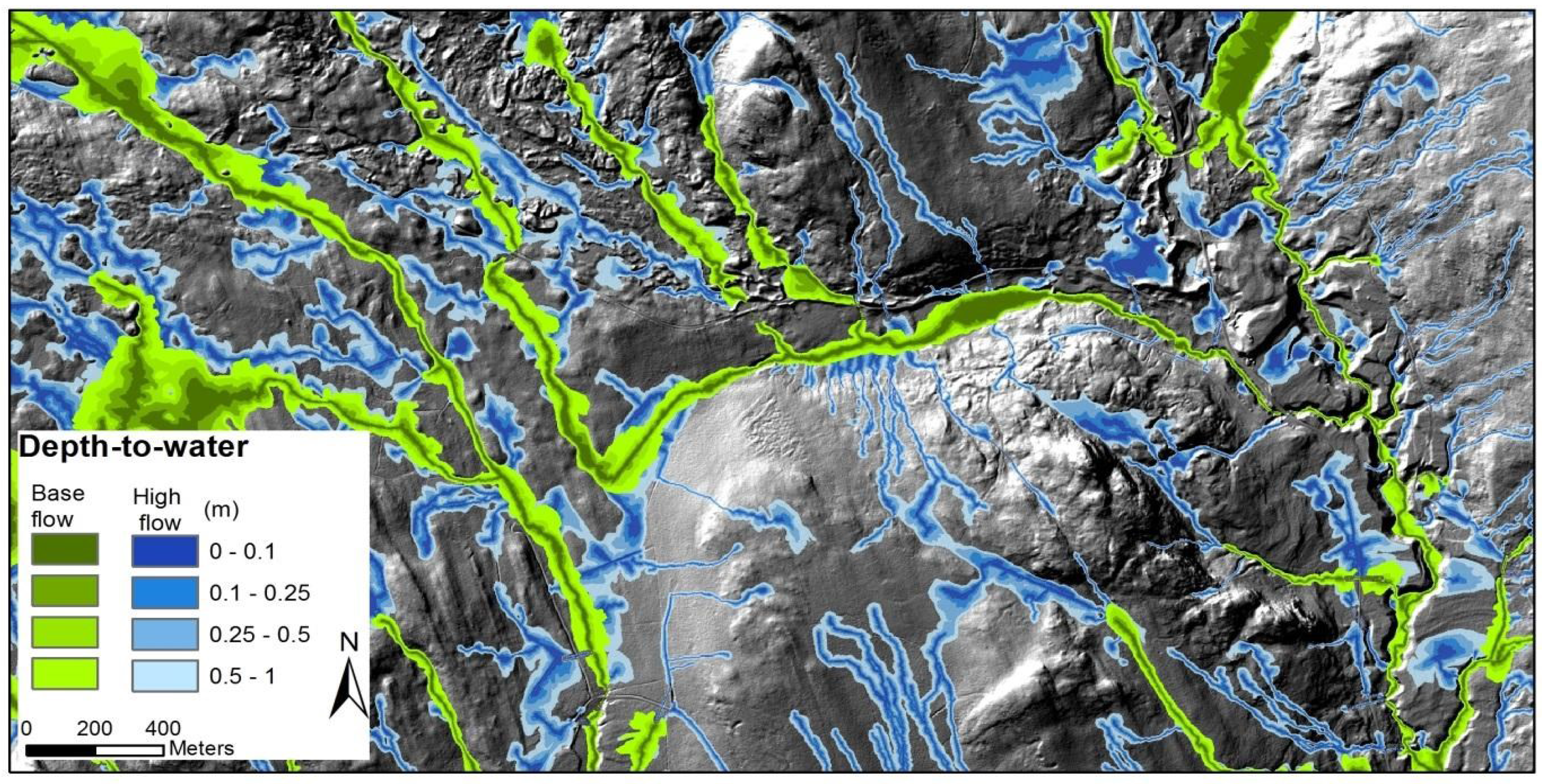
2.2. Wet Areas Mapping

The distribution of wet areas, the discharge areas was modelled throughout the landscape from the DEM. A discharge area is an area where groundwater emerges at the surface; an area where upward pressure or hydraulic head moves groundwater towards the surface. Ågren et al. [42] tested several methods of calculating wet areas from digital terrain indices and found that cartographic Depth-to-water index (DTW) was a robust method with high predictive power for soil wetness. The DTW index [43,44] is the least-cost elevation difference (in meters) to the nearest open water body (in our case the field-mapped stream network). The cells in the stream network were set to be 0. DTW was then determined for each of the resulting flow networks according to Equation (1).
[ D T W   ( m ) =   [ d z i d x i a ] x c ]
where dz/dx is the slope of a cell along the least-elevation path, i is a cell along the path, a is 1 when the path crosses the cell parallel to the cell boundaries and 1.414214 when it crosses diagonally; xc represents the grid cell size (m) [43].
The area of the landscape that was classified as a discharge area (DTW < 1 m) was calculated (Figure 5). In the lower lying part of the catchment there is a sedimentary area including patches of agriculture land, and large low-productive mires are common in the upper parts of the catchment. Because the focus of this study is on forest land, anything outside productive forest land (defined as land with a potential mean yield capacity of at least 1 m3 for total stem volume over bark per ha and year over one rotation period) was excluded from the calculations.

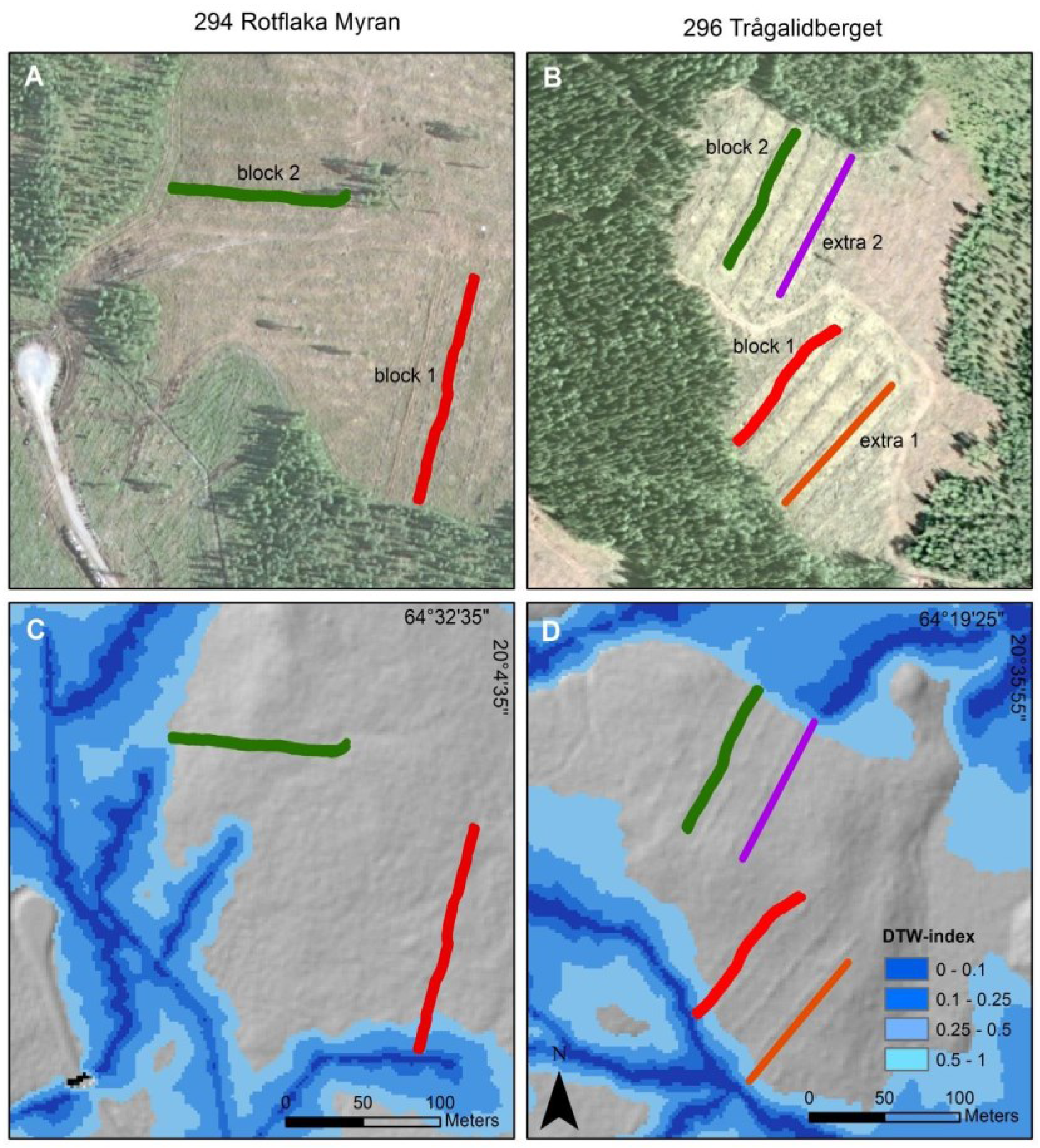
2.3. A Case Study: Rutting Caused by Forwarder Traffic in Relation to Generated DTW-Maps

Data from a study-plot experiment situated in Northern Sweden (Figure 6) on 64°32.5′ N, 20°4.3′ E and 64°19.4′ N, 20°35.5′ E were used to compare the results of the DTW-maps against field measurements of rutting. DTW-maps were generated for the study sites as described in Section 2.2 and compared with the rutting caused by repeated passes with a laden forwarder. The treatments, applied to study plots established along four harvested hillslopes, consisted of no forwarder traffic and forwarder traffic without soil protection, on logging residues and on logging mats, respectively. The study plots were clear-cut, without driving on the plots, about half a year and one and a half year, respectively, before applying the treatments. Here, we only present results from the treatment without soil protection (Figure 6 and Figure 7).
Figure 5. The black and white background map shows the sunlit elevation model of a subsection of the Krycklan catchment. Superimposed are the depth-to-water index maps which mark the wet areas along the stream network. Blue areas indicate wet areas during spring flood and green areas indicate areas that remain wet during baseflow. The darker colors (blue or green) indicate that the modelled groundwater level is closer to the soil surface and hence wetter.
Forests 06 02982 g005
The forwarder was a John Deere 1410D with eight wheels mounted on four axles. It was equipped with 700 mm wide tires and bogie tracks on both front and rear wheel pairs. The total weight (obtained from measurements) of the laden forwarder was approx. 35 Mg at site 294 Rotflaka Myran and 33 Mg at site 296 Trågalidberget. The forwarder drove up and down the harvested slopes two to three times, a total of four to six passes. Due to severe rutting, some passes had to be shortened at the downslope end. The rut depth from the original soil surface was measured with a ruler at 1 m interval along the study plots.

2.4. Expansion of Discharge Areas Following Final Felling

After final felling, the water balance changes because evapotranspiration is reduced after removal of the trees. This in turn leads to an increase in storage of water, i.e., increasing groundwater levels which in turn increase runoff but also expand the discharge area. Using Darcy’s law and Dupuit assumptions that the flow on each level is horizontal, the expansion of discharge area up along the hillside can be calculated. Site 294 Rotflaka Myran was used as an example because the till at 296 Trågalidberget was more heterogeneous.
Figure 6. Field experiment in northern Sweden, using study plots in a randomized block design, to study forwarder traffic on harvested slopes. (A,B) show the aerial photos of the study sites and the location of the wheel tracks in the study plots subjected to the treatment forwarder traffic without soil protection (red lines for the wheel tracks in block 1, green lines for block 2, and purple and orange lines for two additional plots which were not part of the original study); (C,D) show the sunlit elevation model (in greyscale) with a high flow DTW-index map superimposed (1 ha stream initiation). The location of the green baseflow DTW model as seen in Figure 5 is not visible in these areas, but starts just outside the displayed maps.
Forests 06 02982 g006
The saturated discharge area starts at a distance from the water divide where the recharge to the groundwater above equals the maximum possible groundwater discharge (when the groundwater reaches the soil surface). Mathematically,
[ R · x · w = K · t · w · d h d x ]
where:
  • R = recharge to the groundwater (m·s−1)
  • x = distance to the water divide (m)
  • w = width of the slope (m)
  • K = saturated hydraulic conductivity of the soil layer (m·s−1)
  • t = thickness of the soil layer (m)
  • d h d x = slope of the groundwater surface (assumed to be the same as the soil surface)
The K-value was calculated using SOILPAR 2.0, a program that estimates soil physical and hydrological parameters. The Puckett method [45] was selected and the K-value was calculated from the average particle size distribution of four soil samples sampled at 20 cm depth along the plots (Figure 6). We also calculated the K-value by solving the equation for K based on the following assumptions; The recharge to groundwater (R) on till soils in the study region is 375 mm·yr−1 [46]. x was measured to 175 m based on the distance from the top of the hill down to a mire below the plots that was defined as the border of the discharge area prior to felling. w was the same before and after final felling and can therefore be deleted on both sides of the equation. In till soils, hydraulic conductivity typically decreases more or less exponentially with depth. Here, we approximated that all lateral water movements along the slope occurred in the upper 1 m of the soil (t), which is a good approximation for many Fennoscandian till soils [47,48]. dh/dx was measured on the digital elevation model to 0.06 m·m−1. The expansion of the discharge area was calculated by solving the equation for x assuming that clear cutting the area increased the recharge to the groundwater by 200 mm·yr−1 [49]. Assuming that all of the recharge to groundwater becomes runoff, 200 mm·yr−1 seems to be a fair approximation since six catchments in Scandinavia showed increases in runoff, up to 10 years following clear-cut, by on average 193 mm·yr−1 (SD = 90) [50].
Figure 7. Rut depth in study plots subjected to repeated passes by a laden forwarder in the study-plot experiments (means for the left and right wheel tracks). The rut depth was not measured in case the mineral soil was unexposed in the track. The colors of the bars correspond to the plots in the map (Figure 6) and the error bars represents the standard deviation.
Forests 06 02982 g007

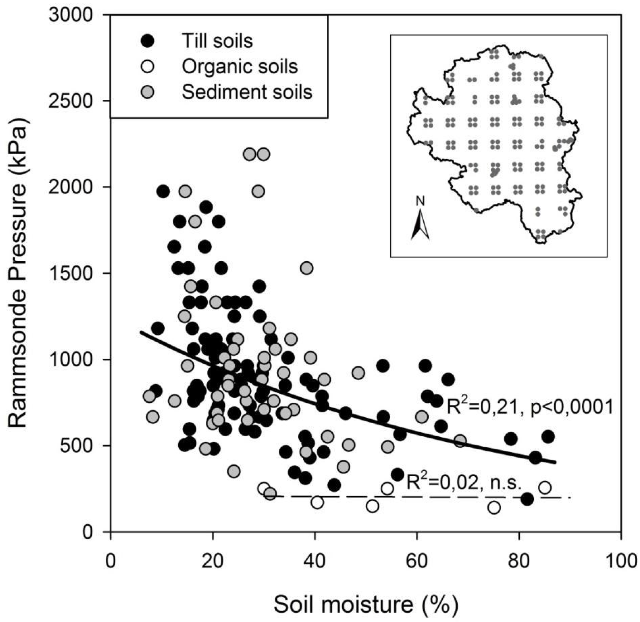
2.5. Measurements of Soil Bearing Capacity and Soil Moisture

Soil bearing capacity and soil moisture was measured at 160 locations in the Krycklan by Edlund [51]. The soil bearing capacity, here measured as Rammsonde Pressure (RP), was measured using a modified Swiss Rammsonde [52]. In short, a cone penetrometer sits mounted on a hollow shaft with a drop hammer mounted on top. The cone is placed on the soil and the penetration into the soil was measured after dropping the hammer 40 cm above the shaft five times. The RP was calculated according to [52]. The RP is the force per m2 needed to penetrate the probe in the soil. Soil moisture was measured with TDR technique using a ThetaProbe ML2x.

3. Results and Discussion

3.1. Spatial and Temporal Variability in Stream Drainage Network and Associated Wet Soils

In this study, we found that there was a large temporal variability in the drainage area needed before a stream head was found, i.e., in stream initiation threshold area. During the two snowmelt events (Q = 4.13 and 2.9 mm·day−1) the stream heads corresponded to threshold areas between 0.4 and 4.4 ha (Figure 2).
The re-inventory during the lowest base flow event showed that only three streams were still actively transporting water and the stream heads were found after 11.4–15.8 ha. The smallest stream initiation areas were often associated with ditches that were activated during times of high flow, while natural trickles occurred on top of the forest floor (Figure 1A,B). During baseflow, the trickles were associated with peat soil in small valley bottoms (Figure 1C) or in the main channels. The stream initiation threshold was inversely related to specific discharge (Figure 2). At times with high specific discharge (Q > 0.5 mm·day−1), the stream initiation threshold was approximately 2 ha (and 1 ha if the land was drained by ditches). During baseflow situations (Q < 0.5 mm·day−1), the stream initiation threshold increased rapidly to about 10–15 ha. Because of the larger variability during baseflow and the fact that the threshold changed rapidly with Q during baseflow situations (Figure 2), it is difficult to identify one threshold value representative of baseflow situations. The long term discharge records for the monitored site C7 (Svartberget) in the Krycklan Catchment, from 1981 and onwards [37], show that the specific discharge is below 0.5 mm·day−1 during 50% of the snow-free period (May–November). Hence, the stream network using the 2 ha flow initiation is active during 50% of the bare ground-period.
By varying the stream initiation threshold in the GIS calculations, the stream network during different flow conditions can be mapped (Figure 3). Figure 4 illustrates how the total length of the stream network changes with stream initiation threshold, which reflects changes with the hydrological situation. According to our calculations, the Krycklan stream network expands from 177 km during baseflow (using a conservative threshold of 10 ha which can be seen to represent a normal year) to 432 km during spring flood (using a conservative threshold of 2 ha) (Figure 3 and Figure 4).
Thus, on an annual basis, the length of the stream network at high-flow conditions is 2.4 times the length at baseflow conditions. On the national map of Sweden with the highest resolution, the Property map (1:12,500, Lantmäteriet, Gävle), the stream network in the study catchment is 102 km. Consequently, only 58% of the estimated 177 km perennial stream network was present on the Property map. When taking into consideration that the entire stream network (using 2 ha flow initiation) was active during 50% of the snow free-period, this corresponds to a situation where 76% of the stream network is lacking on the most detailed map (1: 12,500). These numbers are similar to the findings from a study conducted in the Chattooga River catchment in southern US [53], where 50%–75% of the perennial streams were identified on topographic maps, depending on scale (1:24,000 and 1:100,000). In the same study, only 14%–21% of the fully expanded stream network was mapped on topographic maps. The main explanation to this is that the current maps have been drawn from aerial photos where the smaller streams in the forest landscape are invisible under tree canopies. Obviously, if more than half of the streams are missing on the maps, this renders forestry planning with respect to surface water difficult.
The depth-to-water map illustrates how different stream networks can be used to model discharge areas during different flow situations. During low flow, 8% of the forest land was classified as being wet (following the DTW < 1) while during high flow the corresponding share was 31%. This number includes the mires which are integral parts of the forest landscape, but they are often low-productivity sites and are therefore often not subjected to forest management. Of the productive forest land (≥1 m3·ha−1·yr−1 for total stem volume over bark), the discharge area covered 5% and 25% during low and high flow, respectively. This illustrates the dynamics of forest hydrology and the challenges this poses in planning forestry activities for which the variability in trafficability needs to be taken into account. However, from the field survey of the stream heads, we can capture the expansion and shrinkage of the stream-network in a GIS-model and map the discharge areas during dry and wet conditions (Figure 5).
The map shows the modelled wet areas around the perennial stream network (green area, Figure 5) and the expansion during high flows (blue). Best management practices for riparian buffer zones vary throughout the world [21]. A general trend though is that, due to their large length in the landscape [34], small headwater streams receive less protection [29,54]. The new maps (as the map in Figure 5) can be used to create hydrologically adapted buffer zones as suggested by Kuglerova et al. [55,56] and improve protection for surface water quality by identifying wet areas where for instance off-road forestry traffic and fertilization should be avoided. The main advantages with these new maps are that: (1) the entire perennial stream network is present on the maps; (2) the maps can be made available on computers of forest machinery, thus, providing machine operators with detailed site information. Furthermore, areas sensitive to physical soil disturbance [57] can be identified, since the blue areas on the maps (Figure 5) indicate areas with high hydrological connectivity. Because of this connectivity, any exposed mineral soil in these areas is likely to be transported to the stream network at high-flow situations, increasing erosion and sediment transport in the draining stream with deleterious effects on downstream aquatic habitats [58]. By identifying areas that could be operated during dry conditions but should be avoided during wet conditions, more rutting and soil scarification can be avoided and one major concern for water quality due to forestry can be addressed. While field verification (using hydric soils, the hydrophytic vegetation or the presence of subsurface or surface water to detect the wet soils) is the most reliable way [53] to properly plan management of riparian forests, we propose that the time for this can be reduced by using DEM derived stream networks and associated wet soils. The maps can also be used in snowy conditions when the snow hinders field verifications and unfrozen wet soils underneath the snow can be sensitive for trafficking. To take into account temporal variability in the stream network, in operational forestry is a challenge for the future, but one that can be addressed with these kinds of LiDAR derived maps (Figure 5).

3.2. Soil Bearing Capacity as a Function of Soil Moisture and Soil Type

The DTW maps model the depth down to a supposed groundwater surface, from that it follows that the closer the groundwater level is to the ground surface the wetter the soil should be. However, for forest soil trafficking, it is not so much soil moisture per se that is of interest, but the effect the moisture has on the bearing capacity on the soil. A field study measuring soil bearing capacity in the Krycklan catchment using a modified Swiss Rammsonde [52] showed that there was a significant negative relationship between Rammsonde Pressure and soil moisture (Figure 8). The organic soils had the lowest bearing capacity with RPs less than 500 kPa, independent of the soil moisture. From a surface water protection perspective, this has implications as riparian soils both are wet (which decrease the bearing capacity of mineral soils) and it is common with formation of riparian peats along stream channels [59] due to elevated groundwater levels during much of the year. On dryer soils, ruts are shallow and are mainly formed by compaction of the soil, while on wetter soils rutting causes soil deformation and displacement [60]. This means that the soils along streams are more sensitive to deformation because of both high water content and higher organic content (Figure 8). The large variability in the scatterplot could partly be attributed to the fact that local soil bearing capacity of forest soils also depend on stoniness and root systems, which was observed during the field inventory (Edlund, [61]).
Figure 8. Rammsonde Pressure (RP) and soil moisture measured at 160 locations in the Krycklan Catchment (inset figure). Results are divided into mineral soils (grey and black dots) and organic soils (white dots). Modified from Edlund [52].
Forests 06 02982 g008

3.3. Expansion of Discharge Areas Following Final Felling

When tree stands are harvested the water balance changes, evapotranspiration is reduced until the tree cover has re-established and during this period water storage in soils and runoff increases [62,63]. This means that discharge areas expand uphill following final felling hence, ruts or other soil disturbances within this area may be connected to surface water and cause deleterious sediment transport. Predicting and mapping this expansion would give forestry planning a way to better manage the quality of surface waters. Using the K-value estimated from SOILPAR, the distance from the water divide to the discharge area changed from 1003 m to 654 m following clear-cutting, meaning that the discharge area would expand 349 m upslope following clear-cutting. When solving the equation for the K-value, the distance from the water divide to the discharge area changed from 175 m to 114 m following clear-cutting, meaning that the discharge area would expand 61 m upslope. This shows how sensitive the calculations of the expansions are to the K-value and how uncertain the K-values are. In our study, the K-value for the soil calculated from soil texture was 1.9 × 10⁻⁴ m·s−1, while the K-value by solving the equation for K was 3.3 × 10⁻⁵ m·s−1. Another investigation comparing different measurement techniques on a till soil gave K-values ranging from 5.7 × 10⁻⁶ to 1.9 × 10⁻² mm·s−1 [64]. This illustrates how K-values are notoriously difficult to measure and development of maps that can predict the expansion of the discharge areas with any kind of accuracy seems unlikely because of the (1) sensitivity of the calculations to the K-value; (2) large uncertainties in measured K-values; (3) general lack of K-values for different parts of the landscape and also (4) large spatial variation in K-values within till soils (the dominating quaternary deposits in northern boreal zone).
Despite this, we can still put these results in the perspective of the study-plot experiment. The expansion of the discharge area, based on the K-value measured at 20 cm depth, gave unreasonable numbers. K-values have been found to decrease with soil depth in Scandinavia [48,65,66,67,68] and elsewhere [69,70], and using a K-value from 20 cm depth (1.9 × 10⁻⁴ m·s−1) therefore overestimates the overall groundwater-flow in the slope.
The saturated hydraulic conductivity calculated by solving the equation for K (3.3 × 10⁻⁵ m·s−1) was close to measured values of saturated hydraulic conductivity in a soil profile in till at Gårdsjön, southern Sweden, where average K was 3 × 10⁻⁵ m·s−1 [66]. Based on this K-value, the discharge area would expand in the order of 60 m upslope following clear-cutting at Rotflaka Myran. In the rutting experiment ruts were formed up along the hillslope of roughly that order (Figure 7), indicating wet conditions of up to 100 m uphill.

3.4. Preventing Rutting

The soil bearing capacity at a given time and space is determined by several interacting factors like soil type, stoniness, root systems and weather situation in combination with the wetting up of soils following clear-cut [71,72,73]. The DTW maps for the study-plot experiment (Figure 6) predicted that only the area at the very bottom of the hillslopes acted as discharge areas. Yet, ruts (≥20 cm deep wheel tracks) were formed some 75–100 m uphill at 294 Rotflaka Myran (Figure 7), and 26–50 m at 296 Trågalidberget, indicating that the DTW maps cannot be used for predicting rutting. However, they can be used to identify the areas where rutting can lead to deleterious sediment transports in adjacent streams and ditches. Ruts in the grey areas on the map in Figure 5 pose a smaller risk for increased sediment transport than ruts in the blue and green areas where the connectivity to the stream is high, and the soils are wetter and richer in organic matter which makes them more susceptible to soil disturbance (Section 3.2). The DTW maps provide the foresters with information on where off-road traffic should be avoided or soil reinforcement must be made, for instance by applying slash or logging mats. Since logging residues constitutes a significant source for forest biofuel, we further suggest that the maps can be used to balance the use of slash for soil and surface water protection and bioenergy harvest. From a surface-water perspective aiming at protecting the near-stream zone from soil disturbance, harvest of slash can be conducted on the soils that are indicated to be dry on the DTW maps which in our case corresponded to 75% of the productive forest area (Figure 5). Note, however, that extra consideration to avoid soil disturbance might be needed also within the grey areas on the maps for example to protect cultural heritage or recreational values.
Apart from protecting the blue and green areas from soil disturbance, it would be useful to also include the area which temporarily will act as discharge area after final felling. However, today we find it difficult to use the DTW maps for predicting the expansion of the discharge areas following final felling, mainly due to the difficulty in finding or estimating accurate K-values for forest soils. The large variability in the length of the ruts at 296 Trågalidberget probably mirrors the variation in soil types within the site, and consequently the variation in K-values.

4. Conclusions

The field survey showed that there was a large temporal and spatial variability in the stream network. It is important to consider this variability when planning forestry operations. Wet area maps (DTW maps) using different flow initiation thresholds can be used to map discharge areas around stream networks for different flow situations representative of different seasons. Our calculations show that due to the lack of, and the poor quality of K-values, it is not possible today to model the expansion of discharge areas following clear-cutting. Thus, the DTW maps cannot be used to predict rutting in general but they can target those areas in need of most protection from a surface-water perspective. The maps can be used in forestry planning to: identify zones sensitive to traffic and soil disturbance, suggest site-specific forest buffer zones around the perennial stream network, and plan routes for the forestry machinery. We argue that the DTW map for the base-flow stream network (green in Figure 5) can be used to design hydrologically adapted forest buffer zones, variable in width, along perennial streams as suggested by Kuglerova [56]. We further argue that the area within the DTW maps for high-flow situations (Blue in Figure 5) can be used to indicate areas sensitive to soil disturbance, for instance, that caused by off-road forestry traffic and soil scarification. Thus, the transport of deleterious sediment to adjacent streams may be avoided.

Acknowledgments

This project was financed by the Swedish Energy Agency, Mistra’s Future Forest program, The Swedish Research Council Formas, Formas’ ForWater, Stiftelsen fonden för skogsvetenskaplig forskning, the Kempe foundation and VINNOVA.

Author Contributions

Anneli Ågren planned the field investigation in the Krycklan catchment, performed all GIS analysis and calculations, analyzed the data, reanalyzed the data from Edlund [51], and led the writing of the article. William Lidberg performed the field survey of the stream heads and contributed to the writing. Eva Ring lead the study-plot experiment at 294 Rotflaka Myran and 296 Trågalidberget and contributed to the writing.

Conflicts of Interest

The authors declare no conflict of interest.

References

  1. Egnell, G.; Laudon, H.; Rosvall, O. Perspectives on the Potential Contribution of Swedish Forests to Renewable Energy Targets in Europe. Forests 2011, 2, 578–589. [Google Scholar] [CrossRef]
  2. Stephenson, A.L.; FRS, D.J.M. Life Cycle Impacts of Biomass Electricity in 2020. Available online: https://www.gov.uk/government/uploads/system/uploads/attachment_data/file/336038/beac_report.pdf (accessed on 1 June 2015).
  3. Kreutzweiser, D.P.; Hazlett, P.W.; Gunn, J.M. Logging impacts on the biogeochemistry of boreal forest soils and nutrient export to aquatic systems: A review. Environ. Rev. 2008, 16, 157–179. [Google Scholar] [CrossRef]
  4. Laudon, H.; Tetzlaff, D.; Soulsby, C.; Carey, S.; Seibert, J.; Buttle, J.; Shanley, J.; McDonnell, J.J.; McGuire, K. Change in winter climate will affect dissolved organic carbon and water fluxes in mid-to-high latitude catchments. Hydrol. Process. 2013, 27, 700–709. [Google Scholar] [CrossRef]
  5. Naghdi, R.; Solgi, A. Effects of Skidder Passes and Slope on Soil Disturbance in Two Soil Water Contents. Croat. J. For. Eng. 2014, 35, 73–80. [Google Scholar]
  6. Frey, B.; Kremer, J.; Rudt, A.; Sciacca, S.; Matthies, D.; Luscher, P. Compaction of forest soils with heavy logging machinery affects soil bacterial community structure. Eur. J. Soil Biol. 2009, 45, 312–320. [Google Scholar] [CrossRef]
  7. Schnurr-Putz, S.; Baath, E.; Guggenberger, G.; Drake, H.L.; Kusel, K. Compaction of forest soil by logging machinery favours occurrence of prokaryotes. Fems Microbiol. Ecol. 2006, 58, 503–516. [Google Scholar] [CrossRef] [PubMed]
  8. Frey, B.; Kremer, J.; Rudt, A.; Sciacca, S.; Matthies, D.; Luscher, P. Heavy-Machinery Traffic Impacts Methane Emissions as Well as Methanogen Abundance and Community Structure in Oxic Forest Soils. Appl. Environ. Microbiol. 2011, 77, 6060–6068. [Google Scholar] [CrossRef] [PubMed]
  9. Teepe, R.; Brumme, R.; Beese, F.; Ludwig, B. Nitrous oxide emission and methane consumption following compaction of forest soils. Soil Sci. Soc. Am. J. 2004, 68, 605–611. [Google Scholar] [CrossRef]
  10. Schaffer, J.; Wilpert, K.V. In situ observation of root growth behind rhizotron windows—A pilot study. Allg. Forst Und Jagdztg. 2012, 183, 1–15. [Google Scholar]
  11. Curzon, M.T.; D’Amato, A.W.; Palik, B.J. Harvest residue removal and soil compaction impact forest productivity and recovery: Potential implications for bioenergy harvests. For. Ecol. Manag. 2014, 329, 99–107. [Google Scholar] [CrossRef]
  12. Kreutzweiser, D.P.; Capell, S.S. Fine sediment deposition in streams after selective forest harvesting without riparian buffers. Can. J. For. Res. 2001, 31, 2134–2142. [Google Scholar] [CrossRef]
  13. Sidle, R.C.; Ziegler, A.D.; Negishi, J.N.; Nik, A.R.; Siew, R.; Turkelboom, F. Erosion processes in steep terrain—Truths, myths, and uncertainties related to forest management in Southeast Asia. For. Ecol. Manag. 2006, 224, 199–225. [Google Scholar] [CrossRef]
  14. Prevost, M.; Plamondon, A.P.; Belleau, P. Effects of drainage of a forested peatland on water quality and quantity. J. Hydrol. 1999, 214, 130–143. [Google Scholar] [CrossRef]
  15. Lisle, T.E. Sediment Transport and Resulting Deposition in Spawning Gravels, North Coastal California. Water Resour. Res. 1989, 25, 1303–1319. [Google Scholar] [CrossRef]
  16. Soulsby, C.; Youngson, A.F.; Moir, H.J.; Malcolm, I.A. Fine sediment influence on salmonid spawning habitat in a lowland agricultural stream: a preliminary assessment. Sci. Total Environ. 2001, 265, 295–307. [Google Scholar] [CrossRef]
  17. Lemly, A.D. Modification of benthic insect communities in polluted streams: Combined effects of sedimentation and nutrient enrichment. Hydrobiologia 1982, 87, 229–245. [Google Scholar] [CrossRef]
  18. Munthe, J.; Hultberg, H. Mercury and Methylmercury in Runoff from a Forested Catchment—Concentrations, Fluxes, and Their Response to Manipulations. Water Air Soil Pollut. Focus 2004, 4, 607–618. [Google Scholar] [CrossRef]
  19. Gerasimov, Y.; Sokolov, A.; Fjeld, D. Improving Cut-to-length Operations Management in Russian Logging Companies Using a New Decision Support System. Balt. For. 2013, 19, 89–105. [Google Scholar]
  20. Hiesl, P.; Benjamin, J.G. Applicability of International Harvesting Equipment Productivity Studies in Maine, USA: A Literature Review. Forests 2013, 4, 898–921. [Google Scholar] [CrossRef]
  21. Broadmeadow, S.; Nisbet, T.R. The effects of riparian forest management on the freshwater environment: A literature review of best management practice. Hydrol. Earth Syst. Sci. 2004, 8, 286–305. [Google Scholar] [CrossRef]
  22. Gundersen, P.; Lauren, A.; Finer, L.; Ring, E.; Koivusalo, H.; Saetersdal, M.; Weslien, J.O.; Sigurdsson, B.D.; Hogbom, L.; Laine, J.; et al. Environmental Services Provided from Riparian Forests in the Nordic Countries. Ambio 2010, 39, 555–566. [Google Scholar] [CrossRef] [PubMed]
  23. Luke, S.H.; Luckai, N.J.; Burke, J.M.; Prepas, E.E. Riparian areas in the Canadian boreal forest and linkages with water quality in streams. Environ. Rev. 2007, 15, 79–97. [Google Scholar] [CrossRef]
  24. Vidon, P.; Allan, C.; Burns, D.; Duval, T.P.; Gurwick, N.; Inamdar, S.; Lowrance, R.; Okay, J.; Scott, D.; Sebestyen, S. Hot Spots and Hot Moments in Riparian Zones: Potential for Improved Water Quality Management. J. Am. Water Resour. Assoc. 2010, 46, 278–298. [Google Scholar] [CrossRef]
  25. Wilkerson, E.; Hagan, J.M.; Siegel, D.; Whitman, A.A. The effectiveness of different buffer widths for protecting headwater stream temperature in Maine. For. Sci. 2006, 52, 221–231. [Google Scholar]
  26. Blinn, C.R.; Kilgore, M.A. Riparian management practices—A summary of state guidelines. J. For. 2001, 99, 11–17. [Google Scholar]
  27. Lee, P.; Smyth, C.; Boutin, S. Quantitative review of riparian buffer width guidelines from Canada and the United States. J. Environ. Manag. 2004, 70, 165–180. [Google Scholar] [CrossRef]
  28. Sweeney, B.W.; Newbold, J.D. Streamside forest buffer width needed to protect stream water quality, habitat, and organisms: A literature review. J. Am. Water Resour. Assoc. 2014, 50, 560–584. [Google Scholar] [CrossRef]
  29. Richardson, J.S.; Naiman, R.J.; Bisson, P.A. How did fixed-width buffers become standard practice for protecting freshwaters and their riparian areas from forest harvest practices? Freshw. Sci. 2012, 31, 232–238. [Google Scholar] [CrossRef]
  30. Richardson, J.S.; Danehy, R.J. A synthesis of the ecology of headwater streams and their riparian zones in temperate forests. For. Sci. 2007, 53, 131–147. [Google Scholar]
  31. Mazor, R.D.; Stein, E.D.; Ode, P.R.; Schiff, K. Integrating intermittent streams into watershed assessments: Applicability of an index of biotic integrity. Freshw. Sci. 2014, 33, 459–474. [Google Scholar] [CrossRef]
  32. Bishop, K.; Buffam, I.; Erlandsson, M.; Folster, J.; Laudon, H.; Seibert, J.; Temnerud, J. Aqua Incognita: The unknown headwaters. Hydrol. Process. 2008, 22, 1239–1242. [Google Scholar] [CrossRef]
  33. Acuna, V.; Datry, T.; Marshall, J.; Barcelo, D.; Dahm, C.N.; Ginebreda, A.; McGregor, G.; Sabater, S.; Tockner, K.; Palmer, M.A. Why Should We Care About Temporary Waterways? Science 2014, 343, 1080–1081. [Google Scholar] [CrossRef] [PubMed]
  34. Blyth, K.; Rodda, J.C. Stream Length Study. Water Resour. Res. 1973, 9, 1454–1461. [Google Scholar] [CrossRef]
  35. Rummukainen, M.; Bergstrom, S.; Persson, G.; Rodhe, J.; Tjernstrom, M. The Swedish Regional Climate Modelling Programme, SWECLIM: A review. Ambio 2004, 33, 176–182. [Google Scholar] [CrossRef] [PubMed]
  36. Andreasson, J.; Bergstrom, S.; Carlsson, B.; Graham, L.P.; Lindstrom, G. Hydrological change—Climate change impact simulations for Sweden. Ambio 2004, 33, 228–234. [Google Scholar] [CrossRef] [PubMed]
  37. Laudon, H.; Taberman, I.; Ågren, A.; Futter, M.; Ottosson-Löfvenius, M.; Bishop, K. The Krycklan Catchment Study—A flagship infrastructure for hydrology, biogeochemistry, and climate research in the boreal landscape. Water Resour. Res. 2013, 49, 7154–7158. [Google Scholar] [CrossRef]
  38. Laudon, H.; Berggren, M.; Agren, A.; Buffam, I.; Bishop, K.; Grabs, T.; Jansson, M.; Kohler, S. Patterns and Dynamics of Dissolved Organic Carbon (DOC) in Boreal Streams: The Role of Processes, Connectivity, and Scaling. Ecosystems 2011, 14, 880–893. [Google Scholar] [CrossRef]
  39. Lindsay, J.B.; Dhun, K. Modelling surface drainage patterns in altered landscapes using LiDAR. Int. J. Geogr. Inf. Sci. 2015, 29, 397–411. [Google Scholar] [CrossRef]
  40. Jenson, S.K.; Domingue, J.O. Extracting Topographic Structure from Digital Elevation Data for Geographic Information-System Analysis. Photogramm. Eng. Remote Sens. 1988, 54, 1593–1600. [Google Scholar]
  41. Ocallaghan, J.F.; Mark, D.M. The Extraction of Drainage Networks from Digital Elevation Data. Comput. Vis. Graph. Image Process. 1984, 28, 323–344. [Google Scholar] [CrossRef]
  42. Ågren, A.M.; Lidberg, W.; Strömgren, M.; Ogilvie, J.; Arp, P.A. Evaluating digital terrain indices for soil wetness mapping—A Swedish case study. Hydrol. Earth Syst. Sci. 2014, 18, 1–12. [Google Scholar] [CrossRef]
  43. Murphy, P.N.C.; Ogilvie, J.; Arp, P. Topographic modelling of soil moisture conditions: A comparison and verification of two models. Eur. J. Soil Sci. 2009, 60, 94–109. [Google Scholar] [CrossRef]
  44. Murphy, P.N.C.; Ogilvie, J.; Meng, F.R.; White, B.; Bhatti, J.S.; Arp, P.A. Modelling and mapping topographic variations in forest soils at high resolution: A case study. Ecol. Model. 2011, 222, 2314–2332. [Google Scholar] [CrossRef]
  45. Puckett, W.E.; Dane, J.H.; Hajek, B.F. Physical and Mineralogical Data to Determine Soil Hydraulic-Properties. Soil Sci. Soc. Am. J. 1985, 49, 831–836. [Google Scholar] [CrossRef]
  46. Rodhe, A.; Lindström, G.; Rosberg, J.; Pers, C. Grundvattenbildning i svenska Typjordar - Översiktlig Beräkning med en Vattenbalansmodell; Report Series A2006; Institutionen för geovetenskaper, Uppsala Universitet: Uppsala, Sweden; p. 27. (In Swedish)
  47. Seibert, J.; Grabs, T.; Kohler, S.; Laudon, H.; Winterdahl, M.; Bishop, K. Linking soil- and stream-water chemistry based on a Riparian Flow-Concentration Integration Model. Hydrol. Earth Syst. Sci. 2009, 13, 2287–2297. [Google Scholar] [CrossRef] [Green Version]
  48. Bishop, K.; Seibert, J.; Nyberg, L.; Rodhe, A. Water storage in a till catchment. II: Implications of transmissivity feedback for flow paths and turnover times. Hydrol. Process. 2011, 25, 3950–3959. [Google Scholar] [CrossRef]
  49. Grip, H.; Rodhe, A. Vattnets väg från regn till bäck, 3rd ed.; Hallgren & Fallgren: Uppsala, Sweden, 1994. (In Swedish) [Google Scholar]
  50. Sorensen, R.; Ring, E.; Meili, M.; Hogbom, L.; Seibert, J.; Grabs, T.; Laudon, H.; Bishop, K. Forest Harvest Increases Runoff Most during Low Flows in Two Boreal Streams. Ambio 2009, 38, 357–363. [Google Scholar] [CrossRef] [PubMed]
  51. Edlund, J. Harvesting in the Boreal Forest on Soft Ground—Ways to Reduce Ground Damage. Ph. D. Thesis, Department of Forest Rescource Management, Swedish University of Agricultural Science, Arkiteketkopia, Umeå, 2012. [Google Scholar]
  52. Bodin, A. Development of a tracked vehicle to study the influence of vehicle parameters on tractive performance in soft terrain. J. Terramechanics 1999, 36, 167–181. [Google Scholar] [CrossRef]
  53. Hansen, W.F. Identifying stream types and management implications. For. Ecol. Manag. 2001, 143, 39–46. [Google Scholar] [CrossRef]
  54. Fries, C.; Carlsson, M.; Dahlin, B.; Lämås, T.; Sallnäs, O. A review of conceptual landscape planning models for multiobjective forestry in Sweden. Can. J. For. Res. 1998, 28, 159–167. [Google Scholar] [CrossRef]
  55. Kuglerová, L.; Jansson, R.; Ågren, A.; Laudon, H.; Malm-Renöfält, B. Groundwater discharge creates hotspots of riparian plant species richness in a boreal forest stream network. Ecology 2013, 95, 715–725. [Google Scholar] [CrossRef]
  56. Kuglerová, L.; Ågren, A.; Jansson, R.; Laudon, H. Towards optimizing riparian buffer zones: Ecological and biogeochemical implications for forest management. For. Ecol. Manag. 2014, 334, 74–84. [Google Scholar] [CrossRef]
  57. Miwa, M.; Aust, W.M.; Burger, J.A.; Patterson, S.C.; Carter, E.A. Wet-weather timber harvesting and site preparation effects on coastal plain sites: A review. South. J. Appl. For. 2004, 28, 137–151. [Google Scholar]
  58. Wood, P.J.; Armitage, P.D. Biological effects of fine sediment in the lotic environment. Environ. Manag. 1997, 21, 203–217. [Google Scholar] [CrossRef]
  59. Grabs, T.; Bishop, K.; Laudon, H.; Lyon, S.W.; Seibert, J. Riparian zone hydrology and soil water total organic carbon (TOC): Implications for spatial variability and upscaling of lateral riparian TOC exports. Biogeosciences 2012, 9, 3901–3916. [Google Scholar] [CrossRef] [Green Version]
  60. Williamson, J.R.; Neilsen, W.A. The influence of forest site on rate and extent of soil compaction and profile disturbance of skid trails during ground-based harvesting. Can. J. For. Res. Rev. Can. Rech. For. 2000, 30, 1196–1205. [Google Scholar] [CrossRef]
  61. Edlund, J.; (Department of Forest Resource and Management, Swedish University of Agricultural Science, Umeå, Sweden). Personal Communication, 2012.
  62. Lundin, L. Effects on hydrology and surface water chemistry of regeneration cuttings in peatland forests. Int. Peat J. 1999, 9, 118–126. [Google Scholar]
  63. Brown, A.E.; Zhang, L.; McMahon, T.A.; Western, A.W.; Vertessy, R.A. A review of paired catchment studies for determining changes in water yield resulting from alterations in vegetation. J. Hydrol. 2005, 310, 28–61. [Google Scholar] [CrossRef]
  64. Mohanty, B.P.; Kanwar, R.S.; Everts, C.J. Comparison of Saturated Hydraulic Conductivity Measurement Methods for a Glacial-Till Soil. Soil Sci. Soc. Am. J. 1994, 58, 672–677. [Google Scholar] [CrossRef]
  65. Bishop, K.H.; Grip, H.; Oneill, A. The Origins of Acid Runoff in a Hillslope During Storm Events. J. Hydrol. 1990, 116, 35–61. [Google Scholar] [CrossRef]
  66. Nyberg, L. Water-Flow Path Interactions with Soil Hydraulic-Properties in Till Soil at Gardsjon, Sweden. J. Hydrol. 1995, 170, 255–275. [Google Scholar] [CrossRef]
  67. Laudon, H.; Seibert, J.; Köhler, S.; Bishop, K. Hydrological flow paths during snowmelt: Congruence between hydrometric measurements and oxygen 18 in meltwater, soil water, and runoff. Water Resour. Res. 2004, 40, W03102. [Google Scholar] [CrossRef]
  68. Beldring, S. Runoff generating processes in boreal forest environments with glacial tills. Nord. Hydrol. 2002, 33, 347–372. [Google Scholar]
  69. Kendall, K.A.; Shanley, J.B.; McDonnell, J.J. A hydrometric and geochemical approach to test the transmissivity feedback hypothesis during snowmelt. J. Hydrol. 1999, 219, 188–205. [Google Scholar] [CrossRef]
  70. Soulsby, C.; Reynolds, B. Influence of Soil Hydrological Pathways on Stream Aluminum Chemistry at Llyn-Brianne, Mid-Wales. Environ. Pollut. 1993, 81, 51–60. [Google Scholar] [CrossRef]
  71. Uusitalo, J.; Ala-Ilomaki, J. The significance of above-ground biomass, moisture content and mechanical properties of peat layer on the bearing capacity of ditched pine bogs. Silva Fenn. 2013, 47. article ID 993. [Google Scholar] [CrossRef]
  72. Vega-Nieva, D.J.; Murphy, P.N.C.; Castonguay, M.; Ogilvie, J.; Arp, P.A. A modular terrain model for daily variations in machine-specific forest soil trafficability. Can. J. Soil Sci. 2009, 89, 93–109. [Google Scholar] [CrossRef]
  73. Saarilahti, M. Soil interaction model. Available online: http://ethesis.helsinki.fi/julkaisut/maa/mvaro/publications/31/soilinte.pdf (accessed on 1 June 2015).

