Abstract
The use of optical remote sensing data for savanna vegetation structure mapping is hindered by sparse and heterogeneous distribution of vegetation canopy, leading to near-similar spectral signatures among lifeforms. An additional challenge to optical sensors is the high cloud cover and unpredictable weather conditions. Longwave microwave data, with its low sensitivity to clouds addresses some of these problems, but many space borne studies are still limited by low quality structural reference data. Terrestrial laser scanning (TLS) derived canopy cover and height metrics can improve aboveground biomass (AGB) prediction at both plot and landscape level. To date, few studies have explored the strength of TLS for vegetation structural mapping, and particularly few focusing on savannas. In this study, we evaluate the potential of high resolution TLS-derived canopy cover and height metrics to estimate plot-level aboveground biomass, and to extrapolate to a landscape-wide biomass estimation using multi-temporal L-band Synthetic Aperture Radar (SAR) within a 9 km2 area savanna in Kruger National Park (KNP). We inventoried 42 field plots in the wet season and computed AGB for each plot using site-specific allometry. Canopy cover, canopy height, and their product were regressed with plot-level AGB over the TLS-footprint, while SAR backscatter was used to model dry season biomass for the years 2007, 2008, 2009, and 2010 for the study area. The results from model validation showed a significant linear relationship between TLS-derived predictors with field biomass, p < 0.05 and adjusted R2 ranging between 0.56 for SAR to 0.93 for the TLS-derived canopy cover and height. Log-transformed AGB yielded lower errors with TLS metrics compared with non-transformed AGB. An assessment of the backscatter based on root mean square error (RMSE) showed better AGB prediction with cross-polarized (RMSE = 6.6 t/ha) as opposed to co-polarized data (RMSE = 6.7 t/ha), attributed to volume scattering of woody vegetation along river valleys and streams. The AGB change analysis showed 32 ha (3.5%) of the 900 ha experienced AGB loses above an average of 5 t/ha per annum, which can mainly be attributed to the falling of trees by mega herbivores such as elephants. The study concludes that SAR data, especially L-band SAR, can be used in the detection of small changes in savanna vegetation over time.
1. Introduction
Vegetation structure components such as above- and below-ground biomass, woody cover, tree height, basal volume, among others help with carbon stock estimation. According to the International Panel on Climate Change (IPCC) [1], aboveground biomass (AGB) constitutes “all living biomass above the soil including the stem, stump, branches, bark, seeds and foliage.” Valuation of these structural variables assists with the assessment of fuelwood consumption, relied upon by some 80% of sub-Saharan Africa, in addition to their ecological roles. Anthropogenic induced deforestation and natural forest degradation has led to the release of some 1–2 billion tons of carbon into the atmosphere, accounting for approximately 15%–20% of the global greenhouse gas (GHG) emissions [2]. By quantifying AGB through forest inventories, it is possible to understand the changes in the carbon pool and productivity of tropical forests [3,4]. Reliable AGB reporting is dependent on accurate field inventory, with regular updates, which is usually unavailable in most developing countries. Reliable allometric equations for AGB estimation in this region are few or poorly documented. This is partly attributed to the tedious work involved in the harvesting and weighing of tree species within an ecosystem, with large financial and time costs [5,6]. Hence, most allometric equations do not take into consideration the differences in tree species associated with variations in ecological regions. Allometric models are developed based on relationships between biomass and tree characteristics such as height and basal diameter [7]. Such relationships are therefore prone to errors associated with models used in their development [5,8]. Forest impenetrability, and time and financial constraints, have led to localized field inventories with few tree species [9], which are not representative over large areas [3,10]. Remotely sensed data are more suitable for biomass assessments over wider spatial coverages. However, the associated errors, mainly emanating from sampling procedures and errors associated with the allometric models, need to be taken into consideration. Until 2005, most allometries considered only the relationship between biomass, plant diameter, and wood specific density [5,6,8], leaving out the height variable. Examples of such allometries are presented in [6] where a linear relationship between AGB and log-transformed trees with D >33 cm in Kruger National Park (KNP) was derived, with 16% and 12% errors for woody and leaf biomass, respectively.
Many studies have developed empirical models to assess vegetation spectral response to biomass, with results indicating significant relationships between the two. Studies by [3] attributed these relationships to seasonal variations in phenological conditions, seen in visible and infrared bands of optical remote sensing datasets. Airborne laser scanners (ALS), light detection and ranging (Lidar) [11,12], and terrestrial laser scanners (TLS) can solve the problems associated with cloud contamination in imagery. Combining spectral reflectance with three-dimensional (3-D) capability facilitates canopy height estimations such as those shown in [13] where Geosciences Laser Altimeter (GLAS) Lidar onboard ICESat was combined with Shuttle Radar Topographic Mission (SRTM) to estimate forest heights in Brazil. Similar studies by [14] found a linear relationship between Lidar derived canopy cover and height metrics with AGB. Error identification and correction in AGB estimation is a major problem, and averaging canopy metrics at the plot scale is a major source of error in Lidar to field data correlation [15]. The potential of TLS in vegetation structural mapping are covered in [16,17,18,19]. Despite being a relatively new field, TLS allows a rapid acquisition of 3-D data with various applications [20,21,22,23]. Similar to Lidar, TLS represents a non-destructive method of obtaining biomass estimates, however, unlike Lidar, which covers large areas, TLS data capture is restricted to only a few meters [24,25]. Given its ability to acquire data on the ground, it can be used for validation of other remote sensing datasets [17,19]. However, a large number of point clouds are generated which would require sophisticated hardware and software for processing the data [26,27,28]. New methodological workflows like those adopted by [19] are able to extract individual trees from TLS point clouds by splitting trees into individual cylinders.
Additional three-dimensional feature data can be acquired remotely by microwave sensors. Synthetic Aperture Radar (SAR) employs active all weather sensors operated by sending a microwave radiation to targets and detecting the intensity of radiation scattered back to the sensor by the target (backscatter, σ0). The σ0 is a function of the incident angle θ, frequency, and polarization and is affected by the dielectric properties of the target and the surface geometry [29]. The wavelength (λ), relative to the size of the scatterer affects interactions between the two. Longer wavelengths are more relevant in the detection of vegetation geometry due to their penetrative effects, resulting in volume scattering [30,31]. The wavelength interaction with canopy elements results in diffuse scattering, hence more energy returning to the sensor [32]. SAR systems with longer wavelengths like L-band sensors penetrate into the canopy [29,33]. Cross-polarized measurements (HV or VH) work better than co-polarized (HH or VV) in correlating σ0 to AGB since the former accounts for canopy as opposed to ground components. By using dualpol SAR (both HH, HV), Mitchard et al. [30] found a relationship between AGB and σ0. Additional studies by [34,35] combined SAR and Lidar to improve AGB models by eliminating the bias that can occur from too many large trees. By using different polarizations of SAR with Landsat Enhanced Thematic Mapper (ETM) data, Wijaya et al. [36] developed empirical models to estimate how forest parameters responded to σ0 in Sumatra, while [37] assessed the relationship between dualpol σ0 and AGB using models after [38]. Relevant studies by [39] utilized multi-temporal and dual-pol SAR in assessing structural components of the vegetation within KNP. The capability of L-band SAR backscatter intensity in quantifying small-scale forest degradation in the Miombo woodlands of Mozambique over a three-year period was demonstrated in [32].
The present study, combining field inventory, high resolution TLS data, and L-band SAR data each with varying spatio-temporal resolutions, assesses (i) the use of sub-canopy data to estimate biomass at plot-level and the use of remote sensing datasets to upscale to the landscape level; and (ii) the potential of L-band SAR in biomass change detection within a savanna ecosystem. The current study is carried out within a Lowveld savanna. We established 42 field plots from which we inventoried tree height and basal diameter, and which we later used to compute plot-level aboveground biomass based on an allometric model specific to the study area. A TLS survey that was carried out in the same area provided vegetation canopy variables—canopy height and cover that were regressed with plot-derived AGB to generate a reference biomass for SAR biomass estimation for the study area. With multi-temporal SAR, we were able to assess biomass changes within the study area over a four-year period between 2007 and 2010. The study assessed the errors and accuracies associated with the models used.
2. Materials and Methods
2.1. Study Area
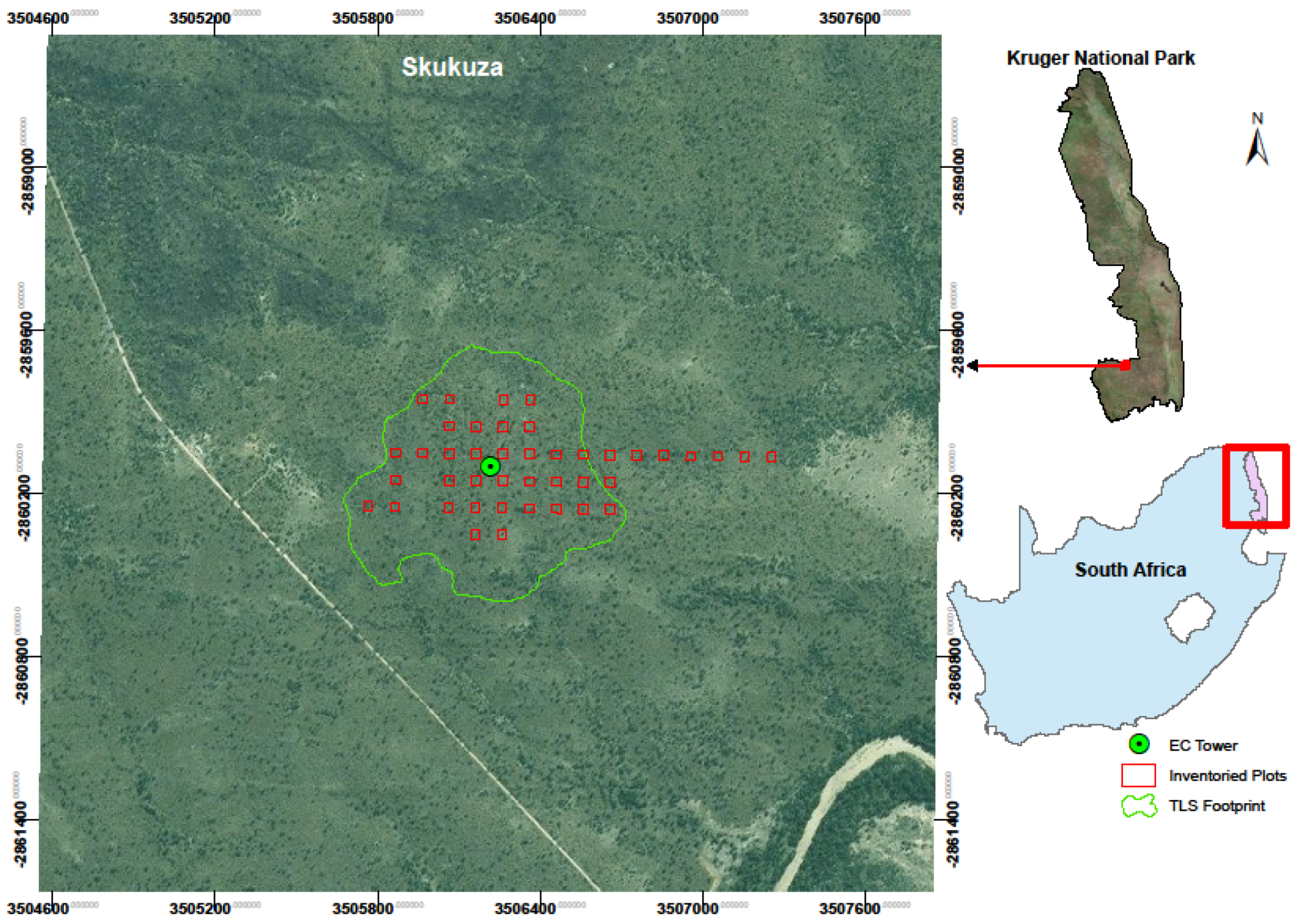
The study was conducted in the vicinity of the Skukuza Flux Tower located in the southern part of Kruger National Park (KNP) (Figure 1) about 13 km southwest of Skukuza in the N’waswitshaka catchment. The current study was done under the framework of the Adaptive Resilience of Southern African Ecosystems (ARS AfricaE) project. ARS AfricaE is implemented around eddy covariance flux towers to assess biogeochemical interactions and their significance to the resilience of the savanna biome to climate change [40]. The foregoing study was restricted to nine square kilometres around Skukuza Flux tower site. The flux tower (25.0197° S, 31.4969° E) was established in early 2000 to study carbon, water, and energy dynamics of semi-arid African savannas, as part of the South African Regional Science Initiative (SAFARI 2000) experiment to understand the interactions between the atmosphere and the land surface in southern Africa [41]. The landscape around the flux tower is typically undulating at an altitude ranging between 355 and 378 m above sea level (a.s.l.) [41,42,43], with Sabie River forming the major drainage system. The site is situated within broad- and fine-leafed savanna biome, an ecosystem covering 32% of South Africa. The dominant tree species here are Combretum sp. and Acacia sp. and the soil type is sandy clay loam Arenosol [42]. The area receives a mean annual precipitation of 547 mm and the mean annual temperature is 21.9 °C. The area is underlain by granite and gneiss and characterized by very distinctive catena sequence of soils from the crest to the valley bottom [14], with reddish or yellowish brown sand, grey hydromorphic sand, and clay (seasonal waterlogged band of soils).
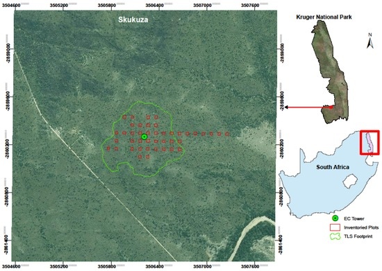
Figure 1.
Imagery showing location of the study site in Skukuza, inventoried plots and terrestrial laser scanner (TLS) footprint. The study is centered around the Skukuza eddy covariance tower (EC Tower) as shown in the map. (Imagery source: Google Earth/Digital Globe).
The characteristic biome is subtropical savanna, where the cover is not discrete but rather characterized by a mixture of growth forms, primarily grasses, shrubs, and trees. Small patches and gradual transition between open and closed vegetation cover are typical features of these landscapes [44,45,46,47,48,49,50,51,52]. Such characterization has caused problems in not only differentiating between the grass, shrub, and tree vegetation cover, but also in making the use of spectral information from passive remote sensing a difficult challenge given the inherent complexities in its structure. There is high pressure exerted by population increases and the need for people to derive their livelihoods from this ecosystem. There has been a spike in the amount of poaching in Kruger National Park, particularly in recent years, and this constitutes one example of the effects humans have on this supposed “closed” environment. The significance of poaching does have an effect on the savanna ecosystem stability, particularly the poaching of macro-herbivores, which will finally be manifested in vegetation.
2.2. Summary on Methodology
The main objectives of this study were to upscale sub-canopy field data to assess landscape biomass using both optical and microwave datasets, and to use time series L-band SAR data to detect biomass changes over a small area within a savanna. Figure 2 shows a simplified methodology adopted in this study. We estimated AGB for the study area in three stages. First, we computed reference AGB from the field inventory, and then used it to predict AGB based on three TLS-derived canopy height metrics—canopy height, canopy cover, and their product as used by [14]; secondly, we derived AGB from L-band SAR backscatter intensities with TLS-derived AGB in the first stage as reference data. The final stage involved the use of the multi-temporal and dual polarization L-band SAR data, which was acquired during the dry season and processed after methodologies adopted from [31,39,41] to estimate the change in biomass over a four-year period between 2007 to 2010.
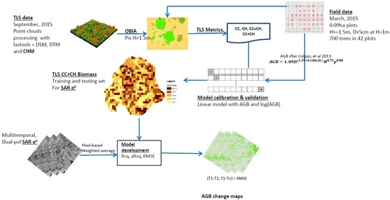
Figure 2.
A simplified methodology adopted in modelling aboveground woody biomass for this study. (The acronyms used in the flowchart are: DSM = digital surface model, DTM = digital terrain model, CHM = canopy height model, OBIA = object-based image analysis, Pix = pixel, H = tree height, D = diameter, Rsq = R-squared, RMSE = root mean square error).
2.3. Data Acquisition and Processing
2.3.1. Field Inventory Data
A detailed field inventory around the flux tower was carried out in March 2015. A total of 42 field-sampling plots, each measuring 30 m × 30 m were established around the tower. The location of the centre of each plot was recorded using Trimble eTrex handheld Global Positioning System (GPS). Within each plot, tree heights and basal stem diameters from stems greater than 5 cm thick were measured at 1 m from the ground and recorded. For tree heights, Nikon Forestry Pro laser rangefinder hypsometer was used to measure heights of trees taller than 1 m within the plots. The hypsometer uses a three-point height measurement function (trigonometry) by first calculating the horizontal distance, then capturing two other points to create an angle which it uses to accurately calculate vertical height. For basal diameter, a diameter-at-breast-height (DBH) tape was used to measure the basal diameter at 1 m height. In this study, a tree and a stem are loosely defined as single- or multi-stemmed individuals from the same rootstock and all branches from a particular point on the ground, respectively [14,15,53]. In cases where a tree had multiple stems, individual stems were measured, summed up and assigned to a single tree. In total 237 trees were inventoried during the field campaign.
2.3.2. Terrestrial Laser Scanner (TLS) Canopy Height Model (CHM)
TLS data was acquired for the study area over a 51.8 ha footprint around the flux tower in September 2015 using a RIEGL VZ-1000. The instrument uses a near infrared laser beam and is suitable for forestry research. The system provides a measurement range of up to 1400 m with 5 mm repeatability [54] (Table 1). Thirty scans were acquired around the flux tower at 300 kHz (limiting the range to 450 m) with an angular resolution of 0.015 degrees. Reference points determined by Real-Time Kinematic Global Navigation Satellite System (RTK-GNSS) measurements [55] were used to georeference the scans to the WGS84 ellipsoid. RiSCAN PRO software (provided by RIEGL) was used for the co-registration of the scans and point cloud generation. The point clouds were an octree data structure with a mean point density and spacing of 286.27 points/m2 and 0.05 m, respectively. To produce the pit-free CHM, the point clouds were processed using LAStools rapidlasso GmbH [56], following methodology used by [57] and substituting the platform from airborne to non-airborne to adapt the process to TLS data.

Table 1.
Riegl VZ-1000 specification (source: Riegl, 2015 [54]).
For the ease of manageability, we divided the point clouds into 250 MB large tiles with a 25 m buffer. ‘lasground.exe’ was used to extract bare-earth by classifying ground and non-ground points. All z-values above 0.1 m were dropped. We further used ‘lasthin.exe’ to simulate the diameter of the laser beam at 135 mm in 450 m distance from the scan position [58]. To replicate each point eight times in a discrete circle, we used a radius of 0.075 m around every input point, and then increased the spatial resolution of the point clouds two-fold to 0.03 m. Noise and unclassified points were filtered from ground points. Whereas we would expect pits within TLS data, similar to Lidar data, we still have height variations within forest stands and so we account for these by computing CHM at different height thresholds [57,59]. We therefore adopted the American Society of Photogrammetry and Remote Sensing (ASPRS) classification of Lidar point clouds by computing CHM for every class [60] as <0.5 m (bare + understory), 0.5–<2 m (low vegetation), 2–<5 m (medium vegetation), and ≥5 m (high vegetation). Following this sequence, we derived six CHMs. The consecutive 5 m interval heights help in improving the original morphological structure of tree crowns. According to [41], the average tree height within the study area is 9.1 m, weighed by tree basal area and so, apart from the flux tower and riverine vegetation which stand at about 21 m and above 21 m, respectively, most trees are below 20 m in height (Figure 3). The final step involved triangulating the four CHM height thresholds (bare + understory, low vegetation, medium vegetation, and high vegetation) using ‘blast2dem.exe’ to create a pit-free CHM as a GeoTiff by merging all the tiles. We used a kill size of 0.18 in triangulating Triangulated Irregular Networks (TINs), a value that is three times the step size (point resolution = 0.06 m). This would ensure that only triangles three times larger than the resolution were used for CHM generation. Figure 3a–c shows the resultant digital surface model (DSM), digital terrain model (DTM), and CHM.
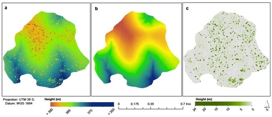
Figure 3.
TLS-derived (a) digital surface model; (b) digital terrain model; and (c) canopy height model.
2.3.3. LOS PALSAR L-Band Data
The Japan Aerospace Agency (JAXA) launched Phased Array L-band Synthetic Aperture Radar (PALSAR), on board Advanced Land Observation Satellite (ALOS) in 2006. PALSAR is a day and night all-weather land observation satellite, and is an active microwave sensor using L-band technology to achieve this capability. ALOS acquires data in both fine beam single (FBS) and fine beam dual (FBD) polarimetric modes with a range resolution of between 0 and 60 degrees. This study used four scenes with dual (HH-HV) polarizations for dry season since TLS data was captured during the dry season. Additionally, backscatter works well in the dry season due to low canopy and soil moisture [39,61]. Table 2 shows the specifications of L-band SAR datasets used in this study. ALOS PALSAR datasets were processed after [37]. GAMMA Remote Sensing and Consulting AG Modular SAR Processor (MSP) was used in SAR data preprocessing [62]. The datasets were acquired as level 1.1 single look complexes (SLC) with original radar geometry (range, Rg × azimuth, Az) of 9.37 m × 3.2, respectively, hence the first processing procedure was to apply multi-looking (ML) in order to derive backscatter intensity values. A sensor specific calibration factor of −115 dB was used to radiometrically calibrate the ML images. The backscatter images were then geocoded using a 20 m digital elevation model (DEM) by first generating the positional look-up table for each pixel in the SAR Range-Doppler and DEM geometry [37]. This was followed by simulation of SAR intensity from DEM to map geometry and a further transformation to SAR geometry. The final geocoding procedure involved the co-registration of real and simulated SAR in SAR geometry, and transformation of SAR Range-Doppler to map geometry.

Table 2.
Characteristics of the L-band Advanced Land Observation Satellite (ALOS) Phased Array L-band Synthetic Aperture Radar (PALSAR) used in the study. The datasets were acquired in Full Beam Dual (FBD) modes with Horizontal-Horizontal and Horizontal-Vertical (HH-HV) wave polarizations during dry seasons (DRY) between the years 2007 and 2010. T = Track, F = Frame. (source: JAXA).
To investigate speckle noise in the SAR data, we calculated the equivalent number of looks (ENL) by dividing the mean square backscatter intensity by variance (e.g., ENL = mean2/variance) after studies by [63]. The ENL was derived using a theoretical approach based on the nominal number of looks and the signal to noise ratio (SNR) according to Equation (1) due to heterogeneity of the study area.
where Nr and Naz are the number of range and azimuth looks, respectively. An increase in the ENL significantly reduces speckle noise in the multi-looked SAR data [39]. Accordingly, Argenti et al. [64] suggested that no filtering should be attempted on heterogeneous (point targets) areas. This is applicable to the current study area, and so the authors did not carry out noise filtering. Topographic normalization was then applied to the backscatter intensity images [65,66]. The final resultant geocoded and terrain corrected backscatter SAR images had a ground resolution of 12.5 m.
2.4. Aboveground Biomass (AGB) Modeling
2.4.1. Field Derived Biomass
We computed field-based aboveground biomass (AGB) in three steps. First, height (H) and basal diameter (D) of each tree was used to compute AGB at tree level in kilogram (kg) using Colgan allometry [15], as per Equation (2). This allometric equation was preferred because there exists no species specific allometry derived for this region of KNP, or for many of the individual species found in the site. The Colgan allometry used in this study was derived from destructive tree samples located outside of the park, within a Colophosperum mopane dominated savanna north of the study site. Many of the tree species sampled are commonly found in KNP, with a recommendation on a mean wood specific gravity of 0.9 [15].
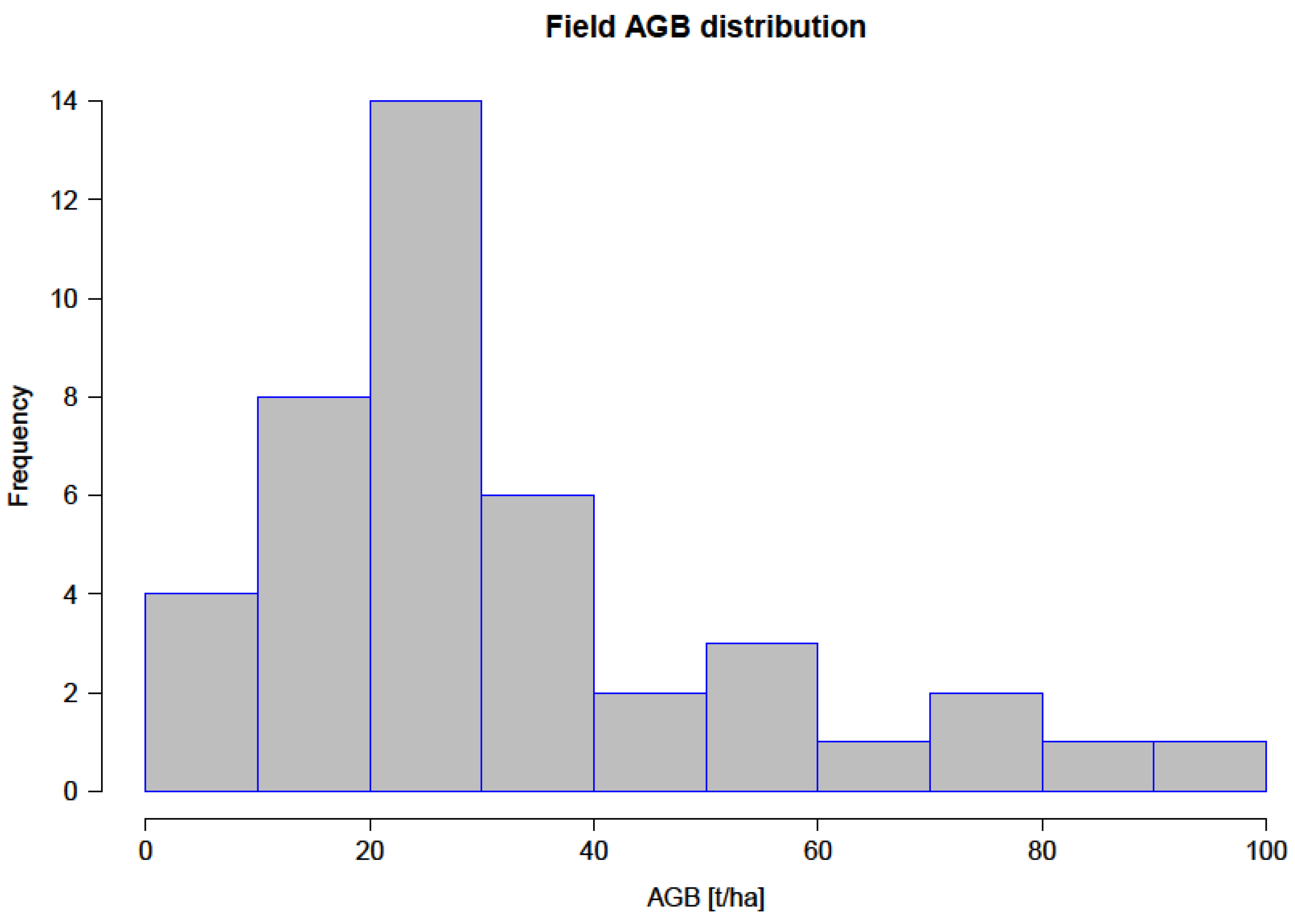
Second, all individual tree biomass within each plot was summed up, resulting in AGB in kg per plot. Biomass is usually expressed per unit area and so the final biomass was reported in metric tons per hectare (t/ha) after conversion based on the plot size of 0.09 ha. Table 3 gives a summary of the results from inventoried variables, while Figure 4 shows field biomass distribution within the study area, in t/ha.

Table 3.
Summary statistics of the inventoried trees. DBH = diameter at breast height; AGB = aboveground biomass.
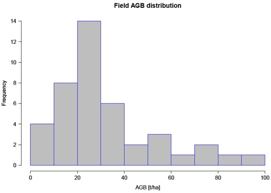
Figure 4.
Aboveground woody biomass distribution from field inventory data.
2.4.2. TLS CHM-Derived Biomass
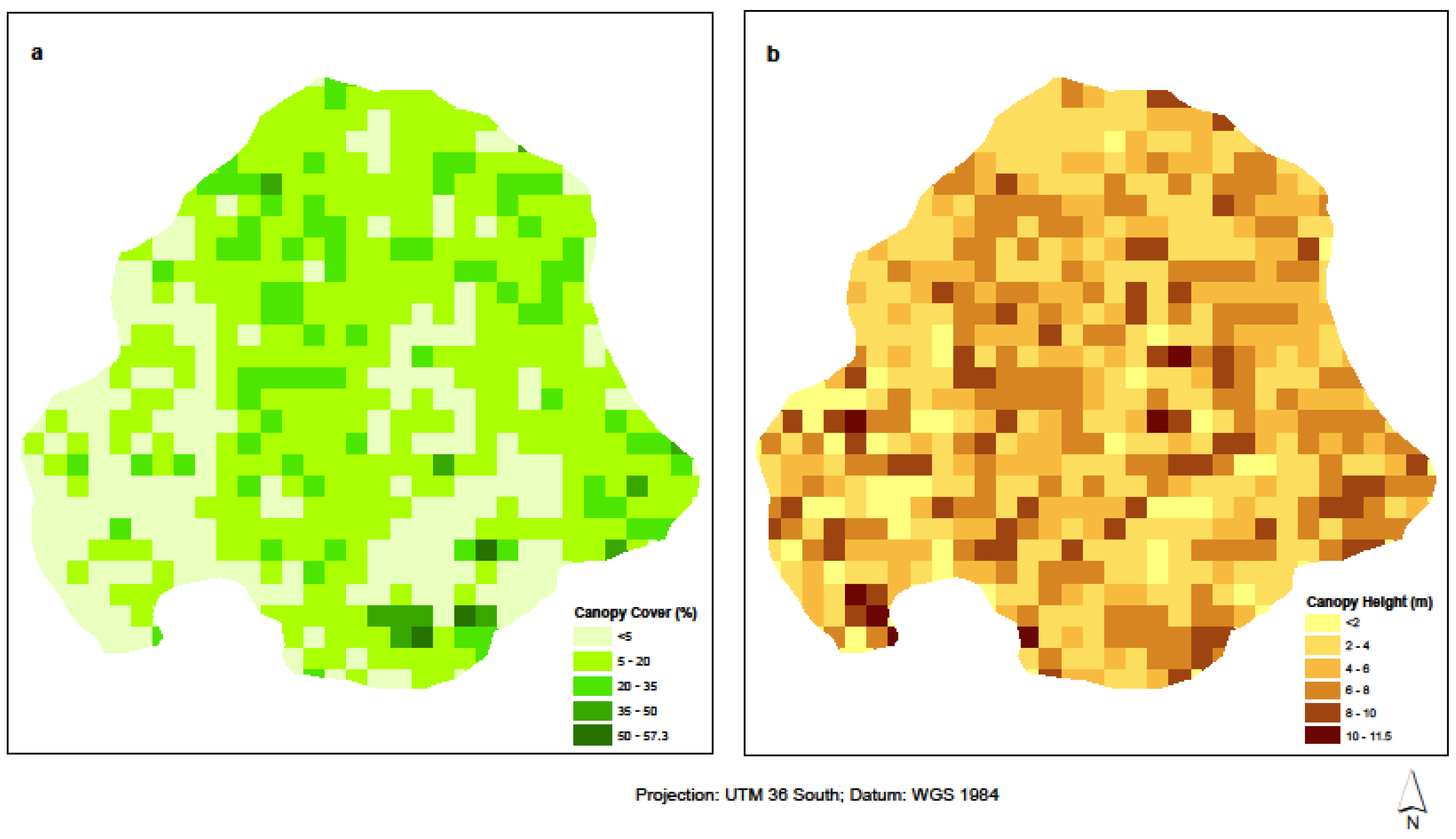
We used the field data to model AGB based on TLS metrics. The 6 cm TLS-derived canopy height model (CHM) was used in Trimble’s eCognition 8.9 [67] to delineate individual tree canopy cover and height. Pixel-based chessboard segmentation at a scale of 1 m resolution was performed on the CHM, with field plots as a thematic layer. Out of the 42 inventoried plots, only 33 plots fell within the TLS footprint, and so these were used as reference data in deriving AGB from TLS canopy metrics. A height threshold of 1 m was used to delineate pixels for canopy cover and canopy height, based on field inventory where only trees with heights >1 m were inventoried. This height ensured only woody vegetation contributed to biomass for the study area. Canopy cover (CC) was computed as the area of the plot with pixels having height >1 m, as a proportion of the entire plot, expressed in percentage. Canopy height on the other hand, is defined as the mean height of pixels with H >1 m per plot. Equations (3) and (4) show simplified formulas used to derive the two metrics, as adopted from [14]. An additional CHM metric was computed as the product of CC and CH (Figure 5a,b below), forming the third biomass predictor variable, CC × CH.
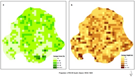
Figure 5.
(a) Percentage canopy cover and (b) canopy height for Skukuza flux tower site.
We assessed the predictive performance of each predictor on the field AGB to select the best amongst the three metrics. A linear regression model was used to predict biomass over the TLS footprint, using field computed AGB. We used 60% of the field AGB dataset for regression model calibration, and the remaining 40% for validation of the resulting predictions. To assess the linearity, we looked at the model performance in terms of the resultant root mean square error (RMSE) and bias (Equations (5) and (6)) from correlating the TLS metrics with both log (AGB) and normal AGB values [68]. To assess error distribution with AGB, we computed residuals (Equation (7)) as the difference between observed and predicted AGB for every TLS metrics.
The predictors were also fitted against the logarithm of AGB and the resultant residuals from both the field biomass and log-normal biomass were used to select the appropriate model for deriving AGB from TLS data. Studies by [6,15] both propose modelling the logarithm of field AGB, because DBH has a stronger linear relationship with log(AGB).
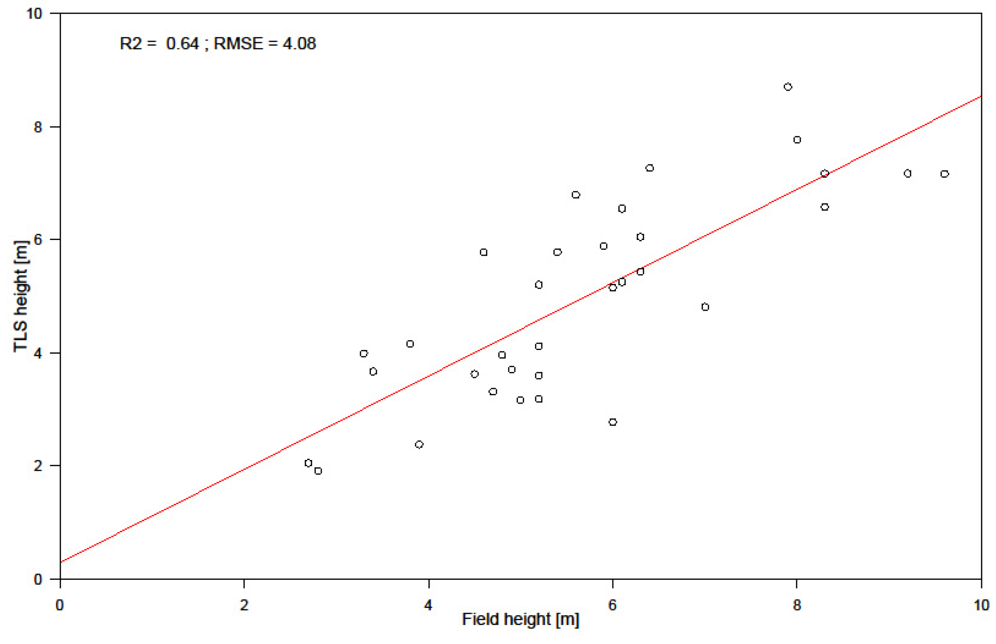
We did a comparison between the field measured height and the TLS-derived canopy height to assess the level of accuracy. Figure 6 shows the relationship between field measured height and the TLS-derived canopy height. The results show accuracy in field height measurement reducing with increasing height, with higher heights showing overestimation by the laser rangefinder.
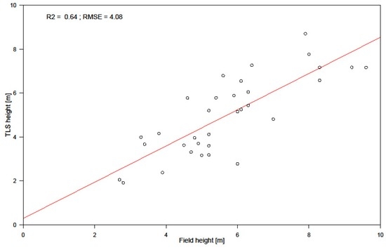
Figure 6.
Validation results of field measured height and TLS canopy height.
2.4.3. Estimating Aboveground Biomass from SAR
To compute AGB from L-band SAR, we used a weighted average of TLS AGB (AGBtls), due to the difference in resolution between the reference TLS-derived AGB (30 m) and the L-band SAR backscatter intensity (12.5 m) datasets. We assessed the contribution of field biomass to the intersecting 12.5 m SAR σ0 pixels by computing the area of pixels within each 30 m by 30 m field plots in order to get a weighted area, Wa. The AGB per intersecting object (AGBnew) was computed as the product of AGBtls and Wa. Chessboard segmentation was performed in eCognition with a scale of 1 (12.5 m), and the resultant pixels were intersected with AGBtls. We assessed SAR σ0 AGB based on polarizations (HH and HV), the years under investigation (2007–2010), and a combination of both using random forest and linear regression algorithms for polarimetric and yearly AGB estimations, respectively. Breiman et al. and Breiman [69,70] proposed random forest (RF) as ensemble learning for regression and classification trees, with successive trees not dependent on earlier trees (bootstrapping). In bagging, the best predictors are randomly chosen to split the tree, making RF a robust classifier against overfitting [71]. A script for this analysis was written in R statistical package. The analysis involved identification of the raster pixels within each reference AGB polygons. This was run on all the pixels within all four SAR backscatter raster grids.
2.4.4. Aboveground Biomass Change Analysis
Three image difference analyses were performed in ENVI, ArcGIS, and R statistical package. We assessed relative AGB changes per pixel for each of the three change combinations: 2007 to 2008, 2008 to 2009, and 2009 to 2010 for the study area. To decide whether a change was significant, we used R statistical package to reclassify both SAR backscatter predicted AGB and AGB change rasters at 5 t/ha intervals because the resultant SAR predictions had standard deviations less than 5 t/ha. We then overlaid the predicted biomass with a 2014 land cover map of the study area [72]. This allowed us to assess possible effects of such change on land cover.
3. Results
3.1. Field Biomass
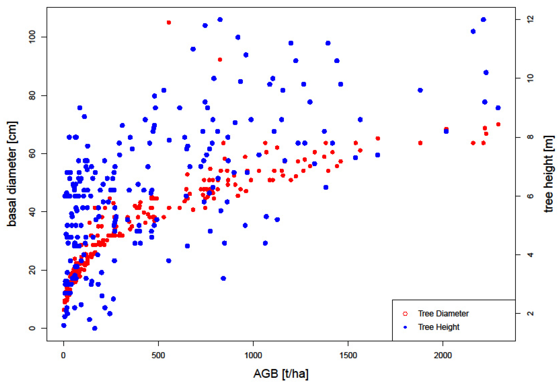
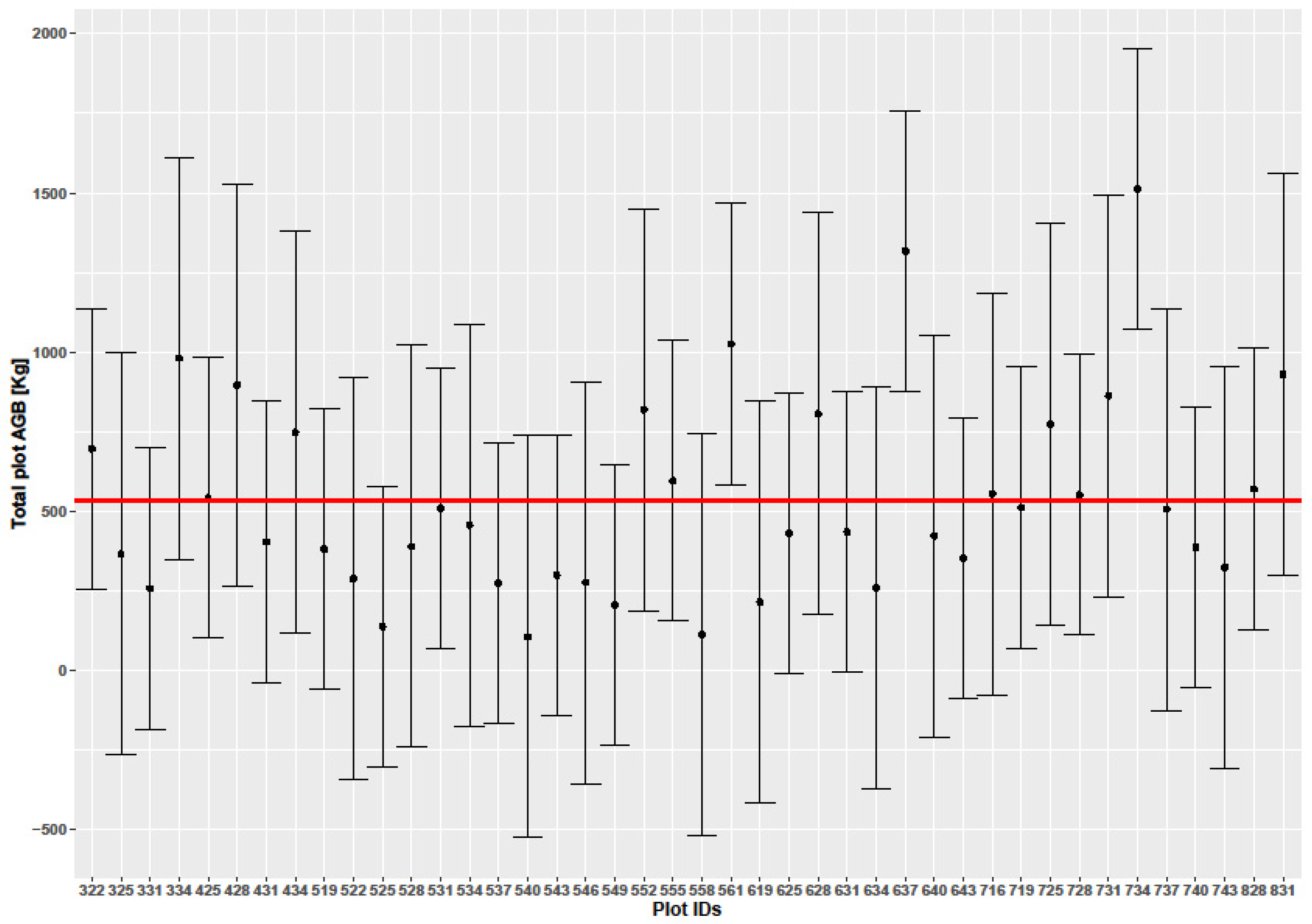
Figure 7 shows the distribution of field biomass per tree as computed from field inventory data. The mean AGB within the inventoried plots was 31.9 ± 21.3 t/ha, with the plot with the lowest biomass yielding 3.1 t/ha and the plot with the maximum biomass yielding 94.3 t/ha, consistent with similar studies carried out around Kruger National Park [6,15,53]. The trees within the inventoried plots had D ranging between 6.4 to 105 cm, and H of between 1.5 (inventory targeted trees with H > 1 m) to 12 m, with mean of 35 cm and 6.2 m for D and H, respectively. Most inventoried trees contributed biomass (median biomass) ranging between 20 and 30 t/ha, as can be seen from the field biomass distribution in Figure 4. Results from the 237 inventoried trees show variability with regards to AGB across the plots (Figure 8), with a total woody biomass of 120,414 kg. The mean AGB for all inventoried trees in the entire study site was 508.1 kg. The observed mean (± error margin) from all the 42 plots was estimated at 535.9 ± 95.1 kg (95% confidence interval: 441 to 631) as shown in Figure 8. Two plots (Id No. 322 and 716) recorded higher biomass values, with a total of three plots having 95% confidence intervals falling outside the overall mean biomass (31.9 t/ha) of the inventoried trees. From the plot in Figure 7, it is evident that D has a larger impact on the estimation of AGB than H.
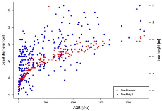
Figure 7.
Tree height, diameter, and the resultant AGB per inventoried tree within the study area.
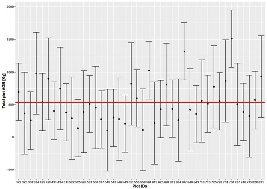
Figure 8.
Biomass estimates for each of the 42 sampled plots in kg. The red line shows the mean AGB in kg while the bars are 95% confidence intervals for AGB. Each plot is 0.09 ha in size.
3.2. Biomass Prediction Models
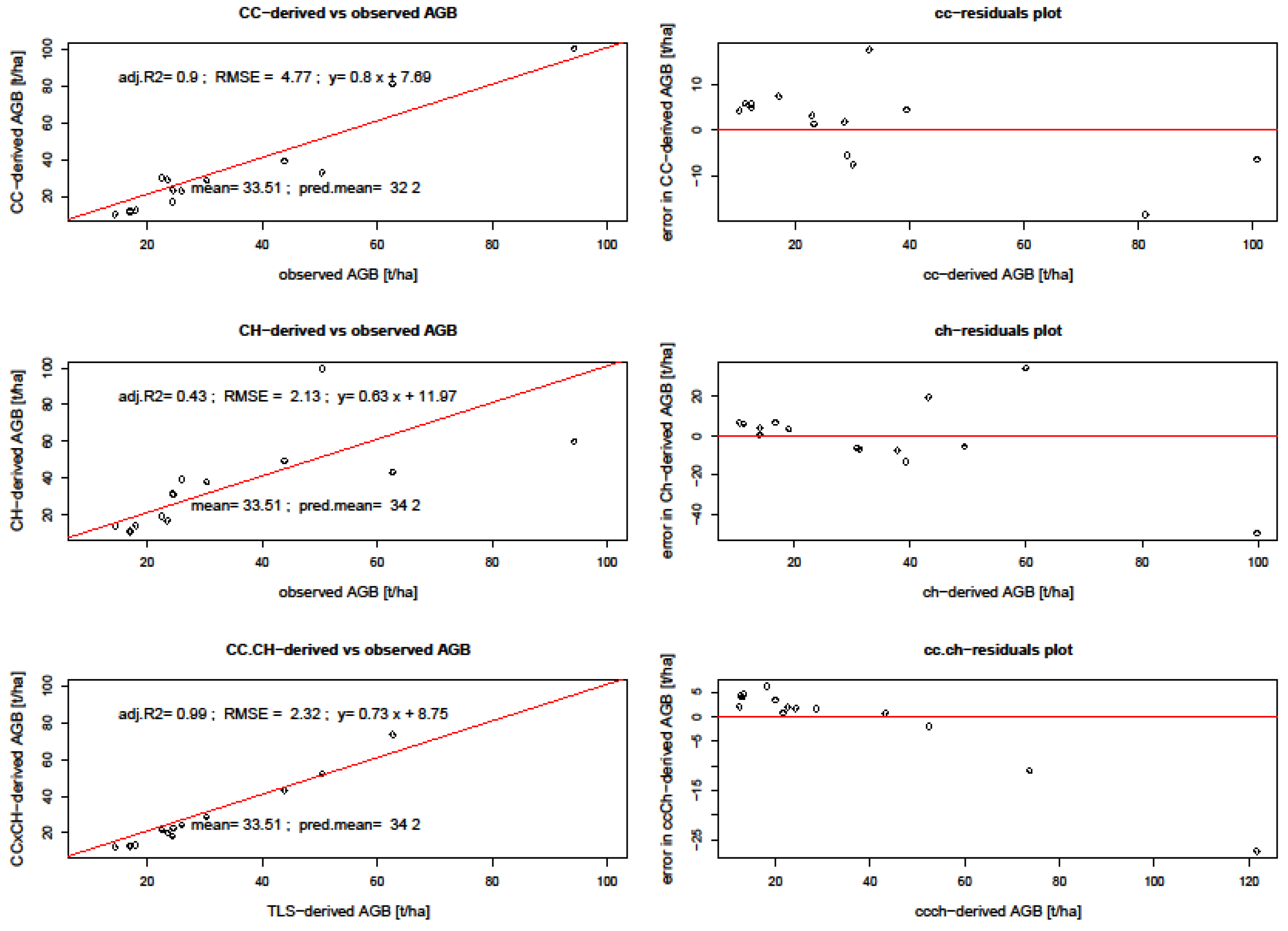
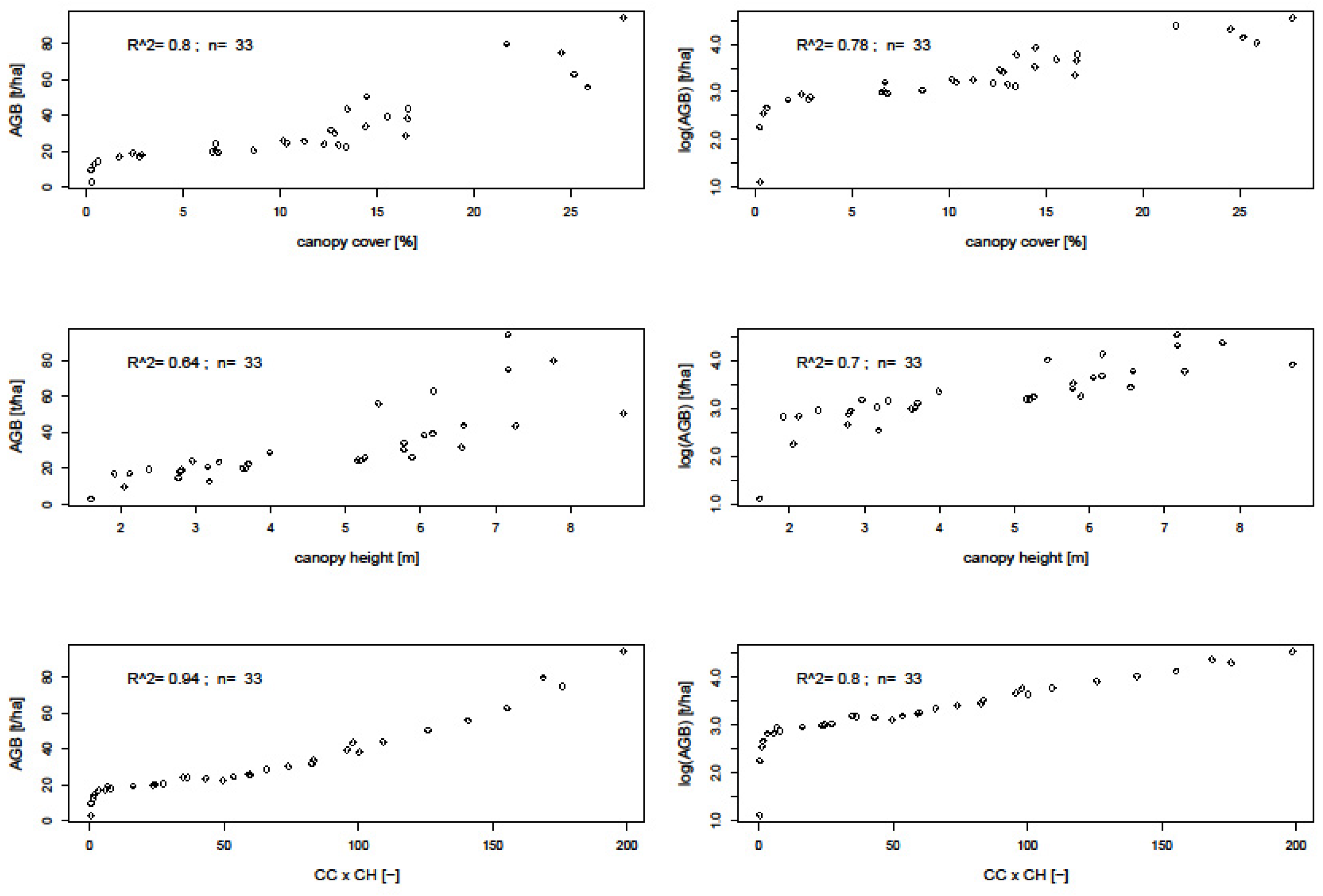
Table 4 summarizes field AGB performance to TLS-derived metrics and L-band SAR backscatter intensity performance to TLS-derived AGB (Figure 9). As expected, biomass values showed correlation with all the TLS metrics and L-band backscatter. Of the three TLS metrics, a product of canopy cover and canopy height performed better than the individual metrics, CC or CH, with the latter two resulting in root mean square errors (RMSE) of 4.77 t/ha and 2.13 t/ha, respectively [14]. From these results, it is evident that variance increases with increasing AGB. Studies by [6] propose log transformation of biomass to stabilize variance in order to achieve homoscedasticity. We therefore correlated the TLS metrics with both non-transformed and log-transformed plot biomass values (Figure 10) and further assessed the resultant errors from SAR backscatter prediction from the product of the two metrics.

Table 4.
TLS and microwave AGB predictor variables and associated error and coefficient of determination (R2).
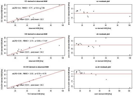
Figure 9.
Regression and residual plots between TLS metrics derived AGB and field. CC denotes canopy cover, CH denotes canopy height, and RMSE denotes root mean square error.
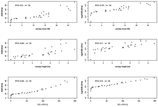
Figure 10.
Correlation between TLS canopy cover height metrics and AGB and log (AGB).
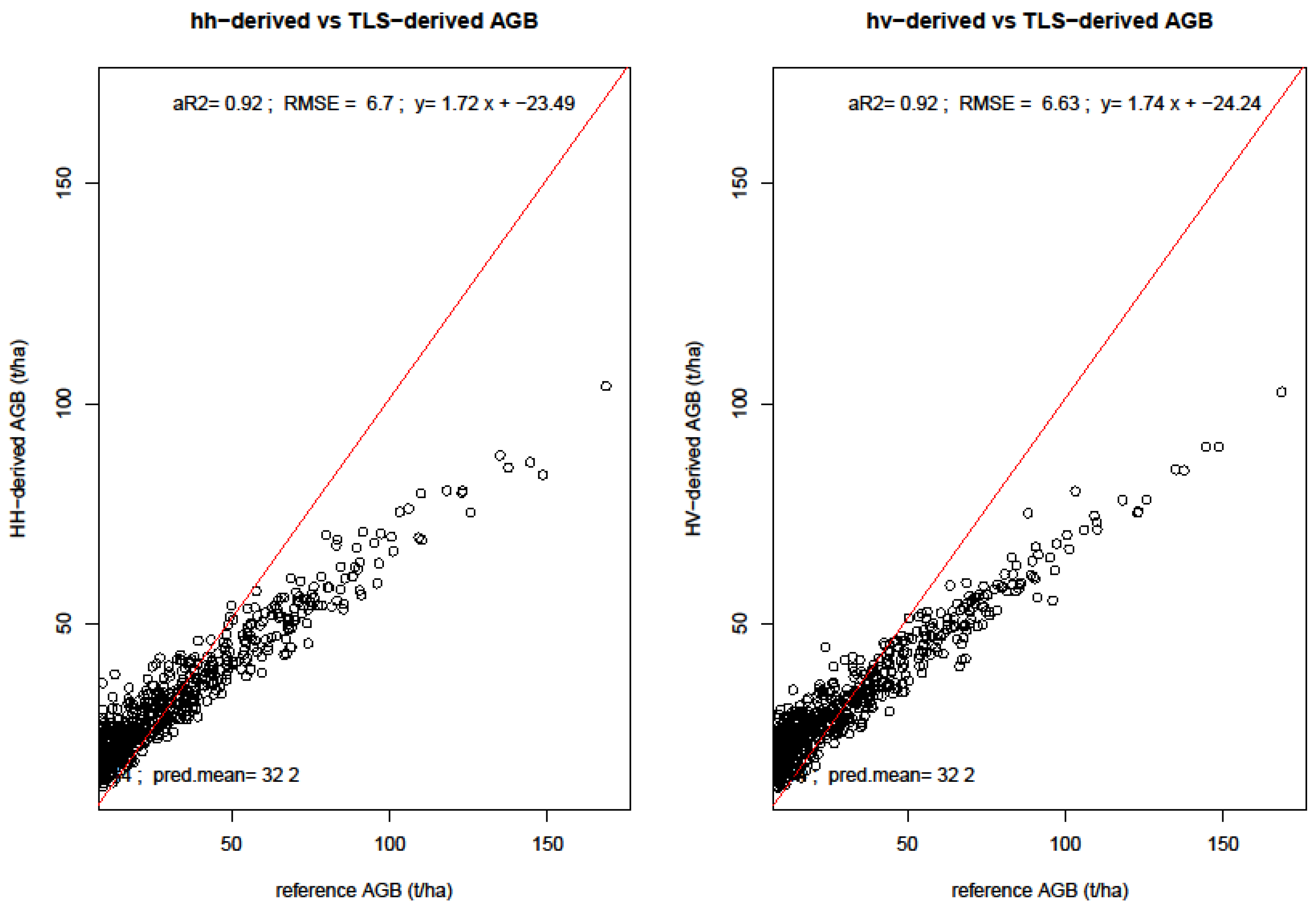
TLS-derived biomass had RMSE lower than 5 t/ha. The error obtained from predicting AGB using TLS metrics as reference is higher (6.7–6.6 t/ha for HH and HV, respectively) than that derived from field inventoried biomass values (2.1–4.8 t/ha). This is due to additional error which results from predicting the reference data (TLS-derived AGB) instead of field biomass. This was the case because the field data points derived from 33 field plots were few, and so the TLS-predicted AGB provided more data points necessary for landscape-wide AGB estimation. There is biomass underestimation by the SAR backscatter variables, as can be seen by both low mean biomass and the negative bias estimates. SAR backscatter-derived AGB had a mean of 32.2, which is lower than those from TLS metrics.
All AGB predictors yielded mean biomass ranging between 19.7 ± 5.2 t/ha for the 2010 SAR backscatter-based prediction, to 34.2 ± 30.78 t/ha for the product of the TLS cover and height prediction. All these values are within the range typical of biomass within the Lowveld savanna as presented by previous studies in this ecosystem. Noticeable is the high biomass values along the riverbanks due to riverine vegetation, and along the streamline. This can be explained by the fact that these areas store water that can be used by the trees after the end of the rainy season. The spatial distribution of trees in the study area has shown concentration of woody vegetation along the river valley, as attributed to fertile soil deposits from upland areas [73]. Further, Scholtz et al. and Baldeck et al. [74,75] cited soil catenal formations and associated soil and hydrological characteristics as major influences on landscape-scale vegetation structure and compositional variability.
3.3. Radar Sensitivity to Biomass
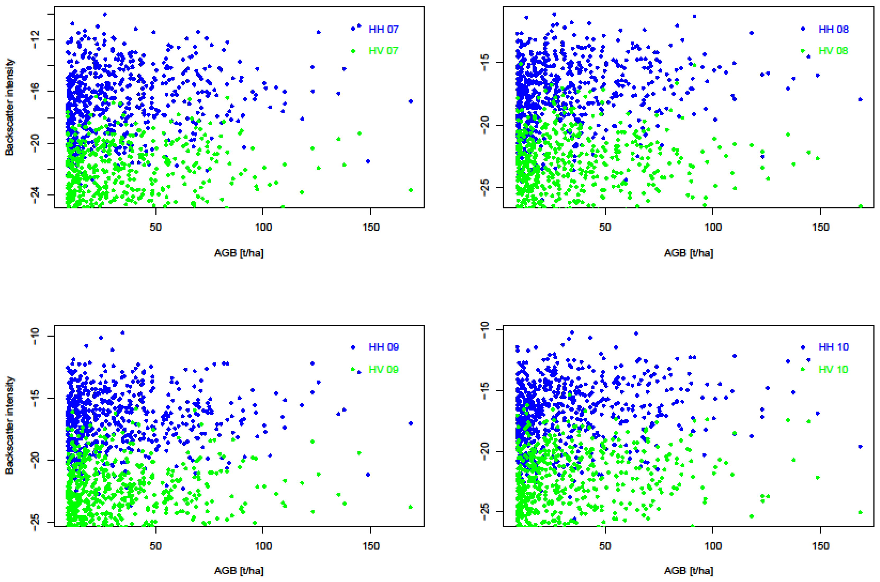
We evaluated the sensitivity of SAR backscatter to AGB in two ways. First, we looked at individual backscatter intensity, and then the SAR backscatter-derived biomass. Figure 11 shows both polarizations and their response to aboveground biomass over the four years. HV polarizations have lower backscatter values ranging between −30 dB to −15 dB, whereas HH polarizations have higher backscatter values from around −22 dB to −12 dB. The graphs show AGB detectability up to around 100 t/ha AGB, after which there are sparse or no backscatter points. This means that it might not be possible to accurately use SAR backscatter intensities in detecting AGB > 100 t/ha. From Table 4, the HV has a lower RMSE of 6.6 t/ha as opposed to the RMSE from HH polarization which had 6.7 t/ha.
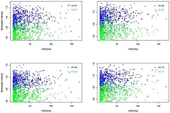
Figure 11.
Correlation between Synthetic Aperture Radar (SAR) backscatter intensities (HH and HV) and TLS-derived reference aboveground biomass for the years 2007–2010.
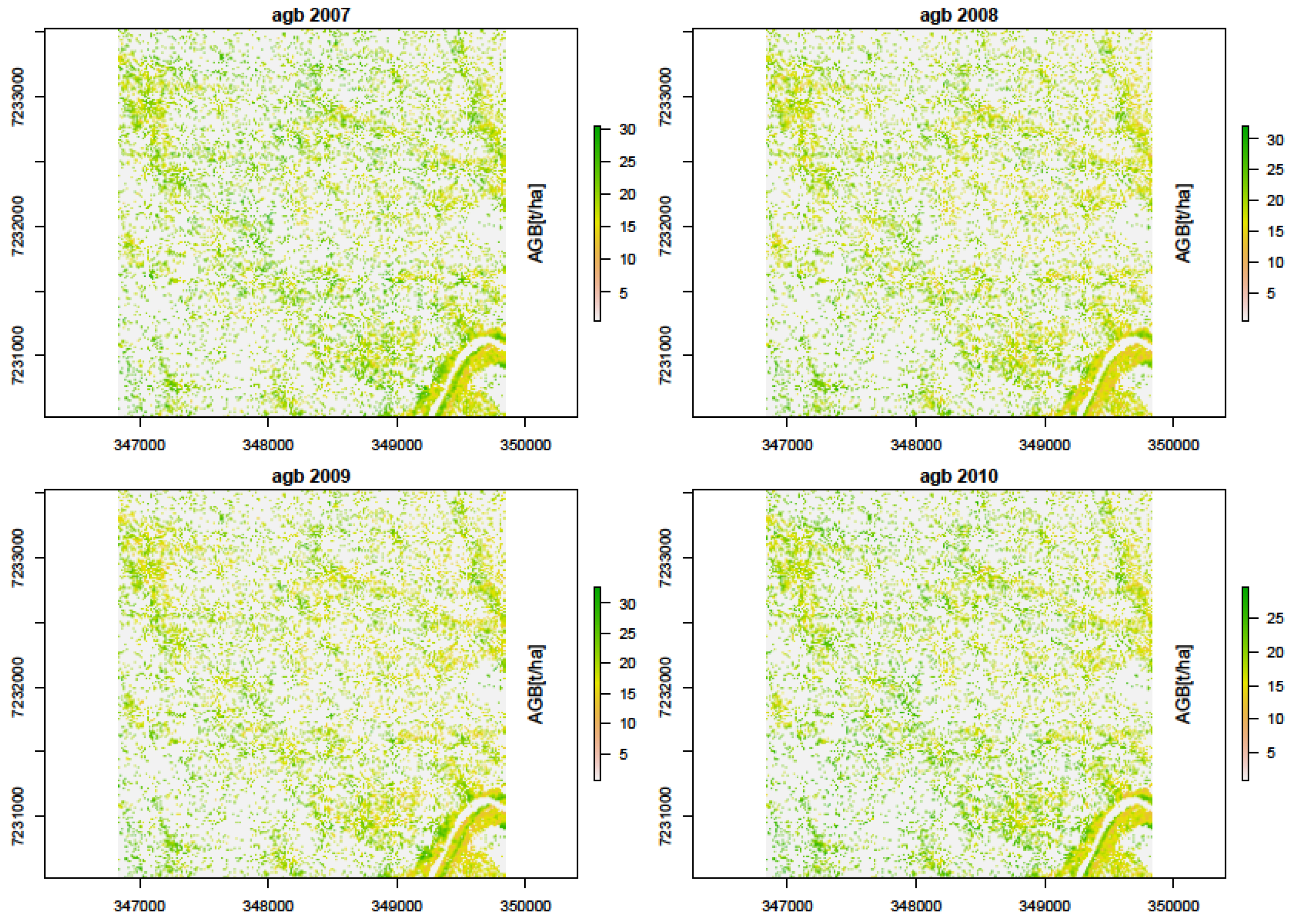
The σ0 values were weighted based on area proportion intersecting the TLS-AGB pixels. A weighted biomass per intersection was then computed. A regression analysis between the σ0 and AGB showed that these two metrics were strongly correlated. We assessed the response of σ0 to AGB in three ways: first we assessed the dual-pol multi-temporal SAR response; second, we assessed polarimetric response (HH and HV)—Figure 12, and lastly, we computed yearly AGB (Figure 13), to assess the multi-temporal (2007 to 2010) SAR backscatter response to AGB. Generally, L-band SAR underestimated AGB, with a mean AGB ± σ of 32.2 ± 14.54 and 32.2 ± 14.29 for SAR co-polarized HH and cross-polarized HV, respectively, in comparison to TLS-metrics derived AGB. Lower AGB estimates were recorded when we combined the polarizations for individual years, with 2007 and 2010 recording the lowest AGB of 19.9 ± 2.6 t/ha and 19.7 ± 5.2 t/ha, respectively. Figure 13 show the biomass maps derived from combined datasets, different polarimetry, and individual years, using RF and linear regression models.
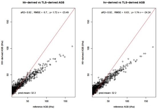
Figure 12.
Correlation between SAR-derived biomass and reference TLS-metrics derived biomass. The graphs show co- and cross polarized L-band ALOS derived AGB responses.
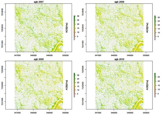
Figure 13.
Predicted woody biomass from SAR backscatter intensity (HH + HV) for the years 2007, 2008, 2009, and 2010.
3.4. Biomass Change Detection
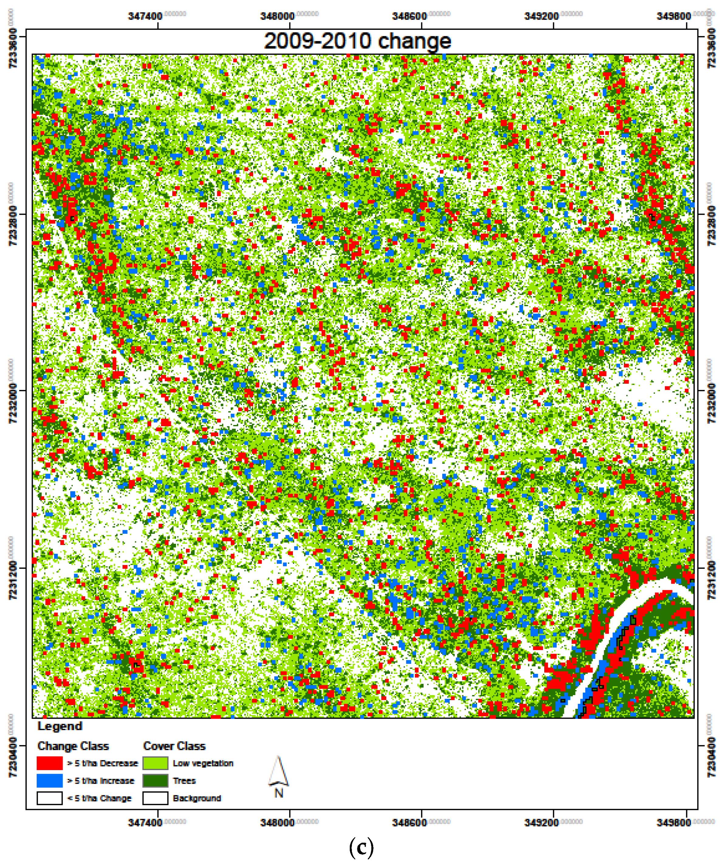
Since all the four SAR-derived AGB datasets were acquired during the dry season and from the same sensor, a comparison of AGB between these years was carried out, with six band differencing combinations. The temporal SAR AGB estimation for the three years yielded AGB ranging between the lowest in 2007 at 19.9 ± 2.6 t/ha and the highest in 2009 at 20.2 ± 4.8 t/ha. We assessed the relative change in AGB within the study area over the four years of study. Generally, there was an observed slight increase in mean AGB between the years 2007 and 2009, but the overlap in the confidence intervals of the estimated AGB over this period makes the increase nonsignificant. We therefore did a relative change analysis over the four years covered by the SAR data to see what the changes were in AGB. First, we classified biomass with 5 t/ha AGB classes, and then assessed the areas within the study area which experienced changes in the AGB with an increase or decrease above 5 t/ha AGB between the years. The results in Table 5 show an overall decrease in AGB, with 3.5% of the study area experiencing a decrease of more than 5 t/ha over the four-year period. Only 3% of the 900 ha study area showed an increase with more than 5 t/ha AGB. Generally, biomass decreased consistently between 2007 and 2009, from 3.3% of the area with an increase >5 t/ha in 2008–2007, to 3.2% in 2009–2008, and finally, a lower 2.6% between 2010 and 2009. Conversely, the study area experienced high biomass reduction with areas experiencing >5 t/ha reduction steadily increasing from 3.2% to 3.3% and finally 4.1% for 2008–2007, 2009–2008, and 2010–2009 combinations, respectively. Over the four year period, more than 90% of the area experienced a change in biomass of less than 5 t/ha. This constitutes areas which experienced a nonsignificant increase or decrease below the 5 t/ha threshold.

Table 5.
Relative change in AGB in Skukuza between 2007 and 2010.
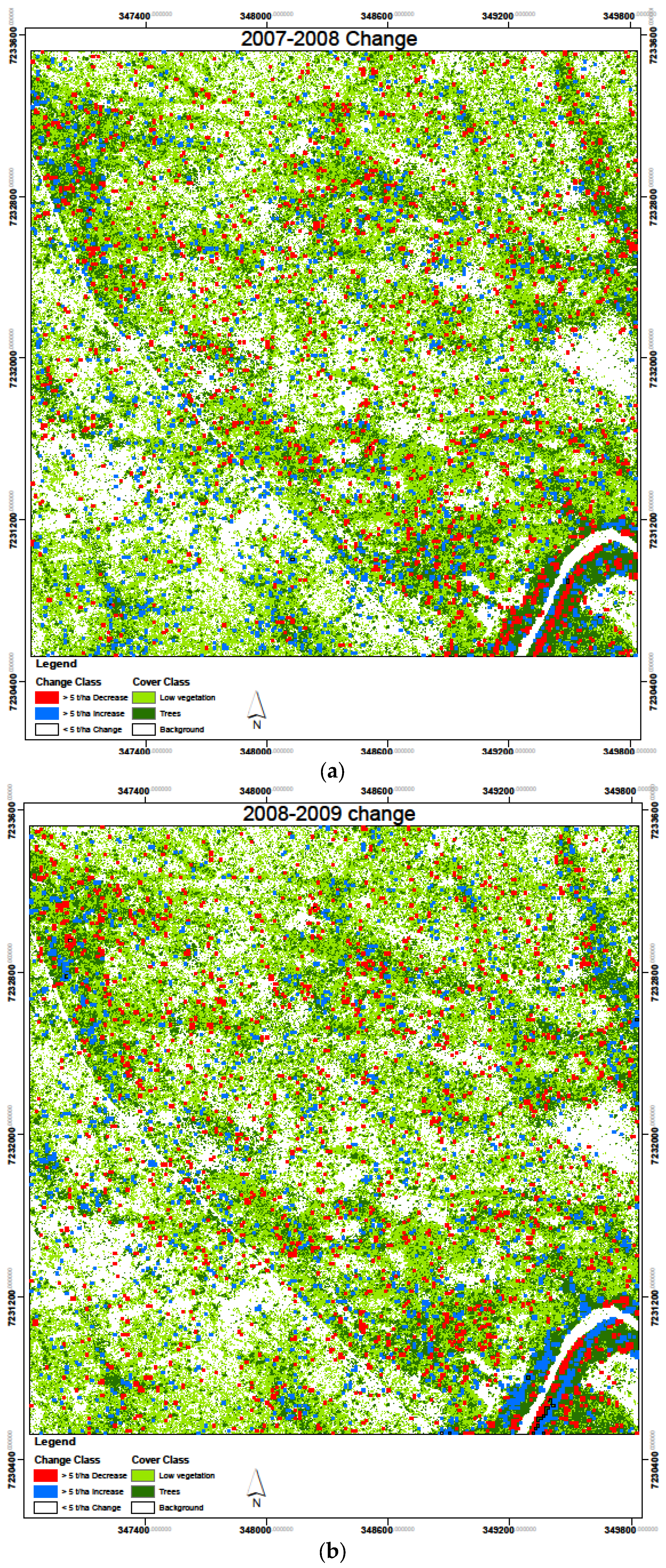
The cumulative change in area with >5 t/ha over the four years, when summed yields a cumulative decrease in AGB within 81.9 ha (9.1%) of the study area where a cumulative increase in AGB occurred within 96 ha (10.6%) of the study area. This shows that, overall, the area with AGB above 5 t/ha was reduced for 32 ha (3.5% of the study area). From the biomass change maps in Figure 14, it is evident that most changes were restricted to the riverine vegetation and along streamlines, areas which are generally covered by woody vegetation. This can be explained by the fact that these areas are the places most likely to have biomass values more than 5 t/ha, and therefore these are the regions where these changes could be detected.
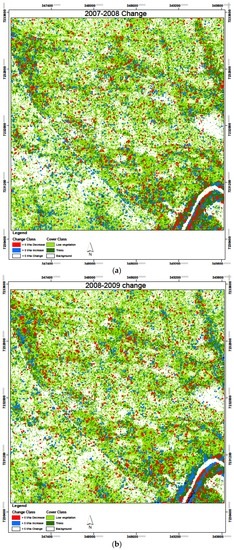
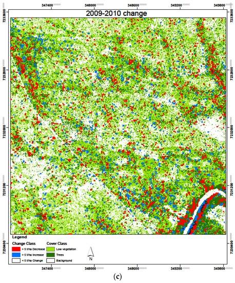
Figure 14.
Biomass change results over the study period 2007–2010, with six change combinations with (a) 2007–2008; (b) 2008–2009; and (c) 2009–2010.
3.5. Uncertainty and Error Analysis
In this study, there are three definite sources of uncertainty: uncertainty in plot mensuration during fieldwork, especially height measurement; uncertainties in using the field data for TLS-derived AGB for the allometric model, and uncertainties in using TLS-derived AGB as reference data for AGB estimation and change detection from SAR backscatter intensity data over a small area. Studies by [76] have pointed to errors associated with field height measurement, as can be seen in Figure 6. Here, an underestimation of tree heights is evident, with lower field inventoried heights correlating better to the TLS height than higher measured heights. This is partly because the accuracy in height measurement using a Laser rangefinder depends on the distance, and the further one moves from the tree to be inventoried, the more difficult it becomes to pinpoint the highest point of a canopy from which the measurement should be taken. A solution would have been to make several measures of the same trees and average such height values. Diameter measurements are usually accurately measured and hence their accuracies are not compromised during field inventories [38]. Biomass model uncertainty in the study emanates from the difference in timing between acquisitions of field and TLS datasets. The former was acquired in the wet season while the latter was acquired in the dry season of the same year. There is error propagation from field-TLS biomass prediction, and using the same as a reference in predicting biomass from SAR. This is visible in the results from Table 4 where the predictions with TLS AGB as reference yields higher RMSE values than the RMSE obtained in its prediction from field-derived biomass. Additionally, SAR datasets lacked appropriate references for accuracy assessment, which further motivated our use of TLS-derived AGB as the reference dataset when modelling AGB from SAR backscatter intensities.
For error analysis, we looked at the residuals (Residual = (У − Ў)) from the fitted regression models—the difference between the reference and predicted or derived aboveground biomass. To assess the assumption of heteroscedasticity in the model residuals which should result in the model residuals being randomly distributed around zero for a range of predicted AGB, we plotted the residuals against the predicted AGB values for TLS and SAR backscatter predictors. This also allowed us to check for systematic bias from the regression models used in predicting AGB.
From the residual plots, the randomness in the points at lower biomass values is evidence of linearity in relationship between the TLS metrics and the field-derived biomass—shown by the scattering of residuals around the zero line. However, this linearity is visible with low biomass values up to 40 t/ha, after which the residual errors increase and become positive in the case of canopy height (CH), and negative in the case of both canopy cover and the product of canopy cover and height (CC and CC × CH). Log-transformation on the field AGB improved the randomness in the distribution of the residuals, and therefore an improvement in the linearity between log-transformed AGB and the predictors can be seen.
4. Discussion
4.1. Distribution of Woody Biomass
The mean woody biomass around the study area from 42 inventoried field plots was 31.86 t/ha (3.1–94.3 t/ha), which is within the range reported by earlier studies in the area [6,15,53], and typical of the Lowveld savanna. From the field mensuration, tree basal diameter was found to be the greatest determinant of woody biomass at plot level, and suffers from fewer introduced errors as opposed to height measurement. However, the basal diameter does linearly correlate to the log-transformed AGB as displayed by the residual plots. L-band SAR data allowed for woody biomass extrapolation over the 9 km2 study area for assessment of area-wide biomass distribution. Despite the underestimation of woody biomass within the study area, SAR backscatter predicted spatial variations in AGB within the study area with a range from 2.9 t/ha in low vegetation areas (typically grass/shrub areas), to 101.6 t/ha around rivers, streams, and areas with clumped trees. These values are within typical biomass ranges reported previously by [6] of 11.9–92.3 t/ha. The spatial distribution of woody biomass around Skukuza is highly variable and this study showed higher biomass values occurring more frequently around seasonal rivers and stream valleys. Studies by [14,75,77,78] have cited soil catenal formations and associated soil and hydrological characteristics as major influences on landscape-scale vegetation structure and compositional variability. This is also visible in biomass change and landcover overlay maps. These areas also display extended vegetation greenness periods slightly beyond the start of the dry season due to water availability [51] and are the areas displaying significant biomass changes above 5 t/ha.
To derive TLS canopy cover and height metrics, we adopted a plot averaging as shown in [79], thereby degrading the spatial resolution of the TLS data from full resolution of 6 cm to the 30 m field inventory plot size. This method, though convenient for estimating each plot’s average biomass, leads to errors as observed by [15], because intrinsic variability among individual trees within the plot are left out. Within this typical Lowveld savanna exists both multi-stemmed and single-stemmed trees, contributing biomass differently based on these metrics, which are in turn affected by non-linearly related biophysical variables.
The L-band SAR data were able to detect both increases and decreases in AGB of >5 t/ha, and the spatial extent of these changes in terms of the proportion of the study area which experienced the reported decrease or increase in biomass of this magnitude. Studies on structural changes in the Lowveld have indicated similar decreases, with [79,80] associating the decreases to fuelwood and timber extractions in settlement areas adjacent to the park. Whereas precipitation is seen as a major limiting factor to savanna structural dynamics, biomass inclusive, it is fire and herbivory that affects vegetation at similar magnitudes at local scales [14,79]. The former affects mainly low shrubs and grass, while the latter, especially browsers, affects mainly woody vegetation. Given the localized scale of this study, and the fact that mostly wooded areas have been affected by the changes, it suffices to conclude that herbivory, especially by elephants (mega-herbivores), is responsible for changes in woody biomass because they push down big trees, thereby modifying both canopy cover and height.
The SAR backscatter intensity values between years vary within similar pixels (and areas) in the study area despite having used data during the dry season within a one-month range (September–October). This would also be helpful in explaining the changes in biomass, and can be attributed to different change agents working in the study area concurrently at different spatial magnitudes. Such would include eco-climatic, topo-edaphic, fire, and herbivory impacts within the study area. These should therefore be investigated over the study period to assess their magnitude of contribution to the biomass dynamics depicted by the change results. A study by [32] suggested correction of effects of moisture to L-band SAR backscatter recalibration of backscatter to ground data at each time point.
4.2. Temporal Dynamics in Woody Biomass
By using multi-temporal SAR data, we were able to detect biomass changes, both decreases and increases within the study area, by estimating the proportional area which experienced a biomass change of more than 5 t/ha over the four years under investigation (Table 5). Generally, the results from the biomass change analysis showed a reduction in biomass over the four years under investigation. This was evident in the cumulative reduction in area that experienced a biomass increase above 5 t/ha. Additionally, the area which saw a reduction in biomass above 5 t/ha increased over the years from 28.8 ha between 2007 and 2008 to 37.3 ha between 2009 and 2010. The biomass change maps also showed these changes restricted to areas with woody vegetation as opposed to shrub/grass areas, with most of these areas around the rivers and streams. The areas with nonsignificant biomass changes (<5 t/ha) were mainly within shrub and grass and bare land cover classes. Changes in shrub and grass classes are attributed to regeneration after fire regimes and saplings from fallen trees [81]. On the other hand, reduction in woody biomass is mainly attributed to mega-herbivores like elephants which knock down big trees. Studies by [82] investigated the effects of megafauna (African elephant) on woody vegetation between 2008 and 2014 in KNP and reported a mean biennial treefall rate of 12% per hectare. This can not only lead to AGB reduction of proportional magnitude but can also lead to a change in land cover, from trees to either shrubs or grass.
4.3. Uncertainties in Biomass Prediction
The error in biomass prediction varies with the method used, with SAR-derived AGB which was not modelled directly from field inventoried data showing lower magnitudes than those modelled with TLS-derived AGB. The allometric validation error (RMSE) from TLS-CHM predictor variables were 4.77 t/ha, 2.13 t/ha and 2.32 t/ha for canopy cover (CC), canopy height (CH), and the product of the two (CC × CH), respectively, constituting 12.5%, 6.3%, and 6.8% of the respective predicted biomass means. The error values are reasonably small even though using the CC × CH biomass with 7% error would lead to error propagation in subsequent predictions as highlighted in this study. The high error values reported in predicting biomass from SAR backscatter are not higher than those obtained within the same area using Nickless allometry [13,14] because the current study used some trees with basal diameter >33 cm. Still, predicted higher biomass values are associated with trees with larger diameters than the ones used in the study. As [83] notes, most allometric models lack large diameter classes and these errors associated with higher values can be explained from the deficiencies in allometries used. This explains the non-linear relationships shown in the residual errors where the prediction gets worse as the biomass gets larger. It is worth noting that the TLS canopy height model, when calibrated and validated by field data, produces small errors.
5. Conclusions
This study examined the potential of upscaling field inventory and TLS data to estimate landscape-wide AGB using L-band SAR data. The complementarities of each of these datasets have been discussed. The field inventory datasets were used to estimate aboveground woody biomass at the plot level, while TLS data helps in increasing the amount of reference data for extrapolation with SAR backscatter over a wider area through regression models. The potential of TLS to estimate AGB as well as the extraction of savanna vegetation structural components like canopy cover and height and their product has been assessed. This study has shown that it is possible to use L-band SAR data to detect biomass changes above 5 t/ha. Whereas these detections were possible with SAR data under outlined accuracy conditions and within the same season in different years, the study did not, however, look at the precise quantities of aboveground biomass loses and gains over the study duration, rather the proportion of the area that experienced a change above the threshold values of 5 t/ha. Future studies should therefore look at quantitative estimation of these changes—this should be possible under similar radar geometries and seasons over multiple years.
The availability of a small TLS footprint, coupled with few field inventoried plots over the study area should be seen as a limiting factor in biomass estimation over the wider study area. This, coupled with multi-resolution datasets used in the study leads to a compromise in utilizing the full potential of TLS data at high resolution. There is a possibility of exploring field biomass inventory at a tree level instead of a plot level. This, when combined with TLS data at full resolution, should go a long way in estimating canopy-level cover and height structure parameters at the tree level as opposed to the plot level.
Acknowledgments
This study was made possible by funding from German Academic Exchange Service (DAAD Ref No. SPACES ST43) under German Federal Ministry of Education and Research (BMBF) funded Adaptive Resilience of Southern Africa Ecosystems (ARS AfricaE) Project (Grant No. 01LL1303D). Funding for the TLS equipment was provided by the Thuringian Ministry of Education, Science and Culture (TMBWK) to Christiane Schmullius (Grant No. 13007-715) with support from the European Regional Development Fund (ERDF). TLS data collection was made possible by funding from German Research Foundation, DFG to Jussi Baade (Grant No. BA 1377-12). Shaun Levick and two anonymous reviewers provided helpful comments to earlier drafts of the manuscript.
Author Contributions
Field data inventory, analysis and manuscript preparation was carried out by the first author. Alecia Nickless helped with insightful information over the study topic, and the interpretation of statistical results. Jussi Baade acquired and processed the TLS raw data over the study area. Mikhail Urbazaev worked on L-band SAR data processing. Christian Walther assisted with processing of the TLS data, while Christian Berger went through the manuscript for corrections. Christiane Schmullius assisted in the field data inventory and supervised the project. All authors contributed helpful comments to the manuscript.
Conflicts of Interest
The authors declare no conflict of interest. The founding sponsors had no role in the design of the study; in the collection, analyses, or interpretation of data; in the writing of the manuscript, and in the decision to publish the results.
References
- Intergovernmental Panel on Climate Change (IPCC). Good Practice Guidance for Land Use, Land-Use Change and Forestry; Glossary 1; IPCC National Greenhouse Gas Inventories Program: Hayama, Japan, 2003. [Google Scholar]
- Gibbs, H.K.; Brown, S.; Niles, J.O.; Foley, J.A. Monitoring and estimating tropical forest carbon stocks: Making REDD a reality. Environ. Res. Lett. 2007, 2, 13. [Google Scholar] [CrossRef]
- Roy, P.S.; Ravan, A.S. Biomass estimation using satellite remote sensing data—An investigation on possible approaches for natural forest. J. Biosci. 1996, 21, 535–561. [Google Scholar] [CrossRef]
- Esser, G. The significance of biospheric carbon pools and fluxes for the atmospheric CO2: A proposal mode structure. Prog. Biometeorol. 1984, 3, 253–294. [Google Scholar]
- Chave, J.; Condit, R.; Aguilar, S.; Hernandez, A.; Lao, S.; Perez, R. Error propagation and scaling for Tropical forest biomass estimates. Philos. Trans. R. Soc. 2004, 359, 409–420. [Google Scholar] [CrossRef] [PubMed]
- Nickless, A.; Scholes, R.J.; Archibald, S. A method for calculating the variance and confidence intervals for tree biomass estimates obtained from allometric equations. Afr. J. Sci. 2011, 107. [Google Scholar] [CrossRef]
- Clark, D.A.; Brown, S.; Kicklighter, D.; Chambers, J.Q.; Thomlinson, J.R.; Ni, J. Measuring net primary production in forests: Concepts and field methods. Ecol. Appl. 2001, 11, 356–370. [Google Scholar] [CrossRef]
- Chave, J.; Andalo, C.; Brown, S.; Cairns, M.A.; Chambers, J.Q.; Eamus, D.; Fölster, H.; Fromard, F.; Higuchi, N.; Kira, T.; et al. Tree allometry and improved estimation of carbon stocks and balance in tropical forests. Oecologia 2005, 145, 87–99. [Google Scholar] [CrossRef] [PubMed]
- Jenkins, J.C.; Chojnacky, D.C.; Heath, L.S.; Birdsey, R.A. National-scale biomass estimatoes for United States tree Species. For. Sci. 2003, 49, 12–35. [Google Scholar]
- Brown, S. Measuring carbon in forests: Current status and future challenges. Environ. Pollut. 2002, 116, 363–372. [Google Scholar] [CrossRef]
- Saatchi, S.S.; Harris, N.L.; Brown, S.; Lefsky, M.; Mitchard, E.T.A.; Salas, W.; Zutta, B.R.; Buermann, W.; Lewis, S.L.; Hagen, S.; et al. Benchmark map of forest carbon stocks in tropical regions accross three continents. Proc. Natl. Acad. Sci. USA 2011, 108, 9899–9904. [Google Scholar] [CrossRef] [PubMed]
- Baccini, A.; Laporte, N.; Goetz, S.J.; Sun, M.; Dong, H. A first map of tropical Africa’s above-ground biomass derived from satellite imagery. Environ. Res. Lett. 2008, 3, 045011. [Google Scholar] [CrossRef]
- Lefsky, M.A.; Harding, D.J.; Keller, M.; Cohen, W.B.; Carabajal, C.C.; Espirito-Santo, F.D.B.; Hunter, M.O.; Oliveria, R., Jr. Estimates of forest canopy height and aboveground biomass using ICESat. Geophys. Res. Lett. 2005, 32, 1–4. [Google Scholar] [CrossRef]
- Colgan, M.S.; Asner, G.P.; Levick, S.R.; Martin, R.E.; Chadwick, O.A. Topo-edaphic controls over woody plant biomass in South African savannas. Biogeosciences 2012, 9, 1809–1821. [Google Scholar] [CrossRef]
- Colgan, S.M.; Asner, G.P.; Swemmer, T. Harvesting tree biomass at the stand-level to assess the accuracy of field and airborne biomass estimation in savannas. Ecol. Appl. 2013, 5, 1170–1184. [Google Scholar] [CrossRef]
- Korpella, I. Individual tree measurements by use of digital aerial photogrammetry. In Silva Fennica Monographs 3; The Finnish Forest Research Institute: Helsinki, Finland, 2004. [Google Scholar]
- Abraham, J.; Adolt, R. Stand Heights Estimations Using Aerial Images and Laser Datasets; Workshop on 3D RS in Forestry: Vienna, Austria, 2006; Volume 2a, pp. 24–31. [Google Scholar]
- Browning, D.M.; Archer, S.R.; Byrne, A.T. Fiel validation of 1930s aerial photography: What are we missing? J. Arid Environ. 2009, 73, 844–853. [Google Scholar] [CrossRef]
- Raumonen, P.; Casella, E.; Calders, K.; Murphy, S.; Akerblom, M.; Kaasalainen, M. Massive-scale tree modelling from TLS data. ISPRS Ann. 2015, 189, 25–27. [Google Scholar] [CrossRef]
- Tilly, N.I. Terrestrial Laser Scanning for Crop Monitoring-Capturing 3D Data of Plant Height for Estimating Biomass at Field Scale. Ph.D. Thesis, University of Köln, Köln, Germany, 2015. [Google Scholar]
- Kandrot, S.M. Coastal Monitoring: A New Approach. Department of Geography, Cork University, Ireland. Available online: http://research.ucc.ie/journals/chimera/2013/00/kandrot/09/en (accessed on 20 June 2016).
- Resop, J.P.; Hession, W.C. Terrestrial laser scanning for monitoring streambank retreat: Comparison with traditional surveying techniques. J. Hydraul. Eng. 2010, 136, 794–798. [Google Scholar] [CrossRef]
- Stanley, T. Assessment of FARO 3D Focus Laser Scanner for forest Inventory. Bachelor’s Thesis, University of Southern Queensland, Toowoomba, Australia, 2013. [Google Scholar]
- Calders, K.; Newnham, G.; Burt, A.; Murphy, S.; Raumonen, P.; Herold, M.; Culvenor, D.; Avitabile, V.; Disney, M.; Armston, J.; et al. Nondestructive estimates of aboveground biomass using terrestrial laser scanning. Methods Ecol. Evol. 2015, 6, 198–208. [Google Scholar] [CrossRef]
- Hackenberg, J.; Wassenberg, M.; Spiecker, H.; Sun, D. Non destructive methods for biomass prediction combining TLS derived tree volume and wood density. Forests 2015, 6, 1274–1300. [Google Scholar] [CrossRef]
- Li, S.; Dragicevic, S.; Castro, F.A.; Sester, M.; Winter, S.; Coltekin, A.; Pettit, C.; Jiang, B.; Haworth, J.; Stein, A.; et al. Geospatial big data handling theory and methods: A review and research challenges. ISPRS J. Photogramm. Remote Sens. 2016, 115, 119–133. [Google Scholar] [CrossRef]
- Liu, J.; Li, J.; Li, W.; Wu, J. Rethinking big data: A review on the data quality and usage issues. ISPRS. J. Photogramm. Remote Sens. 2016, 115, 134–142. [Google Scholar] [CrossRef]
- Warmink, J. Vegetation Density Measurements Using Parallel Photography and Terrestrial Laser Scanning. A Pilot Study in the Duursche en Gamerensche Waard. Master’s Thesis, Department of Geography of Utretch University, Utretch, The Netherlands, 2012. [Google Scholar]
- Rees, W.G. Physical Principles of Remote Sensing, 2nd ed.; Cambridge University Press: Cambridge, UK, 2001; pp. 109–133. [Google Scholar]
- Mitchard, E.T.A.; Saatchi, S.S.; Woodhouse, I.H.; Nangendo, G.; Ribeiro, N.S.; Williams, M.; Ryan, C.M.; Lewis, S.L.; Feldpausch, T.R.; Meir, P. Using satellite radar backscatter to predict above-ground woody biomass: A consistent relationship across four different Africa landscapes. Geophys. Res. Lett. 2009, 36, 1–6. [Google Scholar] [CrossRef]
- Woodhouse, I.H. Introduction to Microwave Remote Sensing; Taylor and Francis: London, UK, 2006; pp. 93–149. [Google Scholar]
- Ryan, C.M.; Hill, T.; Woollen, E.; Ghee, C.; Mitchard, E.; Cassels, G.; Grace, J.; Woodhouse, I.H.; Williams, M. Quantifying small-scale deforestation and forest degradation in African woodlands using radar imagery. Glob. Chang. Biol. 2012, 18, 243–257. [Google Scholar] [CrossRef]
- Le Toan, T.; Beaudoin, A.; Riom, J.; Guyon, D. Relating forest biomass to SAR data. IEEE Trans. Geosci. Remote Sens. 1992, 30, 403–411. [Google Scholar] [CrossRef]
- Antonarakis, A.S.; Saatchi, S.S.; Chazdon, R.L.; Moorcroft, P.R. Using Lidar and radar measurement to constrain predictions of forest ecosystem structure and function. Ecol. Appl. 2011, 21, 1120–1137. [Google Scholar] [CrossRef] [PubMed]
- Treuhaft, R.N.; Chapman, B.D.; dos Santos, J.R.; Goncalves, F.G.; Dutra, L.V.; Graca, P.M.L.A.; Drake, J.B. Vegetation profiles in tropical forests from multibaseline interferometric synthetic aperture radar, field, and lidar measurements. J. Geophys. Res. 2009, 114, 1–16. [Google Scholar] [CrossRef]
- Wijaya, A.; Susanti, A.; Liesenberg, V.; Wardhana, W.; Yanto, E.; Soeprijadi, D.; Mcfarlane, C.; Qomar, N. Leaf area index and biomass assessment over tropical peatland forest ecosystem using ALOS Palsar and ENVISAT ASAR data. In Proceedings of the 5th International Workshop on Science and Applications of SAR Polarimetry and Polarimetric Interferometry (ESRIN), Frascati, Italy, 24–28 January 2011.
- Carreiras, J.M.B.; Vasconcelos, M.J.; Lucas, R.M. Understanding the relationship between aboveground biomass and ALOS PALSAR in the forests of Guinea-Bisau (West Africa). Remote Sens. Environ. 2012, 121, 426–442. [Google Scholar] [CrossRef]
- Adler, D.; Synnott, T.J. Permanent Sample Plot Techniques for Mixed Tropical Forest; Tropical Forest Papers; Oxford Forestry Institute: Oxford, UK, 1992; Volume 25. [Google Scholar]
- Urbazaev, M.; Thiel, C.; Mathieu, R.; Naidoo, L.; Levick, S.R.; Smit, I.P.J.; Asner, P.G.; Schmullius, C. Assessment of the mapping of fractional woody cover in southern African savannas using multi-temporal and polarimetric ALOS PALSAR L-band images. Remote Sens. Environ. 2015, 166, 138–153. [Google Scholar] [CrossRef]
- Kutsch, W.L.; Freibauer, A.; Brümmer, C.; Higgins, S.; Schmullius, C.; Thiel-Clemen, T.; Scholes, R.J.; Archibald, S.; Kirton, A.; Walker, S.; et al. Adaptive Resilience of Southern African Savannas (ARS AfricaE) Proposal Call; German Federal Ministry of Education and Research (BMBF): Bonn, Germany, 2012; pp. 2–3. [Google Scholar]
- Scholes, R.J.; Gureja, N.; Ginannecchinni, M.; Dovie, D.; Wilson, B.; Davidson, N.; Piggott, K.; McLoughlin, C.; van der Velde, K.; Freeman, A.; et al. The environmental and vegetation of the flux measurement site near Skukuza, Kruger National Park. Koedoe 2001, 44, 73–83. [Google Scholar] [CrossRef]
- Kutsch, W.L.; Hanan, N.; Scholes, B.; McHugh, I.; Kubheka, W.; Eckhardt, H.; Williams, C. Response of Carbon fluxes to water relations in a savanna ecosystem in South Africa. Biogeoscience 2008, 5, 1797–1808. [Google Scholar] [CrossRef]
- Scholes, R.J.; Archer, S.R. Tree-grass interactions in savannas. JSTOR Annu. Rev. Ecol. Syst. 1997, 28, 517–544. [Google Scholar] [CrossRef]
- Merbold, L.; Ardö, J.; Arneth, A.; Scholes, R.J.; Nouvellon, Y.; de Grandcourt, A.; Archibald, S.; Bonnefond, J.M.; Boulain, N.; Brueggemann, N.; et al. Precipitation as driver of carbon fluxes in 11 African ecosystems. Biogeosciences 2009, 6, 1027–1041. [Google Scholar] [CrossRef]
- Woodward, F.I.; Lomas, M.R. Simulating vegetation processes along the Kalahari Transect. Glob. Chang. Biol. 2004, 10, 383–392. [Google Scholar] [CrossRef]
- Hüttich, C.; Herold, M.; Wegmann, M.; Cord, A.; Strohbach, B.; Schmullius, C.; Dech, S. Assessing effects of temporal compositing and varying observation periods for large-area land cover mapping in semi-arid ecosystems: Implications for global monitoring. Remote Sens. Environ. 2011, 115, 2445–2459. [Google Scholar] [CrossRef]
- Gesner, U.; Machwitz, M.; Conrad, C.; Dech, S. Estimating the fractional cover of growth forms and bare surface savannas. A multi resolution approach based on regression tree ensambles. Remote Sens. Environ. 2013, 129, 90–102. [Google Scholar] [CrossRef]
- Moses, A.C.; Mathieu, R.; Asner, G.P.; Naidoo, L.; van Aardt, J.; Ramoelo, A.; Debba, P.; Wessels, K.; Main, R.; Smit Izak, P.J.; et al. Mapping tree species composition in Southern African savannas using integrated airborne spectral and LiDAR system. Remote Sens. Environ. 2012, 125, 214–226. [Google Scholar]
- Mistry, J. World Savannas. Ecology and Human Use; Pearson Education: Harlow, UK, 2000; pp. 1–25. [Google Scholar]
- Scanlon, T.M.; Albertson, J.D. Canopy scale measurements of CO2 and water vapour exchange along a precipitation gradient in Southern Africa. Glob. Chang. Biol. 2004, 10, 329–341. [Google Scholar] [CrossRef]
- Scholes, R.J.; Dowty, P.R.; Caylor, K.; Parsons, D.A.B.; Frost, P.G.H.; Shugart, H.H. Trends in savanna structure and composition along an aridity gradient in the Kalahari. J. Veg. Sci. 2002, 13, 419–428. [Google Scholar] [CrossRef]
- Sankaran, M.; Hanan, N.P.; Scholes, R.J.; Ratnam, J.; Augustine, D.J.; Cade, B.S.; Gignoux, J.; Higgins, S.I.; Le Roux, X.; Ludwig, F.; et al. Determinants of woody cover in African savannas. Nature 2005, 438, 846–849. [Google Scholar] [CrossRef] [PubMed]
- Mograbi, P.J.; Erasmus, B.F.; Witkowski, E.T.F.; Asner, G.P.; Wessels, K.J.; Mathieu, R.; Knapp, D.E.; Martin, R.E.; Main, R. Biomass increase go under cover: Woody vegetation dynamics in South African rangelands. PLoS ONE 2015, 10, e0127093. [Google Scholar] [CrossRef] [PubMed]
- RIEGL VZ 1000 Data Sheet. 2015. Available online: http://www.riegl.com/uploads/tx_pxpriegldownloads/DataSheet_VZ-1000_2015-03-24.pdf (accessed on 7 April 2016).
- Baade, J.; Schmullius, C. TanDEM-X IDEM precision and accuracy assessment based on a large assembly of differential GNSS measurements in Kruger National Park, South Africa. ISPRS J. Photogramm. Remote Sens. 2016, 119, 496–508. [Google Scholar] [CrossRef]
- Isenburg, M. LAStools—Efficient Tools for LiDAR Processing, version 111216; Rapidlasso GmbH: Gilching, Germany, 2016; Available online: http://lastools.org (accessed on January–June 2016).
- Khosravipour, A.; Skidmore, A.K.; Isenburg, M.; Wang, T.; Hussin, Y.A. Generating pit-free canopy height models from airborne Lidar. Photogramm. Eng. Remote Sens. 2014, 80, 863–872. [Google Scholar] [CrossRef]
- Lim, K.; Treitz, P.; Baldwin, K.; Green, J. Lidar remote sensing of biophysical properties of tolerant northern hardwood forests. Can. J. Remote Sens. 2003, 29, 658–678. [Google Scholar] [CrossRef]
- Ben-Arie, J.R.; Hay, G.J.; Powers, R.P.; Castilla, G.; St-Onge, B. Developing of a pit filling algorithm for LIDAR canopy height models. Comput. Geosci. 2009, 35, 1940–1949. [Google Scholar] [CrossRef]
- American Society for Photogrammetry & Remote Sensing (ASPRS). LAS Specification, version 1.4-R6; American Society for Photogrammetry & Remote Sensing: Bethesda, MD, USA, 2011; p. 10. [Google Scholar]
- Naidoo, L.; Mathieu, R.; main, R.; Kleynhaus, W.; Wessels, K.; Asner, G.; Leblon, B. Savanna woody structure modeling and mapping using multi-frequency (X-, C- and L-band) synthetic aperture radar data. ISPRS J. Photogramm. Remote Sens. 2015, 105, 234–250. [Google Scholar] [CrossRef]
- GAMMA Remote Sensing AG. Differential interferometry and geocoding software. In Geocoding and Image Registration Documentation User’s Guide; Gamma, R.S., Ed.; GAMMA Remote Sensing: Gümligen, Switzerland, 2008. [Google Scholar]
- Oliver, C.; Quegan, S. Understanding Synthetic Aperture Radar Images; SciTech Publishing: Raleigh, NC, USA, 2004. [Google Scholar]
- Argenti, F.; Lapini, A.; Alparone, L.; Bianchi, T. A tutorial on speckle reduction in Synthetic Aperture Radar images. IEEE Geosci. Remote Sens. Mag. 2013, 1, 6–35. [Google Scholar] [CrossRef]
- Castel, T.; Beaudoin, A.; Stach, N.; Stussi, N.; Le Toan, T.; Durand, P. Sensitivity of space-borne SAR data to forest parameters over sloping terrain theory and experiment. Int. J. Remote Sens. 2001, 22, 2351–2376. [Google Scholar] [CrossRef]
- Stussi, N.; Beaudoin, A.; Castel, T.; Gigord, P. Radiometric correction of multiconfiguration spaceborne SAR data over hilly terrain. In Proceedings of the 1st International Workshop on Retrieval of Bio- and Geophysical Parameters from SAR Data for Land Applications, Centre National D’etudes Spatiales (CNES), Toulouse, France, 10–13 October 1995.
- Trimble eCognition Trainings. Available online: http://community.ecognition.com/home/training-material (accessed on 10 January 2016).
- Chai, T.; Draxler, R.R. Interactive comment on “Root mean square error (RMSE) or mean absolute error (MAE)?”. Geosci. Model Dev. 2014, 7, 589–590. [Google Scholar]
- Breiman, L.; Friedman, J.H.; Olshen, R.A.; Stone, C.I. Classification and Regression Trees; Taylor & Francis: Belmont, CA, USA, 1984. [Google Scholar]
- Breiman, L. Random Forest. Mach. Learn. 2001, 45, 5–32. [Google Scholar] [CrossRef]
- Liaw, A.; Wiener, M. Classification and regression by random forest. R News 2002, 2–3, 18–22. [Google Scholar]
- Odipo, V.O.; Luck, W.; Berger, C.; Schmullius, C. Savanna fractional cover classification using machine learning. Unpublished work. 2016. [Google Scholar]
- Smit, I.P.J.; Smit, C.F.; Govender, N.; van der Linde, M.; Macfayden, S. Rainfall, geology and landscape position generates large-scale spatiotemporal fire pattern heterogeneity in an African savanna. Ecography 2013, 36, 447–459. [Google Scholar] [CrossRef]
- Scholtz, R.; Kiker, G.A.; Smit, I.P.J.; Venter, F.J. Identifying drivers that influence the spatial distribution of woody vegetation in Kruger National Park, South Africa. Ecosphere 2014, 5. [Google Scholar] [CrossRef]
- Baldeck, C.A.; Colgan, M.S.; Feret, J.B.; Levick, S.R.; Martin, R.E.; Asner, G.P. Lanscape-scale variation in plant community composition of an African Savanna from airborne species mapping. Ecol. Appl. 2014, 24, 84–93. [Google Scholar] [CrossRef] [PubMed]
- Mitchard, E.T.A.; Saatchi, S.S.; Lewis, S.L.; Feldpausch, T.R.; Woodhouse, I.H.; Sonke, B.; Rowland, C.; Meir, P. Measuring biomass changes due to woody encroachment and deforestation/degradation in a forest-savanna boundary region of Central Africa using multi-temporal L-band radar backscatter. Remote Sens. Environ. 2011, 115, 2861–2873. [Google Scholar] [CrossRef]
- Levick, S.R.; Asner, G.P.; Chadwick, O.A.; Khomo, L.M.; Rogers, K.H.; Hartshorn, A.S.; Kennedy-Bowdoin, T.; Knapp, D.E. Regional insight into savanna hydrogeomorphology from termite mounds. Nat. Commun. 2010, 1, 1–7. [Google Scholar] [CrossRef] [PubMed]
- Scholes, R.J.; Walker, B.H. An African Savanna: Synthesis of the Nylsvley Study; Ambridge University Press: Cambridge, UK, 1993. [Google Scholar]
- Banks, D.J.; Griffin, N.J.; Shackleton, C.M.; Mavrandonis, J.M. Wood supply and demand around two rural settlements in a semi-arid savanna. Biomass Bioenergy 1996, 11, 319–331. [Google Scholar] [CrossRef]
- Wessels, K.J.; Colgan, M.S.; Erasmus, B.F.N.; Asner, G.P.; Twine, W.C.; Mithieu, R.; van Aardt, J.A.N.; Fisher, J.T.; Smit, I.P.J. Unsustainable fuelwood extraction from South African savannas. Environ. Res. Lett. 2013, 8, 014007. [Google Scholar] [CrossRef]
- Wilgen, B.W.; Trollope, W.S.W.; Biggs, H.C.; Potgieter, A.L.F.; Brockett, B.H. Fire as a driver of ecosystem variability. In The Kruger Experience. Ecology and Management of Savanna Heterogeniety; Du Toit, J.T., Rogers, K.H., Biggs, H.C., Eds.; Island Press: London, UK, 2003; p. 149. [Google Scholar]
- Asner, G.P.; Vaughn, N.; Smit, I.P.J.; Levick, S. Ecosystem-scale effects of megafauna in African savannas. Ecography 2016, 39, 240–252. [Google Scholar] [CrossRef]
- Sankaran, M.; Ratnam, J.; Hanan, N.P. Tree-grass coexistence in savannas revisited-insights from an examination of assumptions and mechanisms invoked in existing models. Ecol. Lett. 2004, 7, 480–490. [Google Scholar] [CrossRef]
© 2016 by the authors; licensee MDPI, Basel, Switzerland. This article is an open access article distributed under the terms and conditions of the Creative Commons Attribution (CC-BY) license (http://creativecommons.org/licenses/by/4.0/).

