1. Introduction
Real-time data analysis using Global Navigation Satellite System (GNSS) positioning coupled with data communication over radio frequencies (RF), or GNSS-RF, is an area of increasing interest in harvest operations as this new technology creates opportunities for innovation in operational forestry. Real-time data analysis and decision support may also be useful in the context of woody biomass logistics as new markets for forest residues and salvage wood develop. Increased interest in emerging and existing bioenergy markets is closely linked with reducing the risks that forested lands face from fire, insects, and pathogens [
1]. It has been estimated that 15 western states in the US contain over 11 million hectares of forested land that could benefit from treatments to improve resilience and health by initiating active forest management on the landscape [
2]. In order to return stands to historic stand dynamics and improve forest health, silvicultural treatments need to be performed, even in stands where such treatments generate large amounts of residues and primarily yield low value products [
3].
Despite increased interest and developing markets, and because biomass products from forest residues are generally low in value, landowners and contractors must develop efficient, effective, and sustainable methods for harvesting and gathering forest residues and beetle-killed timber or the long-term feasibility of supporting new wood-based bioenergy markets will be limited [
4]. By 2022, it is estimated that 12.4 million dry tons of forest residues will be available annually to be utilized for bio-energy [
5]. Higher production rates and lower costs associated with logging systems used in silvicultural systems for salvage and forest restoration operations, including the gathering and processing of other forest residues, will allow forest managers to treat more forest land at lower costs and access a higher proportion of this available biomass feedstock. Not only could this result in healthier forests, but the increased feedstock supply for bioenergy and bio-based product manufacturing could help bolster the economies in communities that rely heavily on the forest products industry. Historically in the US, forest residues have been the primary fuel for bioenergy production, with industrial process heat and power production from forest biomass representing a large portion of overall renewable energy production. Epidemic outbreaks of the mountain pine beetle (
Dendroctonus ponderosae Hopkins) and subsequent mortality of millions of hectares of lodgepole pine (
Pinus contorta var.
latifolia Engelm.) in the northern Rocky Mountains has led to an increased interest in utilizing associated biomass as a bioenergy feedstock option [
6]. Identifying harvesting and processing methods that increase production efficiency and reduce costs through real-time positional analysis of operational equipment and workers may increase the feasibility of using forest residues from treatments in beetle-killed timber, as well as improve overall operational efficiency. Harvesting these degraded beetle-killed stands helps promote the reintroduction of healthy, sustainable forests. The ability to accurately define specific machine elements from spatial data acquired from GNSS-RF transponders is a necessary and first step for the development of real-time production analysis and operator decision-support models that would help achieve these goals.
In the western US, a major potential supply of biomass is thinning residues and other materials removed from fuel treatment operations that occur on US national forests [
7]. Incorporating GNSS-RF technologies in innovative ways in the forest industry may assist operations foresters and contractors in determining the best processes and methods for timber harvesting through real-time positioning and production logistic modeling, especially in beetle-kill. For example, real-time analysis can help to optimize on-the-fly skid trail layout, the order of harvesting, skidding, and processing, and placement of intermediate feedstock preprocessing depot locations.
The on-board data loggers that are standard equipment in many modern forest machines record several types of data that may be useful for real-time analysis of production, such as log piece size and numbers of stems processed [
8,
9]. The addition of discrete equipment position, navigation, and timing (PNT) information to the standard data stream would make it possible for operators to account for and adapt to unforeseen delays in machine cycles or site conditions. Experienced operators do this naturally over short time steps on the fly, but computer-aided analysis can help expose patterns in operation that are not always apparent, even to the most experienced personnel. Utilization of real-time position data for individual pieces of equipment and among multiple pieces of equipment in a system could make it possible for higher resolution and higher order complexity operational models that monitor individual equipment cycle elements and suggest efficiency improvements based on variables like terrain, timber quality, and other site characteristics [
8,
9].
GNSS technology has been studied and in some cases employed in operational forestry contexts including thinning stands, tracking movements of site preparation machinery, aligning logging roads, and positioning and dispatching log trucks along haulage routes in real-time, as well as characterizing soil disturbances related to harvest operations [
10,
11,
12,
13]. Recently, the use of real-time positioning systems in forestry that employ integrated Global Navigation Satellite System (GNSS) and radio frequency (RF) devices is growing, and is important for the advancement and development of operational precision forestry [
14,
15]. Precision forestry is an intensive management technique that emphasizes development of operational practices that incorporate technologies and processes to increase productivity, reduce costs, and reduce negative site impacts, especially those on vegetation, soil, and water resources. Advancements in GIS, GNSS, light detection and ranging (LiDAR), real-time analysis, and most recently GNSS-RF has led to increased interest and application of precision forestry techniques. The innovative application of these new technologies opens the door for advancements in operational forestry by increasing efficiencies of forest management activities [
11,
13]. GNSS uses satellites from the U.S. Global Positioning System (GPS), the Russian global navigation satellite system (GLONASS), and possibly other satellite systems to offer spatial reference data to GNSS receivers around the world. Positioning relies on GNSS receiver ability to communicate with satellite systems to provide location data and is used widely across the globe in consumer, military, and industrial applications. RF are electromagnetic wave frequencies in the range commonly used for communication and radar signals. When GNSS is paired with RF (GNSS-RF) the resultant system has the capability to utilize multiple GNSS-RF transponders that receive positional data through GNSS signals and then instantaneously relay information through RF devices to a receiver. Additionally, communication between transponders and receivers is not reliant on cellular networks nor internet connectivity [
14]. This is especially important for real-time positioning applications in forest operations, which often occur in remote areas with limited cellular network coverage.
Earlier work has primarily focused on GNSS positioning technologies that relay the location of equipment to a distant computer, as with dispatch systems deployed in transportation [
10] and service monitoring applications included on modern machinery. Real-time systems that communicate equipment and ground-worker locations among one another locally at remote logging sites are an important advancement because the technology opens the door to integrated, simultaneous analysis of data from multiple machines and ground workers interacting with one another within the framework of computer-augmented decision processes, with the objective of improving production logistics and safety [
14,
15].
Past research has returned promising results related to the ability of GNSS receivers to monitor forestry equipment movements, though dense forest canopies are known to increase GNSS error and reduce the ability to collect precise and accurate measurements in dense stands [
10,
16,
17,
18,
19,
20]. Even when accuracy is reduced due to canopy closure, GNSS can be successful when high accuracy in monitoring object movements is not required [
10]. For example, position accuracy to 10 m may be insufficient for safety applications, but acceptable for transportation routing. Landscape topography has also been an obstacle in the use of GNSS in forestry applications due to line of sight obstructions [
21]. McDonald and Fulton used GNSS for elemental analysis of skidder cycles and found that GNSS locations could successfully be used to predict cycle durations and distinguish between different elements within those cycles (e.g., grapple, positioning, and travel), though the system was subject to large errors when compared to clock studies (i.e., manual timing by an observer) with regard to specific element durations [
22]. Operational cycles measured with GNSS agreed with direct observation times 90% of the overall time studied [
22]. Similar accuracies were found when using GNSS transponders to analyze the cycle times of forwarders and when using vibration sensors to assist in the determination of cycle times [
23].
While GNSS data have been effective for capturing the location, movements, and overall cycle times of some forest machinery, researchers have encountered problems when attempting to acquire high levels of accuracy in the analysis of specific productive cycle elements [
22,
23,
24,
25]. Additionally, there has been limited prior research evaluating the quality of productive cycle element characterization using positional information derived from GNSS-RF data. Understanding the accuracies and capabilities of commercially available, consumer-grade GNSS-RF transponders will facilitate development of their application in beetle-killed harvest logistics and in production analysis in forest operations more broadly.
The objective of this study was to determine the effectiveness of multi-transmitter GNSS-RF units for characterizing the cycle elements of a log loader at three intervals of GNSS-RF signal transmission and two locations along the machine boom, using time and positional data sent by the transponders. GNSS-RF positional data were compared statistically to manually recorded time intervals for the same cycle elements. Our goals in determining the accuracy of the technology were two-fold: (1) to foster innovation in operations research, especially in the safe, efficient characterization of cycle elements and continued development of accurate, real-time model-assisted decision support and analysis; and (2) to facilitate the development and deployment of these technologies in the forest sector to improve productive efficiency and reduce costs. These goals are of particular interest and application in improving harvest logistics of beetle-killed timber harvests for biomass when product values are low, potential profit margins are narrow, and cost-minimization, even by small margins, can have large impacts on the financial viability of supply chains.
2. Materials and Methods
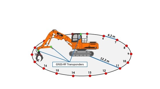
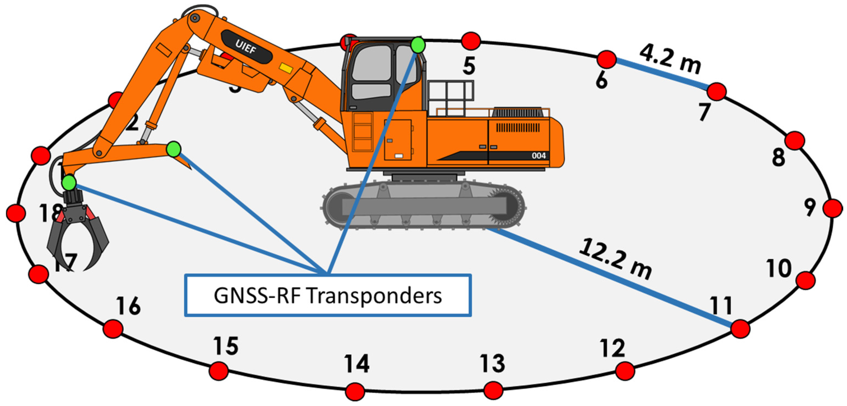
We used Garmin Alpha multi-transmitter GNSS-RF units to record the swing movements of a stationary log loader, also called a “shovel”, in order to characterize the swinging and slew of the boom. This study was conducted on one research site with four replicated trials, with each trial consisting of 18 cycles. The full swing extent of the machine (360 degrees) was broken into 18 equal arc segments of 20 degrees each (
Figure 1). Separation of the swing extent into smaller components made it possible to time the machine movements at varying swing angles to determine if GNSS-RF transponders were able to capture the machine movements accurately at different distances of motion. This was done for three transmission frequency refresh intervals: 2.5, 5.0 and 10.0 s. These three refresh intervals translate into transmission intervals of 24, 12 and 6 transmissions per minute for the 2.5, 5.0 and 10.0 intervals respectively. GNSS-RF transponders were placed in three locations on the machine: one in the right-rear of the cab (close to the center of the machine), one at the full boom extent near the grapple, and one at the heel rack, which is halfway down the most forward boom segment (
Figure 1).
To lay out the experiment, a circle with a radius of 12.2 m was delineated in a flat, open area. The open area was chosen purposefully to avoid attenuated GNSS signals and resulting multipath error. The center point was chosen and a fiberglass tape was extended to the chosen radius or 12.2 m. As the individual at the center point rotated around the axis, a field technician on the end of the tape marked the outside edge with paint. Wooden stakes were placed along the circumference of the circle to mark the 18 different angle segments of 20 degrees each. To determine the location of these points, we determined the side length of an octdecagon (18 sided regular polygon) using the circumradius of 12.2 m and the formula side = 2
r·sin (180/
n), where “
r” is the circumradius, and “
n” is the number of sides. Each side of the polygon measured 4.23 m. A starting point stake labeled “0” was placed on the circumference of the circle. The location of stake 1 was determined by measuring 4.2 m from stake 18 and finding where along this circumference of the circle this landed. This process was repeated for the remaining stakes (2–17) until there were 18 unique 20 degree angle segments within the full swing extent as shown in
Figure 1.
The machine was then driven to the center of the plot and operated in this location for the duration of the study. Keeping the machine in a stationary position removed any possible error or variation that lateral movements would introduce to the GNSS data. The signal sent to the hand held receiver relies on satellite communication to transmit GNSS locations. The number of satellites with which the receiver can communicate at any point in time alters the accuracy of the measurement at that time, meaning accuracy is variable in time depending on how many satellites are in range. We were not able to record the number of satellites in range for each measurement to quantify this source of error. Therefore, a completely randomized design was used in the data collection process, which is described below. A total of seven (7) Alpha multi-transmitter GNSS units were used for the experiment and two (2) handheld receivers were used in data collection. Three Alpha transponders were utilized in measuring the boom movements at the grapple head and were labeled Boom 1, Boom 2 and Boom 3. Boom 1, 2 and 3 were assigned transmission intervals 2.5, 5.0 and 10.0 s, respectively. Three additional Alpha transponders were used in the data collection for the heel rack and labeled Heel 1, Heel 2 and Heel 3 with transmission intervals 2.5, 5.0 and 10.0 s, respectively. One Alpha transponder was labeled as Cab and was used for both the boom and heel trials. The main hypothesis being tested is that shorter transmission intervals result in better accuracy when classifying cycle elements. Additionally, we hypothesized that shorter intervals would also result in more accurate estimates of the angle of machine swing.
The three Alpha transponders attached to grapple and the cab transponder were synched to one handheld receiver. The additional three transponders for the heel and the cab transponder were synched to the second handheld receiver. Two handheld receivers (full and heel) were used as opposed to one receiver to ensure data would not overlap and be compromised. During the swinging experiment, the boom was extended to 9.5 m from the center axis of the log loader and the heel rack was kept a constant 6.7 m from the center axis of the log loader. After each replicated trial, these distances were checked to ensure consistency throughout the experiment. The transponders were easily attached to the heel rack and grapple of the loader with zip-ties, meaning no modifications had to be done to the machinery and the operator could perform tasks normally, with no changes in operation attributable to the addition of the transponders or any other experimental condition.
In each of the four trials, the shovel covered all 18 of the angle segments in separate cycles in random order predetermined by a random number generator. Through each of the 18 cycles per trial, the start time, stop time at the randomly selected angle, and the return time to the start position was recorded both manually and through the data packets received by the GNSS-RF receiver. Manual timing was conducted on a laptop computer using the Sys.time() command in the R statistical programming environment. The internal clock of the laptop used to conduct the manual timing was synched to the time on the GNSS-RF receiver by synchronizing with the
nist.gov time server [
26]. Synching the time of the GNSS-RF receivers and the laptop assisted in matching the GNSS-RF data with the manually recorded cycle times ensuring error when merging manually and remotely collected data was minimized.
Three 4.9 m, beetle-killed lodgepole pine logs were used in the experiment to simulate real world use of the loader on a harvest site. For each of the 18 cycles for each of the four replications, the same sequence was followed. This resulted in 72 unique cycles for both the grapple and heel rack GNSS placements. The logs and log loader boom began at the 0 degree marker to start each cycle. Once the operator swung to the required angle, the logs were dropped and the loaded swing time was recorded. The operator would then swing back to the starting position empty, following the same path. The ending time was recorded when the grapple was placed on the ground back at position 0. At this time the operator would then gather the logs and return them to the 0 degree marker to reset for the next cycle, which always started at position 0. Two cycle elements were defined to represent the movements of the log loader: “Swing/Unload” and “Return”. “Swing/Unload” is described as the time from the start of the swing for each cycle with a loaded grapple starting at angle 0 until the loader drops the logs at the ending angle measure and starts the swing back to the starting point. At this point, the time from the start of the return swing to the moment the grapple touches the ground back at angle 0 is defined as “Return”. The loading element of the cycle, which consists of an unloaded grapple leaving the stop position and collecting logs before the start of the loaded swing element was not included in measurement because it was expected to be identical for each cycle, was not required to test transponder accuracy, and would have introduced additional variation into the timing. Motorola two-way radios were used to communicate with the operator during the experiment, including directions about the selected angle for each cycle.
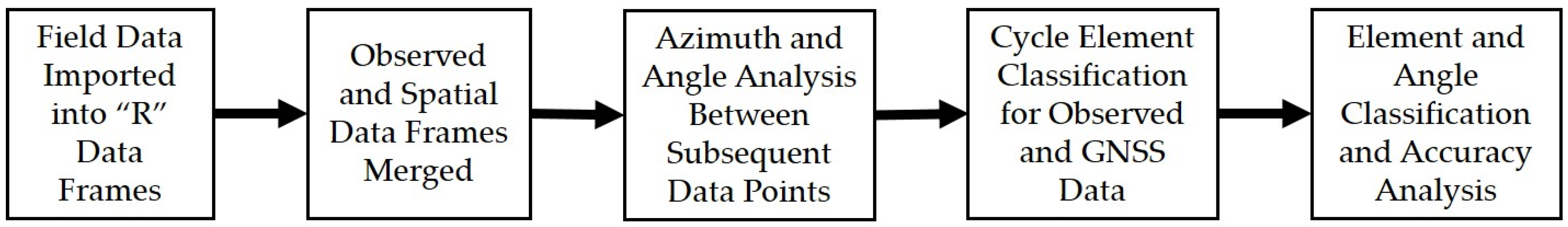
The resulting data from the field observation data sheets and the data received from the Garmin GNSS-RF receivers were entered into a spreadsheet and imported into the statistical analysis environment “R”. The data were then processed, analyzed, and interpreted following the flow diagram represented in
Figure 2.
A chi-squared ANOVA test was performed to determine the significance of each individual parameter on the proportion of correct classifications. The parameters tested included transmission interval, swing angle, transponder location, cycle element, and the interaction of transmission interval and swing angle. Additionally, a binomial logistic regression was used to determine the influence of the predictor variables on cycle element classification of the GNSS data when compared to the field observations. A regression based two-one sided
t-test (TOST) equivalence test was performed to analyze whether the predicted angles of the model derived from GNSS-RF data were statistically similar to the observed angle measures. To further analyze the relationship between observed and predicted angle measures derived from the GNSS-RF data, a linear regression based adapted two-one sided
t-test (TOST) was performed with bootstrapping in order to determine whether the null hypothesis of dissimilarity could be rejected for the observed angle measures and predicted values. Unlike traditional hypothesis testing where a failure to reject null results in a conclusion of indifference, an equivalence test starts with the assumption of dissimilarity, meaning that a rejection of null indicates similarity. This analysis process then shifts the burden of proof onto the model’s ability to derive accurate predictions. Equivalence testing was originally derived from bioequivalence testing used in the development of pharmaceutical drugs, and has been successfully adapted and utilized in tree physiology and biometrics research [
27,
28]. While TOST tests for population-wide agreement, the regression based adaptation discussed by Robinson et al. also addressed point to point agreement between observed and predicted values [
28]. This adapted analysis is able to test how well the distributions of the observed angles match the distribution of the predicted angles. Additionally, the ability to use bootstrap resampling makes this statistical approach favorable. Resampling was not done to provide an estimate of the distribution of the predicted values. The data retrieved from the GNSS-RF data packets and subsequent derivations provided us with the predicted value distribution. Rather, the bootstrap resampling is included to provide an estimate of the sampling distribution within the range of predicted angle measures; providing a larger sample size than could feasibly be obtained in fieldwork alone. The ability to increase sample size can strengthen the evidence for similarity in equivalence-based tests [
28].
All statistical analysis was performed in R [
29]. The equiv.boot function in the “equivalence” package was used to evaluate equivalence tests [
30]. A total of 12 equivalence tests were conducted using 95% confidence intervals. These represented all combinations of the three transmission intervals (3), GNSS-RF transponder locations (2), and cycle elements (2). The equiv.boot function analyzes whether the slope and intercept of the regression of predicted angles fall within the desired region of equivalence, determining similarity or dissimilarity to observed angles. The region of equivalence for the regression was tested at ±10% for both the slope and the intercept and 10,000 bootstrap replications were performed [
28]. Equivalence testing shifts the burden of proof to difference.
4. Discussion
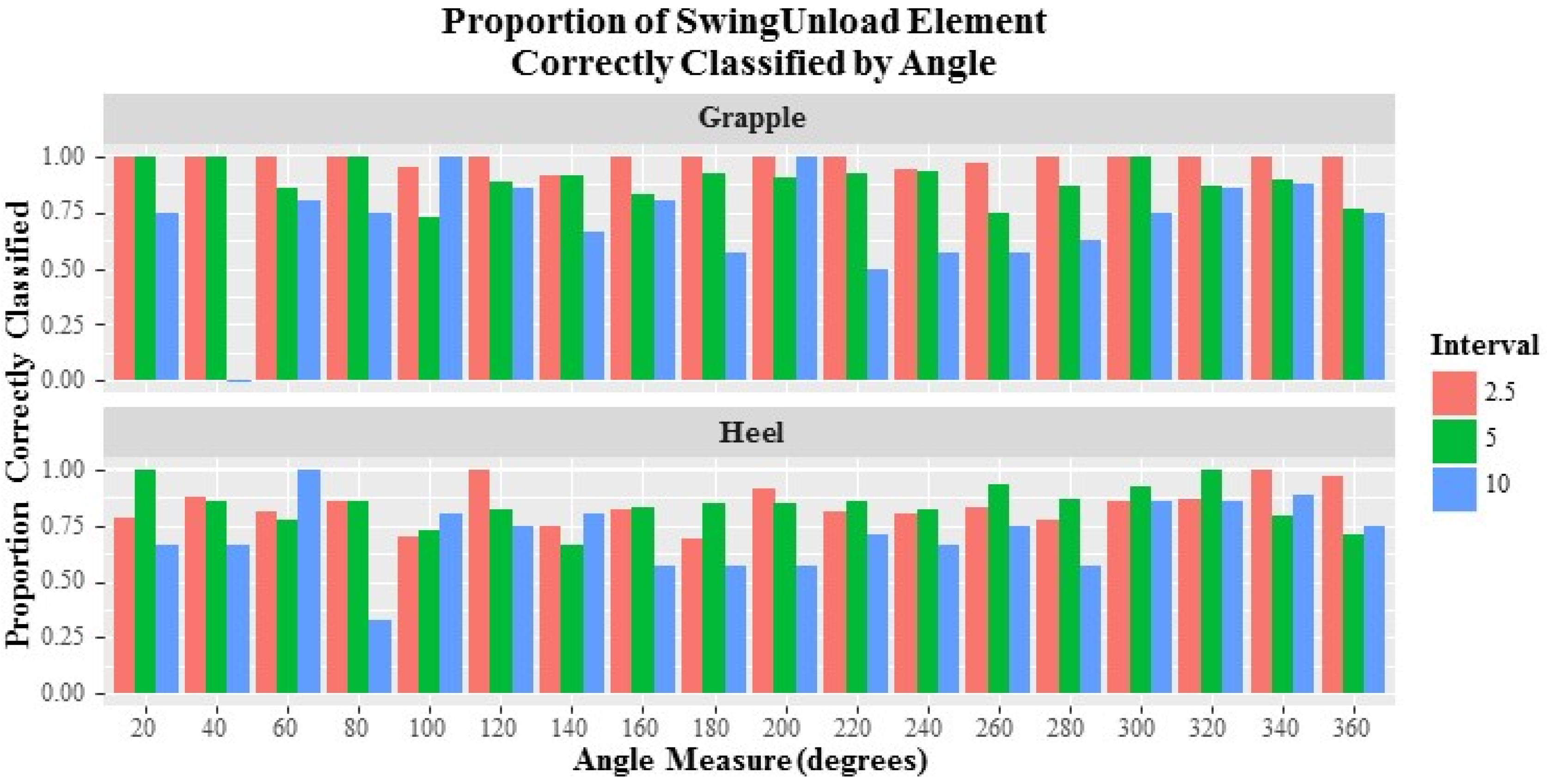
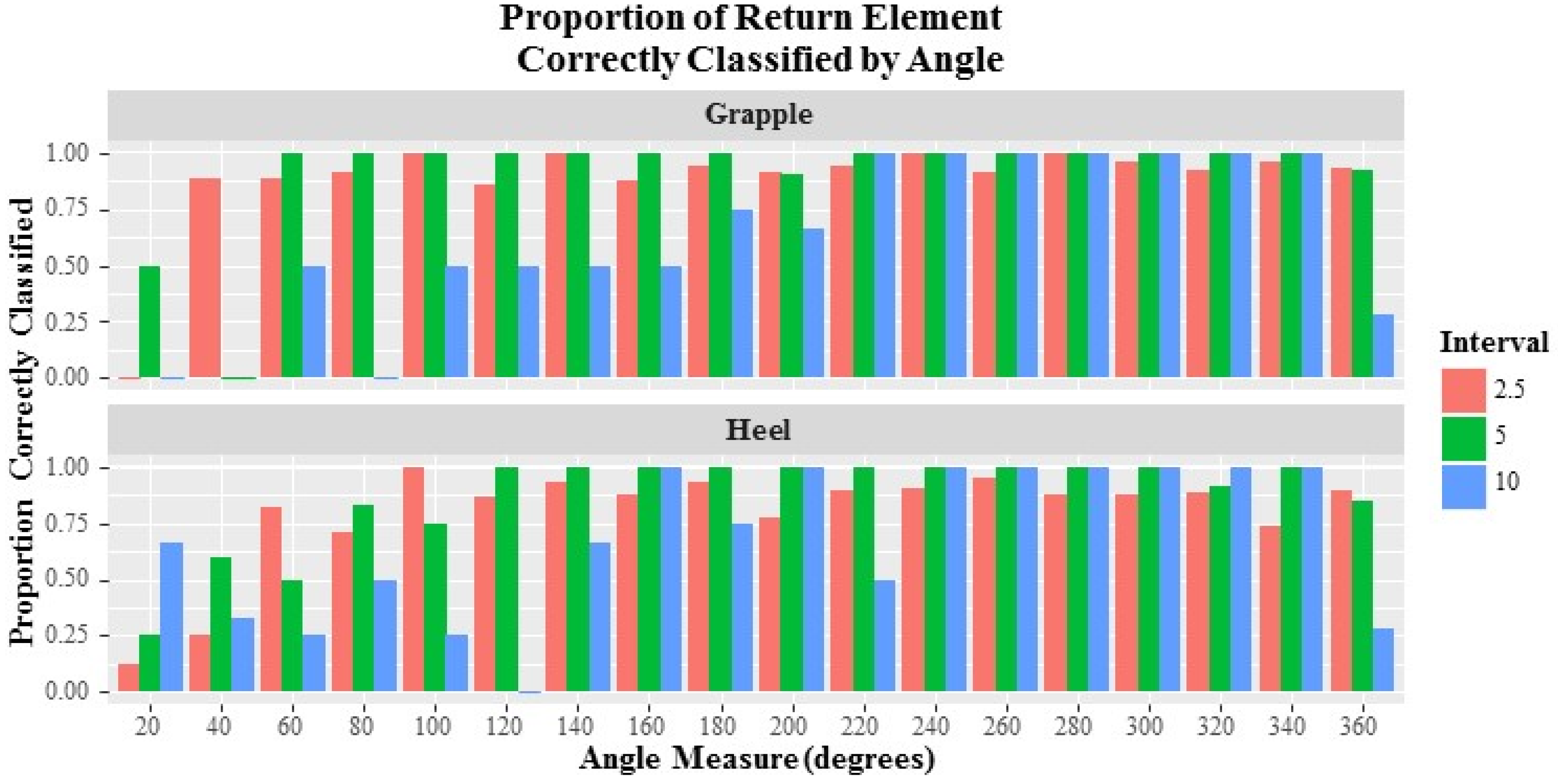
Analysis of the field data returned both expected and surprising results. As anticipated, the 2.5 s transmission interval data returned the highest proportion of correct element classifications. However, the 5.0 s transmission interval returned comparable correctly classified proportions. With 2.5 and 5.0 s transmission intervals capturing 94.4% and 91.7% of the respective overall cycles with at least one correct element for both Swing Unload and Return at the Grapple, accuracy exceeding that described by McDonald and Fulton and similar to that described by Hejazian et al. was obtained when classifying machine cycles using GNSS data [
20,
24]. The ability to correctly classify at least one observation of each element within each trial was reduced when analyzing the Heel data. The associated percentages of success for the 2.5, 5.0 and 10.0 s intervals at the Heel were 91.7%, 88.9% and 58.3%, respectively. Even so, if, for some operational reason, the transponders were placed at the heel rather than the grapple, a transmission interval of 2.5 or even 5.0 s would provide useful data, depending on accuracy requirements.
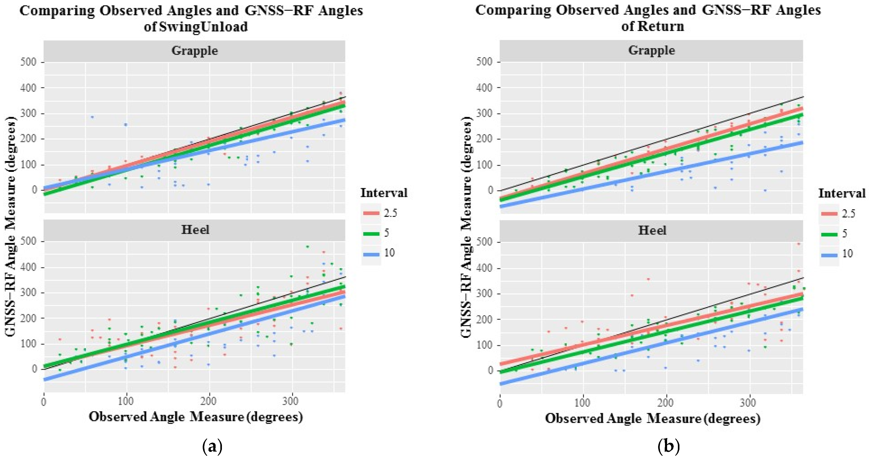
When addressing the potential for GNSS-RF transponders to accurately capture angle measurements, a consistent trend of angle underestimation was found across all angles exceeding 180 degrees, though at the smaller angle measures this underestimation is decreased and in some cases there is predicted angle overestimation (
Figure 5). The reason for this underestimation at the larger observed angle measures is likely due to transponder data packets representing the machine swing not capturing the full extent of the swing arc. For the GNSS location to represent the true arc angle, the transponder has to record a data packet the exact moment the full swing extent is reached or during any pause at the full extent. The time of a pause at full extent is a greater proportion of the overall time at shorter arcs, resulting in a higher inclusion probability of a data packet representing full swing extent. Therefore, the full extent would be represented more often for smaller swing angles and would result in lower underestimation of swing angles. As seen in
Figure 5, any intersection of the 1:1 line and the time interval trend line represents a location where the predicted angles derived from the GNSS-RF data match observed angles. Additionally,
Figure 5 and
Table 4 indicate overall that the 2.5 s interval is most successful in capturing data to derive accurate angle measures.
In our analysis, there was a trend of decreased GNSS measurement accuracy at the Heel location when compared to the Grapple location. The movement of the transponders around a smaller swing circumference means the transponders are less likely to be able to accurately and concisely plot varying points because the range of the movements is shorter. This is due to the inherent accuracy of GNSS. For example, GNSS accuracy of ±1 m will have a greater impact on accurately capturing movements when the overall distance traveled 5 m as opposed to 15 m or 20 m. One possible solution to help account for this error when the swing arc is smaller is to incorporate additional sensors and mechanisms to capture grapple and other intricate movements to assist in defining elements [
8]. These would augment GNSS data in ways that get around constraints related to GNSS accuracy. At the longer GNSS-RF transmission intervals, minute machine boom movements are not as accurately captured. This is seen by observing both the positional data itself, as well as the successful classification proportions. This is especially clear for the 10.0 s interval data. As suggested by Devlin and McDonnell, the 10.0 s interval may be beneficial for analysis of general machine movements across the landscape [
10]. However, precise and intricate machine movements are best captured and analyzed using higher frequency data transmission of locations. Importantly, transmission intervals should be tested and tailored to meet the needs of particular equipment movements rather than relying on a general rule of thumb.
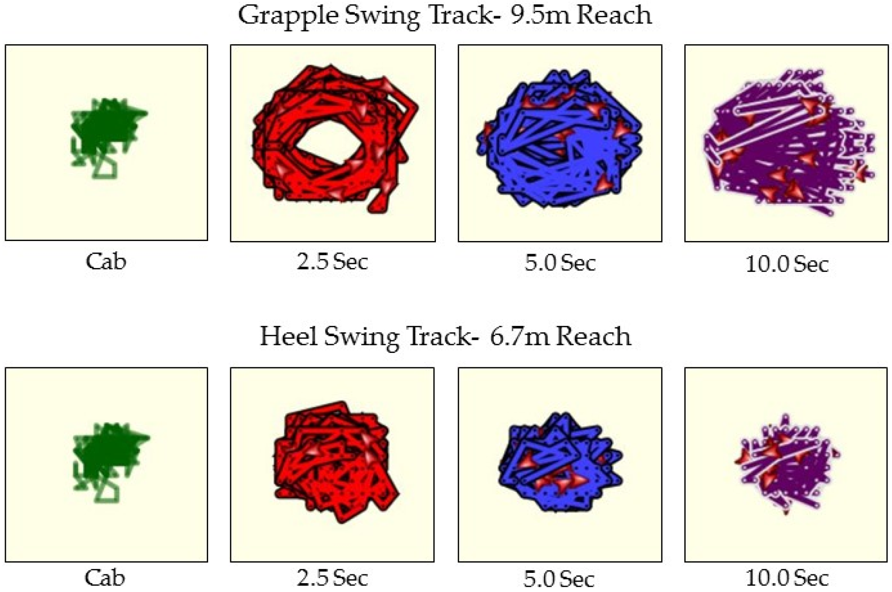
From a visual representation standpoint, it is evident in
Figure 3 that the 2.5 s transmission interval results in a plotted machine movement track that has smoother curves and higher accuracy representation of precise machine movements and machine component locations to meet operational analysis objectives. Correct classification of elements and overall cycles exceeding 90% for the 2.5 s interval further support this observation, as does the results of the regression based equivalence test. However, higher frequency transponder transmission rates are also more data intensive, requiring twice the data flow and storage capacity. This intensity could be difficult to manage for large projects with many pieces of equipment, both in terms of data collection and storage, but also real-time analysis, validation, and model optimization. When addressing the ability of the transponder to accurately characterize machine cycles, cycle elements, and angles of swing, the 5.0 s interval was shown to return comparable accuracies to those obtained by the 2.5 s interval transponders, at half the data intensity.
In this particular study, the overall sampled time represented only a small portion of what a full productive work day would entail in a commercial logging operation in beetle-killed timber. With the 2.5 s interval, the available storage space needed for each data file will be utilized twice as fast as the 5.0 s interval. Each file saved can consist of up to 9999 data points, after which the device overwrites existing data by default. Therefore, a new file needs to be saved on the handheld receiver every 6.9 h when working with the 2.5 s transmission interval to avoid overwriting and every 13.8 h when working with the 5.0 s transmission interval with three transponders. If additional transponders are used on multiple pieces of equipment, then available storage space will be used up more quickly. This can present problems with data being overwritten during average work days if the file is not saved, e.g., mid-way through the day. Additionally, it was found that the large data pools associated with the 2.5 s interval made analysis and interpretation of the data more cumbersome and time intensive than the longer intervals, an observation also made by de Hoop and Duprè [
25]. Depending on the specific application, machines, and desired level of accuracy, incorporating the 5 s interval could return acceptable, though slightly lower, accuracies than the 2.5 s interval. In turn, longer work cycles could be sampled without concern for overwriting data and analysis and interpretation of those data would prove quicker and easier than with the 2.5 s interval if available memory storage and analytical capacity is a concern. When interest is focused on positioning and analysis of precise machine movements where rapid machine movements may be missed by long transmission intervals, the 2.5 s interval likely provides the best option for transmission frequency, or perhaps the study requires more traditional work study methods that relies on direct rather than passive observation.
An important consideration with our study is that the Garmin Alpha receiver and positioning transponders were located in open line-of-sight conditions, which may not be typical of many forest stands. No transmissions were obstructed by vegetation, topography, or inter-machine positioning. One hundred percent of the time-stamped positional coordinates were received. Prior experience with GNSS-RF data in operational forestry has shown that GNSS position and radio signal propagation quality (RSSI) can interact in complex ways. In operational forestry, there are many situations in which positioning transponders may receive a GNSS signal [
14,
15], but radio propagation of coordinates to other devices elsewhere on the jobsite is blocked topographically by dense vegetation or interference from other radio systems [
14,
15]. If a portion of data packets are missing due to radio signal interference, the classification of machine elements may be affected in more complex ways not evident in our controlled experiment. With the quantities of data collected in this way, post-hoc manual and visual inspections of outlier points is almost impossible, so automated data quality control procedures are especially critical in such an environment.
In order to further develop real-time modeling of machine movements on active logging operations, further studies exploring the impacts of forest canopy on GNSS-RF accuracy in particular applications should be explored. For example, in stands with high mortality due to beetle-kill with many trees that have dropped most of their foliage, this may not be a problem, but that remains to be evaluated. Past studies exploring canopy impact in GNSS accuracy have shown large decreases in accuracy depending on canopy cover [
10,
16,
17,
18,
19,
20,
31]. However, these studies were for GNSS only and did not study dual effects of canopy on GNSS and RF, or the interaction of these two signals. Because canopy density tends to be low in beetle impacted stands due to high levels of mortality, for example, canopy impacts on GNSS multipath error may be less of a concern than in healthy stands. Additionally, developing a methodology for similar element and cycle classification when the machine is traversing the landscape on steep slopes in beetle impacted stands in biomass utilization operations as opposed to sitting in a fixed location on flat ground will be necessary. Introducing machine movements on slopes into the analysis will add an additional level of complexity but is important for development of subsequent applications to improve the efficiency of harvesting in beetle impacted and unaffected forests alike.


