Evaluating Inter-Rater Reliability and Statistical Power of Vegetation Measures Assessing Deer Impact

 ,
,
Abstract
:1. Introduction
2. Materials and Methods
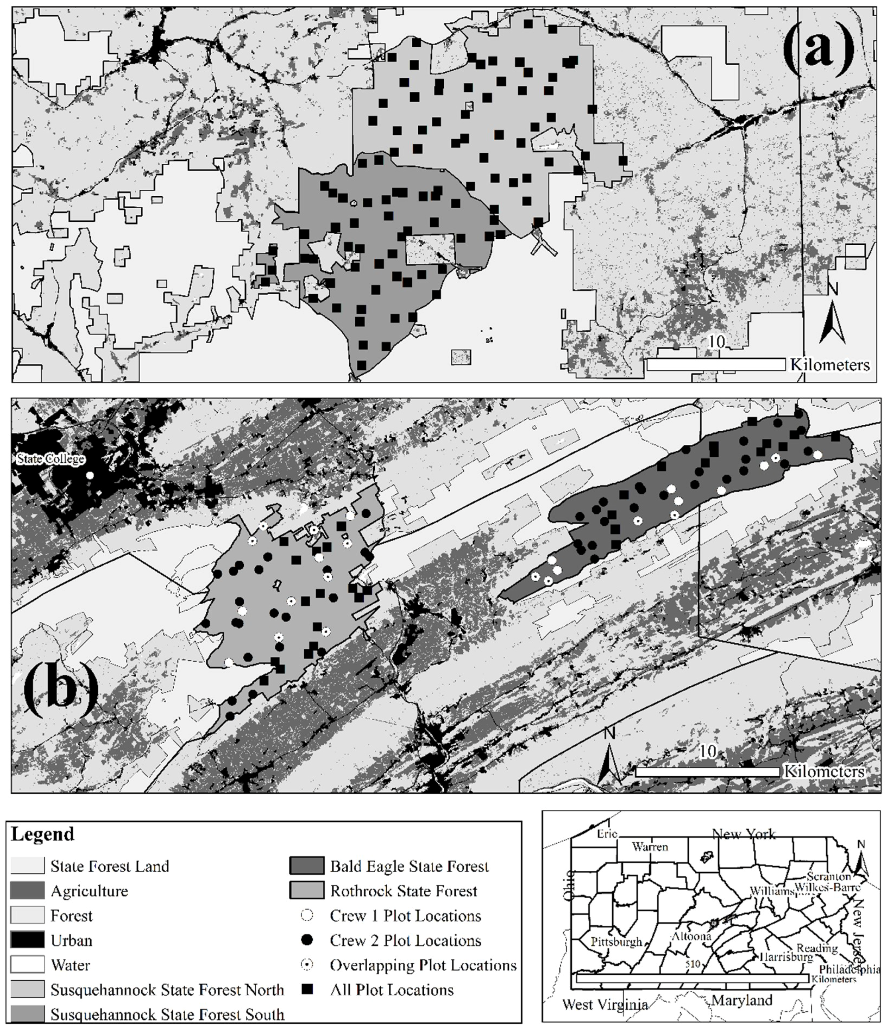
2.1. Study Area Characteristics
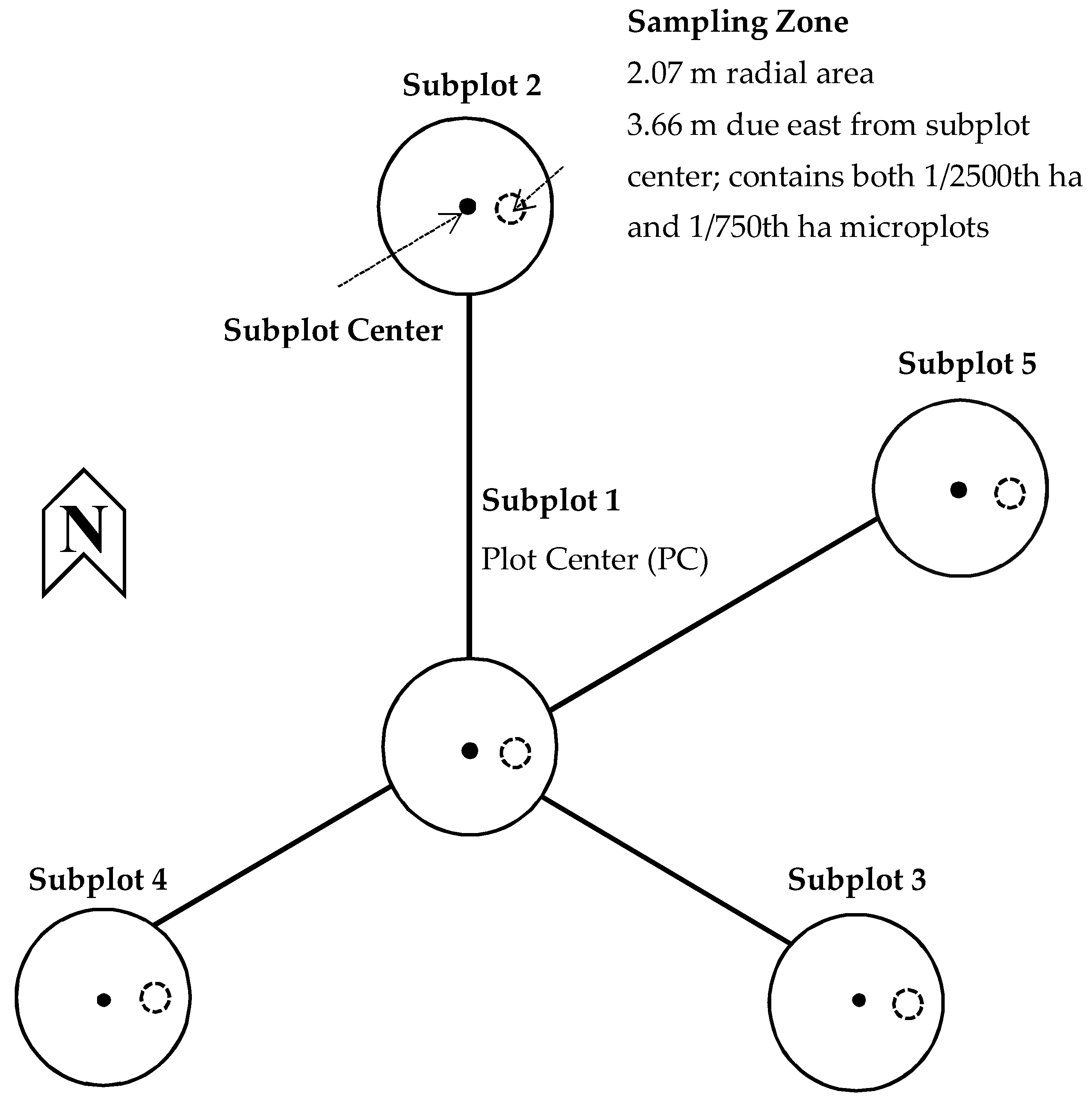
2.2. Vegetation Monitoring
2.3. Data Analysis
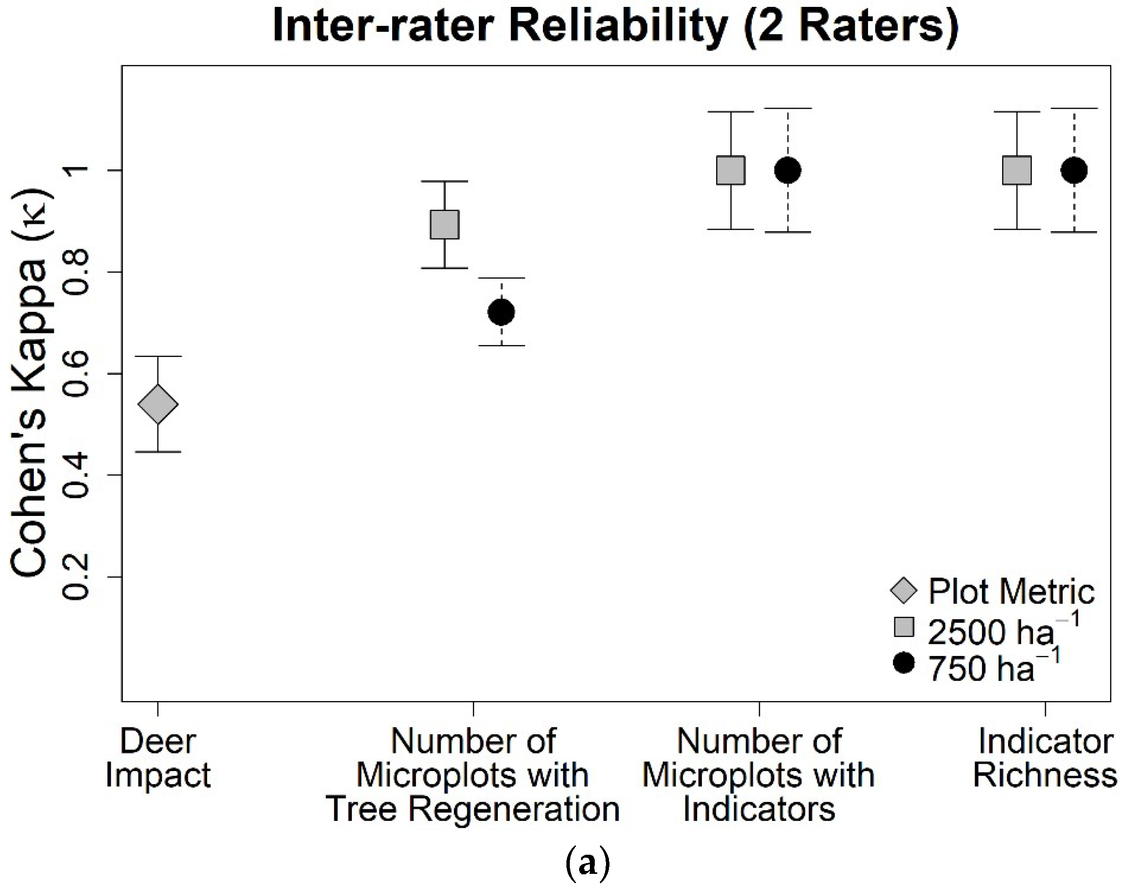
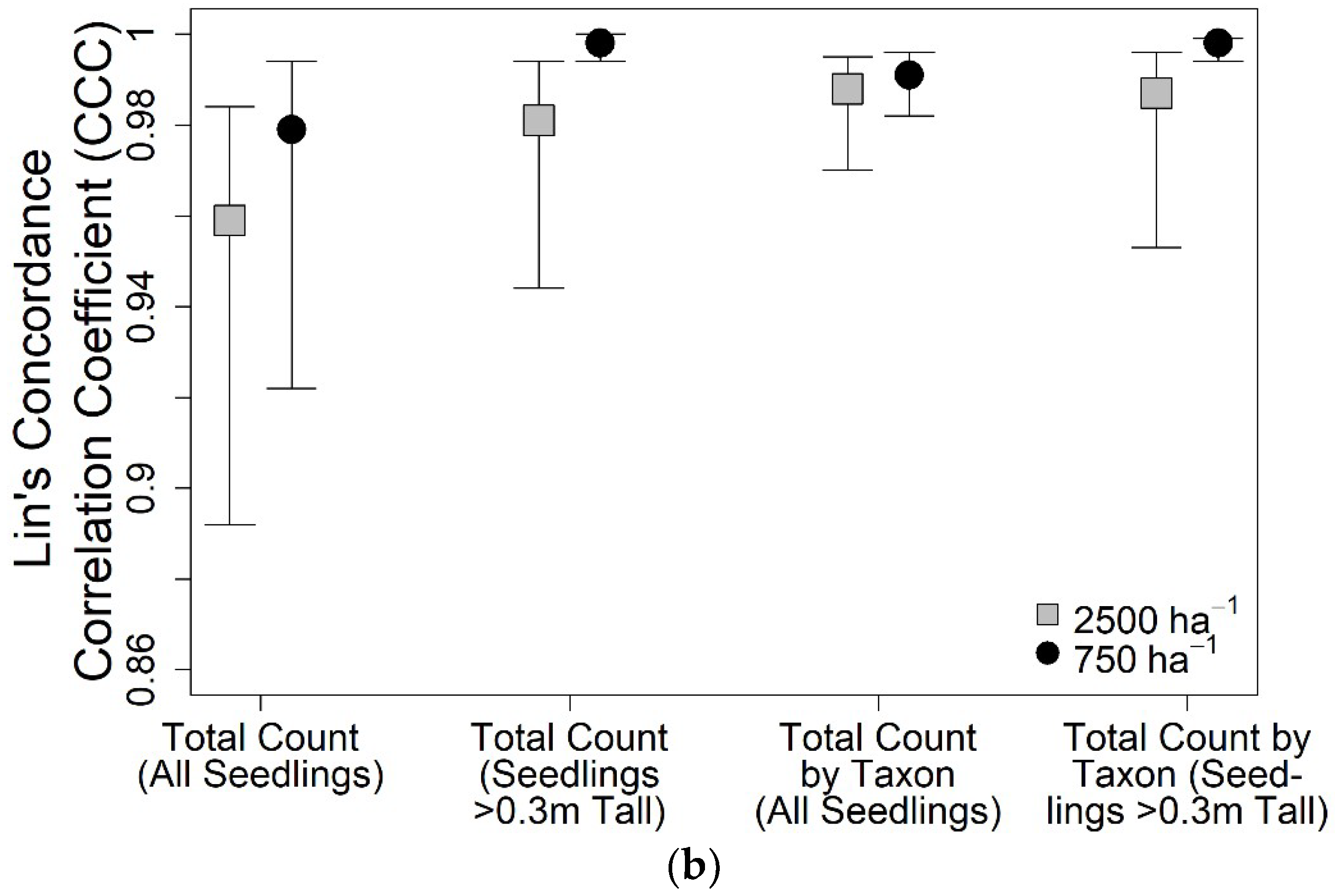
3. Results
4. Discussion
5. Conclusions
Author Contributions
Funding
Acknowledgments
Conflicts of Interest
Appendix A

| Common Name | Scientific Name |
|---|---|
| American basswood | Tilia americana L. |
| Bigtooth aspen | Populus grandidentata Michx. |
| Black ash | Fraxinus nigra Marshall |
| Black cherry | Prunus serotina Ehrh. |
| Black oak | Quercus velutina Lam. |
| Chestnut oak | Quercus montana Willd. |
| Cucumbertree | Magnolia acuminata L. |
| Green ash | Fraxinus pennsylvanica Marshall |
| Hemlock | Tsuga canadensis (L.) Carrière |
| Hickory (genus) | Carya spp. |
| Paper birch | Betula papyrifera Marshall |
| Pitch pine | Pinus rigida Mill. |
| Quaking aspen | Populus tremuloides Michx. |
| Red maple | Acer rubrum L. |
| Red oak | Quercus rubra L. |
| Scarlet oak | Quercus coccinea Münchh. |
| Sugar maple | Acer saccharum Marshall |
| White ash | Fraxinus americana L. |
| White oak | Quercus alba L. |
| White pine | Pinus strobus L. |
| Yellow birch | Betula alleghaniensis Britton |
| Yellow poplar | Liriodendron tulipifera L. |

References and Notes
- Lindenmayer, D.B.; Likens, G.E.; Andersen, A.; Bowman, D.; Bull, C.M.; Burns, E.; Dickman, C.R.; Hoffmann, A.A.; Keith, D.A.; Liddell, M.J.; et al. Value of long-term ecological studies. Austral Ecol. 2012, 37, 745–757. [Google Scholar] [CrossRef]
- Ravlin, F.W.; Voshell, J.R., Jr.; Smith, D.W.; Rutherford, S.L.; Hiner, S.W.; Haskell, D.A. Section I: Overview. In Shenandoah National Park Long-Term Ecological Monitoring System User Manuals; U.S. Department of the Interior, National Park Service: Washington, DC, USA, 1990; pp. I-1–I-17. [Google Scholar]
- Milberg, P.; Bergstedt, J.; Fridman, J.; Odell, G.; Westerberg, L. Observer bias and random variation in vegetation monitoring data. J. Veg. Sci. 2008, 19, 633–644. [Google Scholar] [CrossRef] [Green Version]
- Symstad, A.J.; Wienk, C.L.; Thorstenson, A.D. Precision, repeatability, and efficiency of two canopy-cover estimate methods in northern great plains vegetation. Rangel. Ecol. Manag. 2008, 61, 419–429. [Google Scholar] [CrossRef]
- Chandra Sekar, K.; Rawal, R.S.; Chaudhery, A.; Pandey, A.; Rawat, G.; Bajapai, O.; Joshi, B.; Bisht, K.; Mishra, B.M. First GLORIA site in Indian Himalayan region: Towards addressing issue of long-term data deficiency in the Himalaya. Natl. Acad. Sci. Lett. 2017, 40, 355–357. [Google Scholar] [CrossRef]
- Fleming, G.M.; Diffendorfer, J.E.; Zedler, P.H. The relative importance of disturbance and exotic-plant abundance in California coastal sage scrub. Ecol. Appl. 2009, 19, 2210–2227. [Google Scholar] [CrossRef] [PubMed]
- Li, S.; Pennings, S.C. Disturbance in Georgia salt marshes: Variation across space and time. Ecosphere 2016, 7, 1–11. [Google Scholar] [CrossRef]
- Van Lierop, P.; Lindquist, E.; Sathyapala, S.; Franceschini, G. Global forest area disturbance from fire, insect pests, diseases and severe weather events. For. Ecol. Manag. 2015, 352, 78–88. [Google Scholar] [CrossRef]
- Melillo, J.M.; Butler, S.; Johnson, J.; Mohan, J.; Steudler, P.; Lux, H.; Burrows, E.; Bowles, F.; Smith, R.; Scott, L.; et al. Soil warming, carbon-nitrogen interactions, and forest carbon budgets. Proc. Natl. Acad. Sci. USA 2011, 108, 9508–9512. [Google Scholar] [CrossRef] [PubMed] [Green Version]
- Mahan, C.G.; Diefenbach, D.R.; Cass, W.B. Evaluating and revising a long-term monitoring program for vascular plants: Lessons from Shenandoah National Park. Nat. Areas J. 2007, 27, 16–24. [Google Scholar] [CrossRef]
- Munson, S.M.; Duniway, M.C.; Johanson, J.K. Rangeland monitoring reveals long-term plant responses to precipitation and grazing at the landscape scale. Rangel. Ecol. Manag. 2016, 69, 76–83. [Google Scholar] [CrossRef]
- Bagchi, S.; Singh, N.J.; Briske, D.D.; Bestelmeyer, B.T.; McClaran, M.P.; Murthy, K. Quantifying long-term plant community dynamics with movement models: Implications for ecological resilience: Implications. Ecol. Appl. 2017, 27, 1514–1528. [Google Scholar] [CrossRef] [PubMed]
- Frerker, K.L.; Sabo, A.; Waller, D. Long-term regional shifts in plant community composition are largely explained by local deer impact experiments. PLoS ONE 2014, 9, e0185037. [Google Scholar] [CrossRef] [PubMed]
- Groffman, P.M.; Rustad, L.E.; Templer, P.H.; Campbell, J.L.; Lynn, M.; Lany, N.K.; Socci, A.M.; Vadeboncoeur, M.A.; Schaberg, P.G.; Wilson, F.; et al. Long-term integrated studies show complex and surprising effects of climate change in the northern hardwood forest. Bioscience 2012, 62, 1056–1066. [Google Scholar] [CrossRef]
- Liknes, G.C.; Nelson, M.D.; Kaisershot, D.J. Net Change in Forest Density, 1873–2001: Using Historical Maps to Monitor Long-Term Forest Trends; U.S. Department of Agriculture, Forest Service, Northern Research State: Newton Square, PA, USA, 2011; p. 12.
- Miles, P.D.; Brand, G.J.; Alerich, C.L.; Bednar, L.F.; Woudenberg, S.W.; Glover, J.F.; Ezzell, E.N. The Forest Inventory and Analysis Database: Database Description and Users Manual; version 1.0; U.S. Department of Agriculture, Forest Service, Northern Central Reseach Station: St. Paul, MN, USA, 2001.
- Goeking, S.A. Disentangling Forest change from forest inventory change: A case study from the US Interior West. J. For. 2015, 113, 475–483. [Google Scholar] [CrossRef]
- Morrison, L.W. Observer error in vegetation surveys: A review. J. Plant Ecol. 2016, 9, 367–379. [Google Scholar] [CrossRef]
- Bosworth, D. Forest Inventory and Analysis Strategic Plan; U.S. Department of Agriculture, Forest Service: Washington, DC, USA, 2007.
- U.S. Department of Agriculture, Forest Service, Northern Research Station. Forest Inventory and Analysis National Core Field Guide—Volume I Supplement: Field Data Collection Procedures For Phase 2+ Plots. Available online: https://www.nrs.fs.fed.us/fia/data-collection/field-guides/ver7.1/NRS%20FG%207.1-April%202017-Complete%20Document_NRSP2plus.pdf (accessed on 15 October 2018).
- Department of Conservation and Natural Resources Bureau of Forestry. Inventory Manual of Procedure for The 4th Cycle of CFI Measurements (2015–2020), Inventory of Biological Resources.
- U.S. Department of Agriculture, Forest Service. About the Agency: What We Believe. Available online: https://www.fs.fed.us/about-agency (accessed on 18 October 2018).
- Pennsylvania Department of Conservation and Natural Resources. DCNR Bureau of Forestry—Our Mission and What We Do. Available online: https://www.dcnr.pa.gov/about/Pages/Forestry.aspx (accessed on 18 October 2018).
- Albright, T.A.; McWilliams, W.H.; Widmann, R.H.; Butler, B.J.; Crocker, S.J.; Kurtz, C.M.; Lehman, S.L.; Lister, T.W.; Miles, P.D.; Morin, R.S.; et al. Pennsylvania Forests 2014; U.S. Department of Agriculture, Forest Service, Northern Research Station: Newton Square, PA, USA, 2017.
- Pennsylvania Department of Conservation and Natural Resources, Bureau of Forestry. Detecting & Monitoring Vegetation Changes within DMAP Units: Vegetation Impact Protocol in an Adaptive Resource Management Context.
- Pennsylvania—Department of Conservation and Natural Resource—Bureau of Forestry—Ecological Service. White-Tailed Deer Plan. Available online: http://www.docs.dcnr.pa.gov/cs/groups/public/documents/document/dcnr_20027101.pdf (accessed on 15 October 2018).
- Begley-Miller, D.R.; Hipp, A.L.; Brown, B.H.; Hahn, M.; Rooney, T.P. White-tailed deer are a biotic filter during community assembly, reducing species and phylogenetic diversity. AoB Plants 2014, 6, 1–9. [Google Scholar] [CrossRef] [PubMed]
- Rooney, T.P. High white-tailed deer densities benefit graminoids and contribute to biotic homogenization of forest ground-layer vegetation. Plant Ecol. 2009, 202, 103–111. [Google Scholar] [CrossRef]
- Côté, S.D.; Rooney, T.P.; Tremblay, J.-P.; Dussault, C.; Waller, D.M. Ecological impacts of deer overabundance. Annu. Rev. Ecol. Evol. Syst. 2004, 35, 113–147. [Google Scholar] [CrossRef]
- Habeck, C.W.; Schultz, A.K. Community-level impacts of white-tailed deer on understorey plants in North American forests: A meta-analysis. AoB Plants 2015, 7, plv119. [Google Scholar] [CrossRef] [PubMed]
- Tilghman, N.G. Impacts of white-tailed deer on forest regeneration in northwestern Pennsylvania. J. Wildl. Manag. 1989, 53, 524–532. [Google Scholar] [CrossRef]
- Horsley, S.B.; Stout, S.L.; DeCalesta, D.S. White-tailed deer impact on the vegetation dynamics of a northern hardwood forest. Ecol. Appl. 2003, 13, 98–118. [Google Scholar] [CrossRef]
- Rosenberry, C.S.; Fleegle, J.T.; Wallingford, B.D. Management and Biology of White-Tailed Deer in Pennsylvania 2009–2018; Pennsylvania Game Commission: Harrisburg, PA, USA, 2009. [Google Scholar]
- McCarthy, M.A.; Moore, J.L.; Morris, W.K.; Parris, K.M.; Garrard, G.E.; Vesk, P.A.; Rumpff, L.; Giljohann, K.M.; Camac, J.S.; Bau, S.S.; et al. The influence of abundance on detectability. Oikos 2013, 122, 717–726. [Google Scholar] [CrossRef]
- Müller, F.; Baessler, C.; Schubert, H.; Klotz, S. Long-Term Ecological Research: Between Theory and Application; Springer: Dordecht, The Netherlands, 2010; ISBN 9789048187812. [Google Scholar]
- Martínez-Abraín, A. Is the “n = 30 rule of thumb” of ecological field studies reliable? A call for greater attention to the variability in our data. Anim. Biodivers. Conserv. 2014, 37, 95–100. [Google Scholar]
- Russell, M.B.; Woodall, C.W.; Potter, K.M.; Walters, B.F.; Domke, G.M.; Oswalt, C.M. Interactions between white-tailed deer density and the composition of forest understories in the northern United States. For. Ecol. Manag. 2017, 384, 26–33. [Google Scholar] [CrossRef] [Green Version]
- Beardall, V.; Gill, R.M.A. The impact of deer on woodlands: The effects of browsing and seed dispersal on vegetation structure and composition. Forestry 2001, 74, 209–218. [Google Scholar]
- Frerker, K.L.; Sonnier, G.; Waller, D.M. Browsing rates and ratios provide reliable indices of ungulate impacts on forest plant communities. For. Ecol. Manag. 2013, 291, 55–64. [Google Scholar] [CrossRef]
- Waller, D.M.; Alverson, W.S. The White-tailed deer: A keystone herbivore. Wildl. Soc. Bull. 1997, 25, 217–226. [Google Scholar]
- National Oceanic and Atmospheric Administration. Normal Dates of Last Freeze in Spring and First Freeze in Autumn Across Central Pennsylvania. Available online: http://www.weather.gov/ctp/FrostFreeze (accessed on 1 January 2017).
- National Oceanic and Atmospheric Administration NOWData NOAA Data Online Weather Data. Available online: http://w2.weather.gov/climate/xmacis.php?wfo=ctp (accessed on 1 January 2017).
- Kirschbaum, C.D.; Anacker, B.L. The utility of Trillium and Maianthemum as phyto-indicators of deer impact in northwestern Pennsylvania, USA. For. Ecol. Manag. 2005, 217, 54–66. [Google Scholar] [CrossRef]
- Rooney, T.P.; Gross, K. A demographic study of deer browsing impacts on Trillium grandiflorum. Plant Ecol. 2003, 168, 267–277. [Google Scholar] [CrossRef]
- Royo, A.A.; Stout, S.L.; DeCalesta, D.S.; Pierson, T.G. Restoring forest herb communities through landscape-level deer herd reductions: Is recovery limited by legacy effects? Biol. Conserv. 2010, 143, 2425–2434. [Google Scholar] [CrossRef]
- Gamer, M.; Lemon, J.; Fellows, I.; Singh, P. Package ‘irr’: Various Coefficients of Interrater Reliability and Agreement. Available online: https://cran.r-project.org/web/packages/irr/irr.pdf (accessed on 15 October 2018).
- R Core Team. R: A Language and Environment for Statistical Computing. Available online: https://www.R-project.org (accessed on 15 October 2018).
- Mabmud, S.M. Cohen’s Kappa. In Encyclopedia of Research Design; Salkind, N., Ed.; SAGE Publications, Inc.: Thousand Oaks, CA, USA, 2012; pp. 188–189. ISBN 9781412961271. [Google Scholar]
- Landis, J.R.; Koch, G.G. The measurement of observer agreement for categorical data. Int. Biom. Soc. 1977, 33, 159–174. [Google Scholar] [CrossRef]
- Carrasco, J.L.; Martinez, J.P. Package ‘cccrm’: Concordance Correlation Coefficient for Repeated (and Non-Repeated) Measures. Available online: https://cran.r-project.org/web/packages/cccrm/cccrm.pdf (accessed on 15 October 2018).
- King, T.S.; Cinchilli, V.M.; Carrasco, J.L. A repeated measures concordance correlation coefficient. Stat. Med. 2007, 26, 3095–3113. [Google Scholar] [CrossRef] [PubMed]
- Lin, L.I.; McBride, G.; Bland, J.M.; Altman, D.G. A Proposal For Strength-Of-Agreement Criteria for Lin’S Concordance Correlation Coefficient; National Institute of Water & Atmopheric Research Ltd.: Hamilton, New Zealand, 2005. [Google Scholar]
- Zanarini, M.C.; Frankenburg, F.R.; Vujanovic, A. Inter-rater and test-retest reliability of the Revised Diagnostic Interview for Borderlines. J. Pers. Disord. 2002, 16, 270–276. [Google Scholar] [CrossRef] [PubMed]
- Awatani, T.; Morikita, I.; Shinohara, J.; Mori, S.; Nariai, M.; Tatsumi, Y.; Nagata, A.; Koshiba, H. Intra- and inter-rater reliability of isometric shoulder extensor and internal rotator strength measurements performed using a hand-held dynamometer. J. Phys. Ther. Sci. 2016, 28, 3054–3059. [Google Scholar] [CrossRef] [PubMed] [Green Version]
- Meeremans, P.; Yochum, N.; Kochzius, M.; Ampe, B.; Tuyttens, F.A.M.; Uhlmann, S.S. Inter-rater reliability of categorical versus continuous scoring of fish vitality: Does it affect the utility of the reflex action mortality predictor (RAMP) approach? PLoS ONE 2017, 12, e0179092. [Google Scholar] [CrossRef] [PubMed] [Green Version]
- Björk, J.; Rittner, R.; Cromley, E. Exploring inter-rater reliability and measurement properties of environmental ratings using kappa and colocation quotients. Environ. Health 2014, 13, 1–11. [Google Scholar] [CrossRef] [PubMed]
- Smith, S.D.; Charlet, T.N.; Zitzer, S.F.; Abella, S.R.; Vanier, C.H.; Huxman, T.E. Long-term response of a Mojave Desert winter annual plant community to a whole-ecosystem atmospheric CO2 manipulation (FACE). Glob. Chang. Biol. 2014, 20, 879–892. [Google Scholar] [CrossRef] [PubMed]
- Ritchie, M.E.; Tilman, D.; Knops, J.M.H. Herbivore effects on plant and nitrogen dynamics in oak savanna. Ecology 1998, 79, 165–177. [Google Scholar] [CrossRef]
- Morrissey, R.C.; Jacobs, D.F.; Seifert, J.R. Response of Northern Red Oak, Black Walnut, and White Ash Seedlings to Various Levels of Simulated Summer Deer Browsing; U.S. Department of Agriculture, Forest Service, Northern Research Station: Newtown Square, PA, USA, 2008; pp. 50–58.
- Augustine, D.J.; McNaughton, S.J. Ungulate effects on the functional species composition of plant communities: Herbivore selectivity and plant tolerance. J. Wildl. Manag. 1998, 62, 1165–1183. [Google Scholar] [CrossRef]
- Akobeng, A.K. Understanding type I and type II errors, statistical power and sample size. Acta Paediatr. 2016, 105, 605–609. [Google Scholar] [CrossRef] [PubMed]
- Zhang, J.; Nielsen, S.E.; Grainger, T.N.; Kohler, M.; Chipchar, T.; Farr, D.R. Sampling plant diversity and rarity at landscape scales: Importance of sampling time in species detectability. PLoS ONE 2014, 9. [Google Scholar] [CrossRef] [PubMed]
- Butt, N.; Slade, E.; Thompson, J.; Malhi, Y.; Riutta, T. Quantifying the sampling error in tree census measurements by volunteers and its effect on carbon stock estimates. Ecol. Appl. 2013, 23, 936–943. [Google Scholar] [CrossRef] [PubMed] [Green Version]
- Vittoz, P.; Guisan, A. How reliable is the monitoring of permanent vegetation plots? A test with multiple observers. J. Veg. Sci. 2017, 18, 413–422. [Google Scholar] [CrossRef]
- Wright, W.J.; Irvine, K.M.; Warren, J.M.; Barnett, J.K. Statistical design and analysis for plant cover studies with multiple sources of observation errors. Methods Ecol. Evol. 2017, 8, 1832–1841. [Google Scholar] [CrossRef]
- Mason, N.W.H.; Holdaway, R.J.; Richardson, S.J. Incorporating measurement error in testing for changes in biodiversity. Methods Ecol. Evol. 2018, 9, 1296–1307. [Google Scholar] [CrossRef]
- Otypková, Z.; Chytrý, M. Effects of plot size on the ordination of vegetation samples. J. Veg. Sci. 2006, 17, 465–472. [Google Scholar] [CrossRef]
- Bormann, F.H. The statistical efficience of the sample plot. Ecology 1953, 34, 474–487. [Google Scholar] [CrossRef]
- Dengler, J.; Löbel, S.; Dolnik, C. Species constancy depends on plot size—A problem for vegetation classification and how it can be solved. J. Veg. Sci. 2009, 20, 754–766. [Google Scholar] [CrossRef]
- Stohlgren, T.J.; Chong, G.W.; Kalkhan, M.A.; Schell, L.D.; Applications, S.E.; Aug, N. Multiscale Sampling of Plant Diversity: Effects of minimum mapping unit size. Ecol. Appl. 2014, 7, 1064–1074. [Google Scholar] [CrossRef]
- Johnson, S.E.; Mudrak, E.L.; Beever, E.A.; Sanders, S.; Waller, D.M. Comparing power among three sampling methods for monitoring forest vegetation. Can. J. For. Res. 2008, 38, 143–156. [Google Scholar] [CrossRef]
- Fike, J. (Ed.) Terrestrial & Palustrine Plant Communities of Pennsylvania; Pennsylvania Department of Conservation and Natural Resources: Harrisburg, PA, USA, 1999.


| Code | Definition |
|---|---|
| 1 | Very Low—Plot is inside a well-maintained deer exclosure. |
| 2 | Low—No browsing observed, vigorous seedlings present (no deer exclosure present). |
| 3 | Medium—Browsing evidence observed but not common, seedlings present. |
| 4 | High—Browsing evidence common OR seedlings are rare. |
| 5 | Very High—Browsing evidence omnipresent OR forest floor bare, severe browse line. |
This article is published under the terms of the free Open Government License, which permits unrestricted use, distribution and reproduction in any medium, provided the original author and source are credited: See: https://www.copyrightlaws.com/copyright-laws-in-u-s-government-works/.
Share and Cite
Begley-Miller, D.R.; Diefenbach, D.R.; McDill, M.E.; Rosenberry, C.S.; Just, E.H. Evaluating Inter-Rater Reliability and Statistical Power of Vegetation Measures Assessing Deer Impact. Forests 2018, 9, 669. https://doi.org/10.3390/f9110669
Begley-Miller DR, Diefenbach DR, McDill ME, Rosenberry CS, Just EH. Evaluating Inter-Rater Reliability and Statistical Power of Vegetation Measures Assessing Deer Impact. Forests. 2018; 9(11):669. https://doi.org/10.3390/f9110669
Chicago/Turabian StyleBegley-Miller, Danielle R., Duane R. Diefenbach, Marc E. McDill, Christopher S. Rosenberry, and Emily H. Just. 2018. "Evaluating Inter-Rater Reliability and Statistical Power of Vegetation Measures Assessing Deer Impact" Forests 9, no. 11: 669. https://doi.org/10.3390/f9110669