Article

Research on Energy Management Strategies of Extended-Range Electric Vehicles Based on Driving Characteristics

1
State Key Laboratory of Automotive Simulation and Control, Jilin University, Changchun 130022, Jilin, China
2
School of Mechanical and Aerospace Engineering, Jilin University, Changchun 130022, Jilin, China
*
Author to whom correspondence should be addressed.
World Electr. Veh. J. 2020, 11(3), 54; https://doi.org/10.3390/wevj11030054
Submission received: 12 June 2020 / Revised: 24 July 2020 / Accepted: 3 August 2020 / Published: 5 August 2020

Abstract

:
The extended-range electric vehicle (E-REV) can solve the problems of short driving range and long charging time of pure electric vehicles, but it is necessary to control the engine working points and allocate the power of the energy sources reasonably. In order to improve the fuel economy of the vehicle, an energy management strategy (EMS) that can adapt to the daily driving characteristics of the driver and adjust the control parameters online is proposed in this paper. Firstly, through principal component analysis (PCA) and iterative self-organizing data analysis techniques algorithm (ISODATA) of historical driving data, a typical driving cycle which can describe driving characteristics of the driver is constructed. Then offline optimization of control parameters by adaptive simulated annealing under each typical driving cycle and online recognition of driving cycles by extreme learning machine (ELM) are applied to the adaptive multi-workpoints energy management strategy (A-MEMS) of E-REV. In the end, compared with traditional rule-based control strategies, A-MEMS achieves good fuel-saving and emission-reduction result by simulation verification, and it explores a new and feasible solution for the continuous upgrade of the EMS.

Graphical Abstract

1. Introduction

In recent years, problems caused by energy shortage and environmental pollution are serious and need to be solved by energy-saving, emission-reduction and a low-carbon lifestyle. The hybrid electric vehicle is a transition model of a traditional internal combustion engine vehicle to a pure electric vehicle. After years of development, hybrid technology has become quite mature. Extended-range electric vehicle (E-REV), a type of hybrid electric vehicle, has an extra range extender, which includes an engine and a generator [1]. Since E-REV has two energy sources and each energy source has its own high-efficient range, the fuel-consumption performance of E-REV is sensitive to driving conditions [2]. In order to improve the vehicle economy and reduce emissions, its energy management strategy (EMS) needs to consider the real driving condition, and be constructed based on driving cycle recognition [3].
A driving cycle is a speed-time profile for a vehicle driving under a specified condition [4], usually represented by small fragments segmented from driving data, which are used as samples to build the driving condition database. Many researchers extracted different characteristics of the data to describe the driving cycle and attempted to reduce the dimension of feature vector [5,6,7]. Classical machine learning algorithm, like k-means [8], hidden Markov models [9], fuzzy c-means [10] is widely used in driving data analysis and driving cycle clustering. Recently with the development of deep learning, a neural network has been wildly applied in the field of pattern recognition and achieved good performances [11]. Lorenzo Berzi divided driving data into nine categories and built a GUI for generating driving cycle for electrical vehicles in the city of Florence according to different requirements [12]. Countries also have corresponding driving cycles for vehicle testing [4]. Donateo et al. [13] built a driving cycle for EU6d Emission Regulation and studied the effect of speed and acceleration on emission. In 2019, China Light-duty vehicles Test Cycle-Passenger (CLTC-P) were introduced [14,15].
In order to make the vehicle adapt to the complex and changeable driving conditions, the energy management problem of E-REV has attracted the attention of researchers in the past decade [16]. EMS can be divided into two categories: rule-based control and optimization-based control. Rule-based control includes thermostat control strategy, power following control strategy, and multi-workpoints control strategy [17], which build control rules by experiments and engineering experience. These strategies have a wide range of applications, but are poorly targeted.
The optimization-based energy management strategy is divided into global optimization and real-time optimization. Global optimization includes Dynamic Programming (DP) [18] and Pontryagin’s Minimum Principle (PMP) [19]. DP can obtain the multi-stage optimization decision under the situation where the global driving cycle is known, but its calculation is too difficult to be applied in real-time control. Meanwhile, the distribution of engine working points by DP is scattered, but most studies did not consider transient fuel consumption and its error with the steady-state fuel consumption model could reach 58% [20]. Therefore, single-point control is often used in practical applications, such as Nissan e-power [21] which can avoid the impact of transient fuel consumption. For real-time optimal control strategy, the equivalent consumption minimum strategy (ECMS) and model predictive control (MPC) are the two most common strategies. MPC predicts the power demand of the vehicle in the future by real-time driving data, and optimizes the power distribution ratio between engine and battery to achieve low fuel consumption [22]. ECMS minimizes the equivalent fuel consumption at each time which simplifies the dynamic optimization problem to an instantaneous optimization problem [23]. Nowadays, deep reinforcement learning (RL) has become a popular research topic [24,25,26]. Learning-based strategy has a good capability of generalization to complex driving conditions by continuous learning and achieves almost the same performance as DP. The proposed energy management strategy based on Deep Q-network in Ref [24] achieves 16.3% energy savings on a typical commute trip. However, though RL-based optimal and predictive control strategy is model-free, it is fully data-driven and needs a large number of training samples. Some EMS optimizes the control parameters offline by genetic algorithms (GA) [27] and simulated annealing (SA), which can also be applied in real-time control to improve the fuel economy. Lei optimized parameters of powertrain components and thermostat control strategy by simulated annealing particle swarm optimization under 23 typical driving cycles, and reduced the fuel consumption by 11.68% [28].
The optimization of control parameters based on driving cycle recognition is necessary for fuel economy [28]. However, the existing driving cycles are difficult to reflect personal driving characteristics and daily commute routes. Few papers analyzed how to optimize control parameters based on personal historical driving data. In this paper, ISODATA is used to cluster personal driving data to construct typical driving cycles for a specific driver, and the control parameters are optimized for each typical driving cycle by adaptive simulated annealing. In addition, the selection of control parameters is based on the engine multi-point control strategy, which can better adapt to different power requirements than the single-point control used in Nissan e-power [29].
The sections of this paper are organized as follows. In Section 2, constructing the typical driving cycle of a specific driver by data preprocessing, principal component analysis and clustering. In Section 3, establishing a novel energy management strategy by control parameter offline optimization under typical driving cycles and driving cycle online recognition. Meanwhile, the result of fuel consumption and emissions is verified by simulation compared with other control strategies, which is followed by the conclusion in Section 4.

2. Driving Cycles Clustering and Recognition

The real driving conditions are complex and changeable, in order to construct an effective EMS which can improve the fuel economy of an extended-range electric vehicle, it is necessary to construct typical driving cycles that can accurately and reliably characterize the driver’s driving condition [30].
As shown in Figure 1, the typical driving cycle construction method for a specific driver can be divided into following four steps:
  • Collection and preprocessing driver’s driving data.
  • Selection and principal component analysis of driving characteristics.
  • Cluster analysis and verification of driving characteristics.
  • Construction typical driving cycles for the driver.

2.1. Driving Data Preprocessing

In this work, the experimental vehicle is driven by a specific driver who basically follows a fixed commute route on weekdays. The vehicle is equipped with a Global Positioning System (GPS) receiver HOLUX RCV-3000 with MT3333 chipset and 4 MB flash memory for 250,000 log data recording such as speed, time, longitude, latitude and altitude. The acquisition time is 1 s. The collected real-time vehicle driving data was stored in the driving database and can be exported by its supporting software. However, errors will inevitably be encountered during the measurement process, thus the collected driving data needs to be preprocessed. The causes of errors include data loss, data anomalies and noise data.
The data loss due to discontinuity-time caused by a short-time failure of the GPS receiver can be complemented by interpolation; the data loss caused by factors such as long-term failure of the GPS or external building occlusion can be directly eliminated. Data anomalies commonly include speed or acceleration/deceleration anomalies, which can use linear interpolation to solve; and if it is the anomaly of latitude and longitude or long-term idle speed, it can be eliminated.
The acquired signal often contains noise. If these noise signals are not removed, the result may be affected or even the wrong conclusion may be drawn. Wavelet noise reduction uses wavelet transform to eliminate the noise contained in the original signal. It can not only effectively remove noise, but also retain the characteristics of the original signal to the greatest extent [31]. The application of wavelet analysis has been used not only in the field of mathematics, but also in the fields of signal analysis, image processing, medicine, and computers.
The vehicle speed data is a non-stationary random signal, which is a continuous quantity in time and amplitude [32]. Taking it at a certain time interval can obtain a series of one-dimensional discrete signals f ( t ) arranged in time, whose discrete wavelet transform is shown as Equation (1).
W f ( a , b ) = 2 a / 2 t = 0 N 1 f ( t ) ψ ^ ( t b 2 a ) ,
where a and b respectively represent the expansion factor and translation factor. ψ ^ is the fourier transform.
In order to realize finite discrete wavelet transform calculation, the numerical calculation often uses the multi-resolution signal decomposition algorithm proposed [33]. W f ( a , b ) can be represented as a pair of H = h k and G = g k filters ( k Z ) . h ˜ k and g ˜ k represent the corresponding image filter. If the discrete sampling signal of f ( t ) is expressed as { C ( n ) } , n is the sampling point. Driving speed time series v n ( 0 ) is regarded as the original signal of scale 0. Then the orthogonal wavelet decomposition can be written as Equations (2) and (3).
v j ( n ) = k Z h ˜ ( k 2 n ) v j 1 ( k )
D j ( n ) = k Z g ˜ ( k 2 n ) D j 1 ( k ) ,
where v j ( n ) and D j ( n ) are discrete approximation and discrete detail at 2 j resolution, which indicate the wavelet transform coefficient at this resolution. j = 0 , 1 , , J , J is the highest decomposition level.
Decompose the original signal v ( 0 ) into two parts, namely discrete approximation v ( 1 ) and discrete detail D ( 1 ) , and then further decompose the discrete approximation signal to obtain the decomposition results { v ( J ) , D ( J ) , D ( J 1 ) , , D ( 1 ) } . The threshold of wavelet transform changes with the decomposing scale. We retain the detail with absolute values greater than or equal to the threshold at each scale. Conversely, due to the orthogonality of the decomposition, the original signal v ( 0 ) can be reconstructed from { v ( J ) , D ( 1 ) , D ( 2 ) , , D ( J ) } shown as Equation (4).
v j 1 ( n ) = k Z h ( n 2 k ) v j ( k ) + k Z g ( n 2 k ) D j ( k ) .
According to the above principle, the vehicle speed signal, denoised by wavelet, can be obtained. Common indexes for evaluating the effect of wavelet denoising include root mean square error (MSE), signal-to-noise ratio (SNR) and smoothness [34]. MSE reflects the similarity between the original signal and the denoised signal. The smaller value of MSE, the more the original signal information is retained.
M S E = 1 n i = 1 n ( v ( i ) v ^ ( i ) ) 2 ,
where v ( i ) is the original signal and v ^ ( i ) is the denoised signal. n is the length of the signal.
SNR is the ratio of the signal energy to the noise energy. The greater value of SNR, the better the denoising effect.
S N R = 10 · lg ( i = 1 n ( v ( i ) 2 / i = 1 n ( v ( i ) v ^ ( i ) ) 2 ) .
Smoothness is an important indicator to judge the effect of abnormal data processing. The smaller the smoothness, the better the effect of abnormal data processing.
S m o o t h n e s s = i = 1 n 1 ( v ^ ( i + 1 ) v ^ ( i ) ) 2 / i = 1 n 1 ( v ( i + 1 ) v ( i ) ) 2 .
The daubechies wavelets at different scales are used to decompose the driving data. The SNR, MSE and smoothness at each decomposition scale are shown in Table 1. It can be seen from the table that the MSE is greatly increased and the SNR is greatly reduced at the seven-scale. Therefore, in order to make the obtained speed signal smoother while ensuring a better denoising effect, the decomposition scale is chosen to be 6.
Db wavelet and six-decomposition scale are used to perform wavelet denoising on the collected vehicle speed data. The vehicle speed and acceleration before and after noise reduction are shown in Figure 2. It can be seen from the figure that the speed and acceleration curve of the vehicle after wavelet denoising is smoother than before and the frequent fluctuation is reduced, which is more in line with the actual situation. That means the ideal denoising effect is obtained by using wavelet denoising.
Meanwhile, the power spectral density of the original vehicle speed signal and denoising signal is shown in Figure 3. The power spectrum of original speed signal has large fluctuations in the high-frequency phase, indicating that there is noise in the signal. After wavelet denoising, the fluctuation of power spectrum decreases after 0.2 Hz, and the power spectrum tends to zero after 0.4 Hz. In the low-frequency phase, the power spectrum is basically consistent with the original signal, indicating that the information of the signal is better-remained without distortion.

2.2. Characteristics Selection and Principal Component Analysis

This paper divides the collected driving data into short fragments, called kinematics sequences, and extracts the characteristics from each fragment. The kinematics sequences means the vehicle speed interval from the start of the idling state to the start of the next idling state, including the idling segment, acceleration segment, deceleration segment and even speed segment. Through the extraction and analysis of a large number of kinematics sequences, the daily driving law of the driver can be obtained, and optimizing the energy management strategy according to this law can improve the fuel economy and the emission.
A total of 1562 kinematics sequences are extracted from the historical driving database. The 21 characteristics in the Table 2 have different characterization capabilities for these fragments. Among them, the acceleration phase in this paper refers to the process of vehicle acceleration greater than 0.14 m / s 2 , and the deceleration phase refers to the process of vehicle deceleration greater than 0.14 m / s 2 . The even speed phase refers to the process where the vehicle speed is not zero and the acceleration and deceleration are both less than 0.14 m / s 2 , and the idle speed phase refers to the vehicle speed is zero.
Under the premise of ensuring that the driving information contained in kinematics sequences is basically unchanged, screening the characteristics in Table 2 can reduce the amount of calculation and eliminate the mutual interference between the characteristics. Meanwhile, it will improve the accuracy of the cluster analysis, and ultimately construct a reasonable driving cycle for the specific driver.
The correlation coefficient method is applied to solve the correlation between each characteristic of driving cycles and the correlation between the characteristics and the fuel consumption of the vehicle which will be used as the basis for screening. The correlation coefficient is determined by Equation (8).
R c o r = i = 1 n ( x i x ¯ ) ( y i y ¯ ) i = 1 n ( x i x ¯ ) 2 i = 1 n ( y i y ¯ ) 2 ,
where x i and y i are the i-th sample in two characteristics. x ¯ and y ¯ are the average value of the two characteristics respectively.
The correlation coefficient between the characteristics of driving cycles and the correlation between the characteristics and the fuel consumption of the vehicle is shown in Figure 4. It is worth pointing out that the self-correlation coefficient of each characteristic is 1. Comprehensively considering the influence of characteristics on fuel consumption and the correlation between characteristics, 13 characteristics of driving cycles are obtained after screening.
The 13 characteristics such as the average speed, the maximum speed and the standard deviation of the vehicle speed are represented by x 1 , x 2 , ⋯, x 13 . Characteristics of 1562 kinematics sequences are represented by matrix A = ( a i j ) 1562 × 13 . i is the index of kinematics sequences. [ a i 1 , a i 2 , , a i 13 ] is the characteristics of i-th kinematics sequences. However, if clustering analysis is carried out directly, the amount of calculation is large due to matrix A = ( a i j ) 1562 × 13 is huge. Principal Component Analysis (PCA) method can be used to reduce the dimension of feature vectors which can retain the original information to the greatest extent [35].
Figure 5 shows the variance contribution rate of each principal component and the cumulative variance contribution rate. It can be seen that the cumulative variance contribution rate of the first four principal components is 89.41%. The cumulative variance contribution rate of the first four principal components exceeds 85%, indicating that they contain most of the original driving data information [1]. That means after PCA, the dimension of the characteristics is further reduced from 13 to 4, which achieves the purpose of reducing the amount of calculation and lays the foundation for the subsequent cluster analysis.
The linear combination coefficients of the first to fourth principal component eigenvectors are shown in the Figure 6.

2.3. Cluster Analysis of Driving Cycle

Four principal components obtained after dimensionality reduction are used as the parameters reflecting the kinematics sequences. Next, the kinematics sequences need to be clustered to obtain several typical driving cycles for the driver, which is convenient for subsequent simulation analysis of fuel economy. Clustering is to divide the sample set into different categories according to a criterion. The purpose is to divide the samples with greater similarity into one category, and the similarity between different categories is as small as possible [36]. Common criteria are based on the distance between samples, that is, the smaller distance is divided into the same category, and the larger distance is divided into different categories. Euclidean distance is the most widely used method to measure the distance between samples. Therefore, this paper select Euclidean distance to calculate the distance between samples. The expression of Euclidean distance between two vectors is as shown in Equation (9).
d x y = i = 1 n ( x i y i ) 2 .
The K-means clustering method is a fast, simple and effective clustering algorithm, so it is often used in cluster analysis. The parameter k in the K-means algorithm represents the number of categories to be divided and is determined by man. Different classification numbers k may lead to completely different results. The brief flow of the K-means algorithm is shown as Table 3.
The K-means algorithm is suitable for data whose category number has been determined. For clustering data with unknown categories number and high dimensions, Iterative Self-Organizing Data Analysis Techniques Algorithm (ISODATA) can be considered. The ISODATA algorithm is an improved K-means algorithm which does not need to manually determine the number of categories [37]. The flow of ISODATA is shown in the Figure 7.
The ISODATA clustering algorithm introduces man–machine dialogue links by setting initial parameters, and uses mechanisms such as merging and splitting. When the center distance between two clusters is less than a certain threshold, they are merged into one class. When the standard deviation of a certain type is greater than a certain threshold or when the number of samples exceeds a certain threshold, it is split into two types, and when the number of samples of a certain type is less than a certain threshold, it is cancelled. In this way, iterate according to the parameters such as the initial clustering center and the threshold, and finally obtain an ideal clustering result.
K-means and the ISODATA method were respectively used to cluster the driving cycle data. Clustering effect was evaluated using indicators such as the silhouette coefficient, Calinski–Harabaz index (CH), and Davies–Bouldin index (DBI) which are applied when the actual category information is unknown.
If the silhouette coefficient, whose range is [−1, 1], is close to 1, it means that the clustering effect is good. A large value of CH means the samples in the sample category are more concentrated, and the distance between different categories is larger. The DBI is the average level that measures the maximum similarity of each clustering result. The smaller the value is, the greater the similarity among samples in the same category is, and the clustering effect is better.
As is shown in Table 4, silhouette coefficient and CH indexes of ISODATA method are the highest, and the index of DBI is just higher than K-means with three categories, which means that the clustering effect of ISODATA is better than K-means algorithms. As is shown in Figure 8, except for a small number of samples in the first and fifth categories whose silhouette coefficients are less than 0, the silhouette coefficients of other samples are relatively large. That also means ISODATA clustering is reasonable.
Based on the first four principal components mentioned above, the distribution of the clustering samples using ISODATA in the principal components space is shown in Figure 9. It can be seen from the figure that the samples are divided into five categories and boundary separation between the various types is obvious.
Select the kinematics fragment closest to the cluster center in each category as the typical driving cycle, shown in Figure 10. It can be seen from the figure that the difference between cycles is large, indicating that the clustering effect is good.
The characteristics value of five typical driving conditions is shown in Table 5, the meaning of the corresponding characteristic number is shown in Table 2. The collected data is the daily driving route of a driver in the urban area, so there is no high-speed section. Types 1 and 2 are urban congested road sections, with a frequent start and stop and low average speed. Type 2 congestion is more serious, and the proportion of 0–20 km/h reaches 75%. Type 5 is a relatively smooth section of the urban area. Types 3 and 4 are the city expressways where the maximum speed exceeds 60 km/h. Type 4 has an even speed for a long time, and the average speed is high, indicating the road condition is smooth.
Moreover, to further illustrate that the typical driving cycles constructed in this paper are more suitable for the collected driving data than existing driving cycles, like CLTC-P, WLTC and NEDC. The probability density function of each phase (idle, even speed, acceleration and deceleration) and speed in each driving cycle, and a scatter plot of average speed and idle speed time ratio are shown in Figure 11.
As is shown in Figure 11, the four phases of CLTC-P are approximately equal, which is more similar to the collected driving data than NEDC and WLTC. However, the speed of the high-speed section in CLTC-P is too high, which does not meet the driving conditions in the urban area. This also shows that the driving cycle can better reflect the driving characteristics of most drivers in a certain area, but lack of pertinence. So compared with the existing driving cycles, the probability density function of typical driving cycle constructed for the specific driver is similar to the collected driving data, and can reflect the daily driving condition and driving characteristics. There are still some differences between the two mainly because some kinematics fragments are not well classified whose silhouette coefficients are less than 0 in Figure 8. In Figure 11c, it can also be seen that the five typical driving cycle is different from existing driving cycles in average speed and idle speed time ratio.

2.4. Driving Condition Recognition Based on Extreme Learning Machine

The driving cycle recognition is to analyze the characteristics of the kinematics sequences and compare it with the characteristics of the known driving cycles, so as to identify the driving cycle of the vehicle. Extreme Learning Machine (ELM) is a new algorithm produced for the shortcomings of the single hidden layer feedforward neural network algorithm, which has the advantages of better generalization performance and faster learning speed [38]. The algorithm randomly generates the threshold of the hidden neuron and the connection weight between the input layer and the hidden layer, and does not need to be adjusted during the training process, only needs to set the number of hidden layer neurons. This work will use ELM to recognize driving cycles.
The network structure of the ELM, which is similar to the traditional BP neural network, includes three layers: the input layer, the hidden layer, and the output layer shown in the Figure 12. Each neuron in the input layer represents the characteristics used for driving cycle recognition. The hidden layer has only a single layer whose number of neurons can be adjusted. The number of neurons in the output layer is the only one whose output value is equal to the type of typical driving cycle.
The input sample set of the extreme learning machine is X = [ x 1 , x 2 , . . . , x N ] , N is the number of samples of driving cycle. x = [ x 1 , x 2 , x 3 , x 4 ] is the sample feature vector whose dimension is equal to the number of principal components obtained above, used for driving condition recognition. Therefore, the number of neurons in the input layer is also four.
Then if there are M neurons in the hidden layer, the output of the hidden layer of the ELM can be expressed as Equation (10).
H = g ( ω 1 · x 1 + b 1 ) g ( ω M · x 1 + b l ) g ( ω 1 · x N + b 1 ) g ( ω M · x N + b l ) N × M ,
where ω j = [ ω j , ω j 1 , ω j 2 , ω j 4 ] is the weight and b j is the bias of the j-th hidden layer neuron. g ( x ) is the activation function of hidden layer neurons, selecting Sigmoid function in this work.
The output of the output layer can be expressed as Equation (11). β j is the the weight between the output layer neuron of ELM and the j-th hidden layer neuron.
o = j = 1 l β j g ( ω j · x i + b j ) ,
when learning using ELM, if the activation function g ( x ) is infinitely differentiable, the parameters of the network do not need to be adjusted, ω and b are randomly generated during the training process, and remain unchanged during the training process. The weight β between the hidden layer and the output layer is obtained by solving the least square solution of the equation, shown as Equation (12)
min β H β T
The solution β ^ is shown as Equation (13).
β ^ = H + T ,
where H + is the generalized inverse matrix of the hidden layer output matrix H. T is the expected output of the network, which is the result of the above clustering.
The driving cycle samples obtained by clustering are divided into a training set and a test set with a 7:3 ratio, and each sample includes four principal component and the label of typical driving cycle type. By calculating the error between the predicted value and the expected value of the sample set, the generalization performance of the network is evaluated.
The hidden layer with different numbers of neural nodes obtains different result. It is necessary to select the appropriate number of nodes according to actual needs. The total recognition rate including training set and test set obtained by different numbers of neurons is shown in Figure 13. When the number of hidden layer nodes is 80, the recognition rate reaches 91.3%, which meets actual requirements, and also verifies that the characteristics do not lose the main information of the driving cycle data. When the number of nodes continues to increase, the recognition rate does not increase significantly, so 80 hidden layer nodes are selected for driving cycle recognition.

3. Energy Management Strategy for E-REV Based on Driving Characteristics

This section proposes an optimized energy management strategy of the E-REV based on driving characteristics. AVL Cruise is used to establish the vehicle model of E-REV and energy management strategy. With the goal of minimum energy consumption and emissions, off-line optimization calculation is performed for the five typical driving conditions selected above. Then the extreme learning machine is used to classify the actual driving cycles into five typical driving conditions, and the off-line optimization results are used for real-time energy management. Compared with the results of traditional energy management strategies, analyzing the energy-saving effect of this optimized energy management strategy.

3.1. Multi-Objective Optimization for Typical Driving Conditions

The basic parameters of the E-REV built in this paper shown in Table 6. According to the engine test data, the engine external characteristic curve and the brake specific fuel consumption (BSFC) map is shown in Figure 14a. Figure 14b is the efficiency map and maximum torque curve of the motor.
Common rule-based EMS of E-REV includes the thermostat control strategy, power following control strategy, and multi-workpoints control strategy.
  • Thermostat control: when the State of Charge (SOC) of battery is between S O C m i n and S O C m a x , the engine maintains the working state; when S O C is more than S O C m a x , the engine is turned off and runs on pure electric power; when SOC is less than S O C m i n , the engine works at the highest efficiency point, and the excess energy charges the battery. This strategy can effectively avoid engine start and stop frequently, but batteries often charge and discharge with a large current which is extremely bad for battery life.
  • Power following control: this strategy determines the working state of the engine according to the power demand of the vehicle and SOC of the battery. Only when SOC more than S O C m a x and the power demand is less than P e l o w , the engine will turn off. Under this control strategy, the battery can maintain the best performance state, but frequent engine fluctuations are detrimental to the economy and fuel consumption.
  • Multi-workpoints control: the strategy is to make the engine work at different working points according to the vehicle’s power demand and battery SOC. Too many working points will cause the engine fluctuation to become larger, and too few working points will not avoid the power battery work with large current. This strategy can not only ensure the life of the power battery but also reduce the fluctuation of the engine.
The dynamics, economy, and emissions of the vehicle are important performance indexes for evaluating EMS, but they are contradictory. Therefore, the optimization of EMS for E-REV is not a simple single-objective optimization problem, but a multi-objective optimization problem.
The simulated annealing algorithm is a heuristic search algorithm, which simulates the solid annealing process. Ingber [39] improved simulated annealing algorithm and proposed an adaptive simulated annealing (ASA) algorithm, which improved the performance and calculation speed of the algorithm. In this paper, the ASA is selected to optimize the control parameters of the EMS.
In the ASA algorithm, the solution m n + 1 s generated at the ( n + 1 ) -th iteration is shown in Equation (14), s is the s-th term of the solution vector.
m n + 1 s = m n s + y s ( B s A s ) ,
where B s , A s are the upper and lower limits of m s . y s can be calculated as Equation (15) and u s obeys uniform distribution on [0, 1].
y s = sgn ( u s 0.5 ) T s [ ( 1 + 1 / T s ) 2 u s 1 1 ] .
The feature of using this method to generate new solutions is that the search interval is large when the temperature is high, and the search interval is small when the temperature is low, which greatly improves the speed of the algorithm to search for the optimal solution.
Cooling function in adaptive simulated annealing algorithm is shown in Equation (16). T k is the temperature at the k-th iteration of the outer loop and T k is the initial temperature. S is the dimension of solution vector and C is a constant.
T k = T 0 exp ( C k 1 / S )
The greater the initial temperature or the greater the number of iterations is, the higher the probability of obtaining the optimal solution is, but the longer the calculation time requires. Therefore, the choice of initial temperature and iteration number needs to balance both optimization time and optimization effect. The flow of ASA is shown in Figure 15.
This work selects control parameters in multi-workpoints control strategy with three working speed of the engine to optimize, which switch according to the battery SOC and the vehicle speed. Then, the control parameters selected for optimization and their upper and lower limits are shown in Table 7.
Economy is one of the most important indexes to measure the performance of the vehicle. The economic evaluation parameters are commonly used for fuel consumption per hundred kilometers. Compared with traditional internal combustion engine vehicles, E-REV has an additional energy source from the battery. The conversion relationship between the fuel consumption per hundred kilometers of the extended-range engine and the battery consumption per hundred kilometers is shown in Equation (17).
Q e = E · 3600 ρ · q · η e · η g ,
where Q e represents the fuel consumption per hundred kilometers after equivalent conversion, the unit is L . E represents power consumption per hundred kilometers, the unit is kWh . ρ is the fuel density, the unit is g / cm 3 . q is the calorific value of fuel in J/g. η e and η g represent the average efficiency of the engine and generator, respectively.
The purpose of this work is to improve the economy and emissions of E-REV. The economic evaluation indexes include fuel consumption and electricity consumption per hundred kilometers. Emissions include nitrogen oxides, CO, and hydrocarbons. So the objective function is shown as Equation (18).
J = ω 1 Q f + ω 2 Q e + ω 3 E N O X + ω 4 E C O + ω 5 E H C ,
where Q f and Q e represent fuel consumption and electricity consumption per hundred kilometers. E N O X , E C O and E H C represent emissions of nitrogen oxides, CO, and hydrocarbons. [ ω 1 , ω 2 , ω 3 , ω 4 , ω 5 ] respectively represent the weight values of fuel consumption, electricity consumption and emissions, which can be determined according to actual requirement. In this paper, weight is selected as [0.35, 0.35, 0.1, 0.1, 0.1].
At the same time, in order to ensure the dynamics of the vehicle, dynamic constraints are shown in Table 8 need to be added.
The five typical driving cycles constructed above are imported into AVL Cruise software respectively, and optimized by the ASA algorithm. Figure 16 shows the iterative optimization process of some control parameters, including low, middle and high engine working speed, under the Type 2 typical driving cycle. It can be seen from the figure that after 100 iterations, the parameters have stabilized.
The optimization results of control parameters obtained by the ASA algorithm for five types of typical driving cycles are shown in Table 9. It can be seen from the table that the optimal control parameters under different driving cycles are quite different, which also shows the necessity of control parameter optimization.

3.2. Real-Time Energy Management Strategy Based on Driving Cycle Recognition

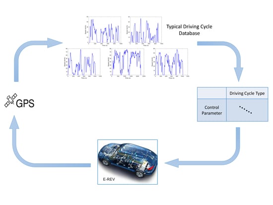
The control parameters of five typical working conditions have been optimized by ASA algorithm. However, the actual driving conditions of the vehicle are various. In order to let E-REV adapt to complex driving conditions and achieve the purpose of improving the fuel economy and emissions of the vehicle, an adaptive multi-workpoint energy management strategy based on offline parameter optimization and online driving cycle recognition (A-MEMS) has been proposed. Its control principle diagram is shown in Figure 17.
The actual driving condition needs to be divided into driving fragments for recognition according to a fixed step size, and the step length of the driving cycle recognition is selected to be 100 s. The characteristics in each step length are calculated separately, and principal components composed of these characteristics are input to the trained ELM. Select a section of actual driving condition, whose cycle time is 2100 s and total mileage is 19.73 km. The final recognition result of ELM is shown in Figure 18.
Respectively, simulation with three common rule-based energy management strategies including thermostat control strategy, power following control strategy, and multi-workpoints control strategy, and A-MEMS based on driving cycle recognition. There is only one engine workpoint in thermostat control, which works or not depending on SOC. The distributions of engine working points of the other three strategies are shown in the Figure 19.
During thermostat control, the working point is set in the high-efficiency zone and the engine power is selected to be 37.5 kW with a target speed of 4000 rpm and a target torque of 90 Nm. As is shown in Figure 19, working points of the power following strategy are concentrated near the minimum fuel consumption curve. The engine works at certain specified speeds of the multi-workpoints and A-MEMS. Compared with multi-workpoints control, the engine working range of low and medium speeds in A-MEMS has expanded, while the high-speed working range has slightly reduced. Meanwhile, working points of the engine in the optimized control are more biased towards the low fuel consumption area.
The A-MEMS categorizes actual driving fragments into the five typical driving cycles. It can be seen in Figure 20 that SOC limit of A-MEMS varies with driving cycle type. In 150–200 s, the recognition result is Type 2 where the vehicle speed fluctuates greatly and the average vehicle speed is low. Then, the upper limit of SOC is increased to improve the engine load, which means that the engine will work in a higher efficient region. Each driving cycle has its own optimal working speed of engine and limit of SOC, which can make engine mainly work at high-efficiency area with low and medium speed.
The equivalent fuel consumption per hundred kilometers, emissions and dynamics of the four energy management strategies are shown in Table 10. Compared with the other two rule-based control strategies, the multi-workpoints control strategy has lower fuel consumption and emissions. Under the power-following control strategy, although the engine works on the minimum fuel consumption curve, the engine runs for a long time, and the engine’s working state changes frequently, so the fuel consumption is greater than other strategies.
The equivalent fuel consumption of the A-MEMS based on driving cycle recognition is 8.9% lower than multi-workpoints control without driving cycle recognition, and 17.6% lower than that of the thermostat control strategy. The emissions of HC compounds, carbon monoxide, and nitrogen oxides in the exhaust gas were also reduced by 7.9%, 14.0%, and 13.4%, respectively, compared with multi-workpoints control, although the dynamics have been reduced slightly, though they still meet vehicle dynamic targets.

4. Conclusions

In this paper, an energy management strategy of E-REV that can adapt to the daily driving characteristics of the driver and adjust the control parameters online is proposed. To this end, we preprocess historical driving data by wavelet decomposition, and construct five typical driving cycles for the driver by PCA and ISODATA clustering. Then, control parameters of multi-workpoints control strategy in each typical driving cycle are optimized by ASA. Finally, combining online driving cycle recognition by ELM, the fuel-saving effect of the A-MEMS proposed in this paper is verified by simulation. Compared with traditional rule-based control strategies, A-MEMS achieve good fuel economy and reduce emissions, the average fuel saving is 9%–17%. In future research, the control strategy will be applied in the real vehicle by continuously recording driving data and regularly updating the control parameters in the ECU to verify the performance.

Author Contributions

Conceptualization, P.W.; investigation, Z.M.; methodology, P.W.; software, J.J.; writing—original draft, W.S.; writing—review and editing, Y.Y. All authors have read and agreed to the published version of the manuscript.

Funding

This research was supported by the National Key R&D Program of China (2018YFB0106200) and Natural Science Foundation of China (Grant no.51775229).

Conflicts of Interest

The authors declare no conflict of interest.

Abbreviations

The following abbreviations are used in this manuscript:
E-REVExtended-Range Electric Vehicle
EMSEnergy Management Strategy
CLTC-PChina Light-duty vehicles Test Cycle-Passenger
GPSGlobal Positioning System
MSEMean Square Error
SNRSignal-to-Noise Ratio
PCAPrincipal Component Analysis
ISODATAIterative Self-Organizing Data Analysis Techniques Algorithm
CHCalinski-Harabaz index
DBIDavies-Bouldin index
ELMExtreme Learning Machine
SOCState of Charge
ASAAdaptive Simulated Annealing
A-MEMSAdaptive Multi-workpoints Energy Management Strategy

References

  1. Xie, H.; Tian, G.; Chen, H.; Wang, J.; Huang, Y. A distribution density-based methodology for driving data cluster analysis: A case study for an extended-range electric city bus. Pattern Recognit. 2018, 73, 131–143. [Google Scholar] [CrossRef]
  2. Chrenko, D.; Gan, S.; Gutenkunst, C.; Kriesten, R.; Moyne, L.L. Novel Classification of Control Strategies for Hybrid Electric Vehicles. In Proceedings of the 2015 IEEE Vehicle Power and Propulsion Conference (VPPC), Montreal, QC, Canada, 19–22 October 2015; pp. 1–6. [Google Scholar]
  3. Yang, Y.; Zhang, Y.; Tian, J.; Li, T. Adaptive real-time optimal energy management strategy for extender range electric vehicle. Energy 2020, 197, 117237. [Google Scholar] [CrossRef]
  4. Tong, H.Y.; Hung, W.T. A Framework for Developing Driving Cycles with On-Road Driving Data. Transp. Rev. 2010, 30, 589–615. [Google Scholar] [CrossRef]
  5. Fotouhi, A.; Yusof, R.; Rahmani, R.; Mekhilef, S.; Shateri, N. A review on the applications of driving data and traffic information for vehicles’ energy conservation. Renew. Sustain. Energy Rev. 2014, 37, 822–833. [Google Scholar] [CrossRef]
  6. Shi, Q.; Zheng, Y.; Wang, R.; Li, Y. The study of a new method of driving cycles construction. Procedia Eng. 2011, 16, 79–87. [Google Scholar] [CrossRef] [Green Version]
  7. Ashtari, A.; Bibeau, E.; Shahidinejad, S. Using Large Driving Record Samples and a Stochastic Approach for Real-World Driving Cycle Construction: Winnipeg Driving Cycle. Transp. Sci. 2014, 48, 170–183. [Google Scholar] [CrossRef]
  8. Si, L.; Hirz, M.; Brunner, H. Big Data-Based Driving Pattern Clustering and Evaluation in Combination with Driving Circumstances; SAE Technical Papers; SAE International: Warrendale, PA, USA, 2018. [Google Scholar]
  9. Lee, J.; Li, J.; Liu, L.; Chen, C. A Novel Driving Pattern Recognition and Status Monitoring System; Lecture Notes in Computer Science; Springer: Berlin/Heidelberg, Germany, 2006; pp. 504–512. [Google Scholar]
  10. Yu, H.; Tseng, F.; Mcgee, R.A. Driving pattern identification for EV range estimation. In Proceedings of the 2012 IEEE International Electric Vehicle Conference, Greenville, SC, USA, 4–8 March 2012; pp. 1–7. [Google Scholar]
  11. Xie, L.; Tao, J.; Zhang, Q.; Zhou, H. CNN and KPCA-Based Automated Feature Extraction for Real Time Driving Pattern Recognition. IEEE Access 2019, 7, 123765–123775. [Google Scholar] [CrossRef]
  12. Berzi, L.; Delogu, M.; Pierini, M. Development of driving cycles for electric vehicles in the context of the city of Florence. Transp. Res. Part D Transp. Environ. 2016, 47, 299–322. [Google Scholar] [CrossRef]
  13. Donateo, T.; Giovinazzi, M. Building a cycle for Real Driving Emissions. Energy Procedia 2017, 126, 891–898. [Google Scholar] [CrossRef]
  14. China Automotive Driving Cycle-Part1: Light-Duty Vehicles, GB/T 38146.1-2019; National Technical Committee of Auto Standardization: Tianjin, China, 2019. (In Chinese)
  15. Zhang, J.; Yang, Y.; Zhou, Y. Parameter closed-loop optimization for pure electric vehicles unified design of power system and control parameters. J. Braz. Soc. Mech. Sci. Eng. 2020, 42, 229. [Google Scholar] [CrossRef]
  16. Zhang, F.; Hu, X.; Langari, R.; Cao, D. Energy management strategies of connected HEVs and PHEVs: Recent progress and outlook. Prog. Energy Combust. Sci. 2019, 73, 235–256. [Google Scholar] [CrossRef]
  17. Kopczyński, A.; Krawczyk, P.; Lasocki, J. Parameters selection of extended-range electric vehicle supplied with alternative fuel. E3S Web Conf. 2018, 44, 00073. [Google Scholar] [CrossRef] [Green Version]
  18. Romaus, C.; Gathmann, K.; Bocker, J. Optimal energy management for a hybrid energy storage system for electric vehicles based on Stochastic Dynamic Programming. In Proceedings of the 2010 IEEE Vehicle Power and Propulsion Conference, Lille, France, 1–3 September 2010; pp. 1–6. [Google Scholar]
  19. Xie, S.; Li, H.; Xin, Z.; Liu, T.; Wei, L. A Pontryagin Minimum Principle-Based Adaptive Equivalent Consumption Minimum Strategy for a Plug-in Hybrid Electric Bus on a Fixed Route. Energies 2017, 10, 1379. [Google Scholar] [CrossRef]
  20. Zhou, M.; Jin, H. Development of a transient fuel consumption model. Transp. Res. Part D Transp. Environ. 2017, 51, 82–93. [Google Scholar] [CrossRef]
  21. Chang, F.L.Z. Research on Nissan e-Power Hybrid Power System. Autom. Dig. 2018, 5, 13–18. (In Chinese) [Google Scholar]
  22. Wang, H.; Huang, Y.; Khajepour, A.; He, H.; Lv, C. MPC-based power management strategy for a series hybrid electric tracked bulldozer. In Proceedings of the 2017 IEEE International Conference on Industrial Technology (ICIT), Toronto, ON, Canada, 22–25 March 2017; pp. 1403–1408. [Google Scholar]
  23. Li, Y.; Chen, B. Development of integrated rule-based control and equivalent consumption minimization strategy for HEV energy management. In Proceedings of the 12th IEEE/ASME International Conference on Mechatronic and Embedded Systems and Applications (MESA), Auckland, New Zealand, 29–31 August 2016; pp. 1–6. [Google Scholar]
  24. Qi, X.; Luo, Y.; Wu, G.; Boriboonsomsin, K.; Barth, M. Deep reinforcement learning enabled self-learning control for energy efficient driving. Transp. Res. Part C Emerg. Technol. 2019, 99, 67–81. [Google Scholar] [CrossRef]
  25. Lian, R.; Peng, J.; Wu, Y.; Tan, H.; Zhang, H. Rule-interposing deep reinforcement learning based energy management strategy for power-split hybrid electric vehicle. Energy 2020, 197, 117297. [Google Scholar] [CrossRef]
  26. Zhao, P.; Wang, Y.; Chang, N.; Zhu, Q.; Lin, X. A deep reinforcement learning framework for optimizing fuel economy of hybrid electric vehicles. In Proceedings of the 2018 23rd Asia and South Pacific Design Automation Conference (ASP-DAC), Jeju, Korea, 22–25 January 2018; pp. 196–202. [Google Scholar]
  27. Panday, A.; Bansal, H.O. Energy management strategy for hybrid electric vehicles using genetic algorithm. J. Renew. Sustain. Energy 2016, 8, 741–746. [Google Scholar] [CrossRef]
  28. Lei, Z.; Cheng, D.; Liu, Y.; Qin, D.; Zhang, Y.; Xie, Q. A Dynamic Control Strategy for Hybrid Electric Vehicles Based on Parameter Optimization for Multiple Driving Cycles and Driving Pattern Recognition. Energies 2017, 10, 54. [Google Scholar] [CrossRef] [Green Version]
  29. Yanting, Z.; Qingfeng, W. Constant work-point control for parallel hybrid system with capacitor accumulator in hydraulic excavator. Chin. J. Mech. Eng. 2006, 19, 505–508. [Google Scholar]
  30. Joud, L.; Chrenko, D.; Keromnes, A.; Silva, R.D.; Moyne, L.L. Predictive Energy Management for Hybrid Vehicles Based on Driving Cycle Recognition. In Proceedings of the 2017 IEEE Vehicle Power and Propulsion Conference (VPPC), Belfort, France, 11–14 December 2017. [Google Scholar]
  31. Zhang, N.; Cao, C.; Yu, H. The cycle recognition algorithm based on Daubechies wavelet and fuzzy C-means clustering. In Proceedings of the 2016 35th Chinese Control Conference (CCC), Chengdu, China, 27–29 July 2016; pp. 4836–4840. [Google Scholar]
  32. Therrien, C.W. Discrete Random Signals and Statistical Signal Processinga; Prentice Hall PTR: Upper Saddle River, NJ, USA, 1992. [Google Scholar]
  33. Zhao, X.; Ma, J.; Wang, S.; Ye, Y.; Wu, Y.; Yu, M. Developing an electric vehicle urban driving cycle to study differences in energy consumption. Environ. Sci. Pollut. Res. 2018, 26, 13839–13853. [Google Scholar] [CrossRef] [PubMed]
  34. Deng, Y.; Zhang, G. Determination of Best Grading of Wavelet Transform in Deformation Measurement Data Filtering. Geomat. Inf. Sci. Wuhan Univ. 2011, 36, 285–288. (In Chinese) [Google Scholar]
  35. Changjun, Z.; Yuzong, C.; Wei, C. The real time classification of vehicle by combination of GA, PCA and Improved SVM. In Proceedings of the 6th InternationalConference on Advanced Information Management and Service, Seoul, Korea, 30 November–2 December 2010; pp. 414–419. [Google Scholar]
  36. Kalsoom, R.; Halim, Z. Clustering the driving features based on data streams. In Proceedings of the International Multi Topic Conference, Lahore, Pakistan, 19–20 December 2013; pp. 89–94. [Google Scholar]
  37. Du, B.; Jian, Q. An ISODATA approach to the estimation of atomistic definition for continuum stress. Mater. Sci. Forum 2017, 909, 293–299. [Google Scholar] [CrossRef]
  38. Duro, N.; Dormido, R.; Vega, J.; Dormidocanto, S.; Farias, G.; Sanchez, J.; Vargas, H.; Murari, A. Automated recognition system for ELM classification in JET. Symp. Fusion Technol. 2009, 84, 712–715. [Google Scholar] [CrossRef]
  39. Ingber, L. Very fast simulated re-annealing. Math. Comput. Model. 1989, 12, 967–973. [Google Scholar] [CrossRef] [Green Version]
Figure 1. Construction process for typical driving cycles.
Wevj 11 00054 g001
Figure 2. Original and wavelet-denoised driving characteristics: (a) original and denoising speed signal and speed noise. (b) Original and denoising acceleration signal.
Wevj 11 00054 g002
Figure 3. The power spectral density of vehicle speed.
Wevj 11 00054 g003
Figure 4. Correlation coefficient between characteristics of driving cycles: (a) correlation coefficient between each characteristic. (b) Correlation coefficient between characteristics and fuel consumption.
Wevj 11 00054 g004
Figure 5. The variance contribution rate of each principal component and the cumulative variance contribution rate of principal components.
Wevj 11 00054 g005
Figure 6. Linear combination coefficients of eigenvectors in the first four principal components: (a) coefficients of 1 st principal component. (b) Coefficients of 2 nd principal component. (c) Coefficients of 3 rd principal component. (d) Coefficients of 4 th principal component.
Wevj 11 00054 g006
Figure 7. Flow diagram of ISODATA clustering.
Wevj 11 00054 g007
Figure 8. The silhouette coefficient of ISODATA clustering.
Wevj 11 00054 g008
Figure 9. The distribution of the clustering samples using ISODATA in the first three principal components space.
Wevj 11 00054 g009
Figure 10. Five typical driving cycles after cluster analysis.
Wevj 11 00054 g010
Figure 11. Comparison between typical driving cycles for a specific driver and existing driving cycles: (a) probability density function of phase. (b) Probability density function of speed. (c) Scatter plot of the average speed and idle speed time ratio.
Wevj 11 00054 g011
Figure 12. The structure of single-hidden layer feedforward neural network.
Wevj 11 00054 g012
Figure 13. Recognition rate of extreme learning machine (ELM) with different number of hidden layer nodes.
Wevj 11 00054 g013
Figure 14. Power system map of extended-range electric vehicle (E-REV). (a) The external characteristic curve and brake specific fuel consumption (BSFC) map of the engine. (b) The maximum torque curve and efficiency map of the motor.
Wevj 11 00054 g014
Figure 15. Flow of adaptive simulated annealing (ASA) algorithm.
Wevj 11 00054 g015
Figure 16. The iterative process of the engine working speeds under the Type 2 typical driving cycle: (a) low engine working speed. (b) Middle engine working speed. (c) High engine working speed.
Wevj 11 00054 g016
Figure 17. The principle diagram of adaptive multi-workpoints energy management strategy (A-MEMS) based on driving cyle recognition.
Wevj 11 00054 g017
Figure 18. The result of driving cycle recognition by ELM.
Wevj 11 00054 g018
Figure 19. Engine working points of different EMS. (a) Power following control strategy. (b) Multi-workpoints control strategy. (c) A-MEMS.
Wevj 11 00054 g019
Figure 20. Battery SOC trajectory of different control strategies.
Wevj 11 00054 g020
Table 1. Indexes of wavelet denoising at different decomposition scales.
Decomposition ScaleSNRMSESmoothness
330.6830.62100.9705
430.6490.62390.9247
530.5870.63410.7052
630.5430.63420.4434
728.3480.66810.3980
827.2610.66170.4567
Table 2. Characteristics of driving cycle.
NumberCharacteristicsUnit
1Average speedkm/h
2Maximum speedkm/h
3Standard deviation of speedkm/h
4Maximum accelerationm/s 2
5Maximum decelerationm/s 2
6Average accelerationm/s 2
7Average decelerationm/s 2
8Standard deviation of accelerationm/s 2
9Standard deviation of decelerationm/s 2
10Acceleration time ratio%
11Deceleration time ratio%
12Even speed time ratio%
13Idle speed time ratio%
14Mileagekm
15Proportion in speed range of 0–20 km/h%
16Proportion in speed range of 20–40 km/h%
17Proportion in speed range of 40–60 km/h%
18Proportion in speed range of 60–80 km/h%
19Accelerating times
20Decelerating times
21Even speed times
Table 3. Brief flow of K-means algorithm.
BEGINInput clustering samples and number of cluster centers, search
clustering center C 1 , C 2 , , C n .
  DODivide each sample into the nearest cluster center.
  UNTILCluster centers no longer change
END
Table 4. Evaluation index of clustering effect by K-means and ISODATA method.
Clustering AlgorithmContour CoefficientCHDBI
K-means (3 categories)0.4859595.120.9180
K-means (4 categories)0.4612582.021.0425
K-means (5 categories)0.4771552.930.9935
K-means (6 categories)0.4883549.370.9561
K-means (7 categories)0.4400531.240.9938
ISODATA0.4907597.110.9235
Table 5. Characteristics of five typical driving cycles.
Characteristics Number1236789
Type 115.54845.29312.0910.432−0.4090.3140.273
Type 212.28946.99312.5630.404−0.4230.2360.294
Type 327.72278.28520.2260.462−0.4670.2930.340
Type 448.73278.20922.7350.389−0.4180.2560.320
Type 527.53658.34016.2600.466−0.4920.3400.302
Characteristics Number131516192021
Type 120.859.538.5224238283
Type 222.475.122.0251237222
Type 37.539.032.3320315310
Type 45.317.111.54233971323
Type 510.230.242.8269260389
Table 6. Basic parameters of E-REV.
Vehicle ParameterValueUnit
Weight1300 kg
Wheelbase2.46 m
Generator maximum power56 kW
Motor maximum power82 kW
Battery capacity2.88 kWh
Main reduction ratio6.24
Table 7. Optimization parameters of E-REV energy management strategy.
Control ParametersSymbolValue RangeUnit
Battery SOC lower limit S O C l o w [ 25 , 45 ] %
Battery SOC upper limit S O C h i g h [ 50 , 80 ] %
Minimum switching speed v m i n [ 20 , 50 ] km / h
Maximum switching speed v m a x [ 55 , 80 ] km / h
Low engine working speed s p e e d l o w [ 1200 , 2000 ] rpm
Middle engine working speed s p e e d m i d [ 2500 , 4000 ] rpm
High engine working speed s p e e d h i g h [ 4500 , 5500 ] rpm
Table 8. Dynamic index of E-REV.
Dynamic IndexValue
Max speed>150 km/h
Max grade ability at 30 km/h>20%
Acceleration time from 0 to 100 km/h<15 s
Table 9. Control parameter optimization results of five typical driving cycles.
Driving Cycle Type12345
S O C l o w 3645354633
S O C h i g h 5968686464
v m i n 3646433943
v m a x 7365666571
s p e e d l o w 17521656149617411557
s p e e d m i d 30293246318329202649
s p e e d h i g h 48914727401849854840
Table 10. Parameter optimization results of five typical driving conditions.
Energy Management StrategyThermostat
Control
Power Following
Control
Multi-Workpoints
Control
A-MEMS
Equivalent fuel consumption ( L / 100 km ) 5.445.684.924.48
N O X ( g ) 42.3456.7633.1428.7
HC ( g ) 11.2214.119.068.34
CO ( g ) 97.53104.8381.7670.3
Max speed ( km / h ) 180174177175
Max grade ability ( % ) 35.433.734.834.3
Acceleration time
from 0 to 100 km/h ( s )
9.9410.0810.5210.68

