Fault Diagnosis Method of DC Charging Points for EVs Based on Deep Belief Network

Abstract

According to the complex fault mechanism of direct current (DC) charging points for electric vehicles (EVs) and the poor application effect of traditional fault diagnosis methods, a new kind of fault diagnosis method for DC charging points for EVs based on deep belief network (DBN) is proposed, which combines the advantages of DBN in feature extraction and processing nonlinear data. This method utilizes the actual measurement data of the charging points to realize the unsupervised feature extraction and parameter fine-tuning of the network, and builds the deep network model to complete the accurate fault diagnosis of the charging points. The effectiveness of this method is examined by comparing with the backpropagation neural network, radial basis function neural network, support vector machine, and convolutional neural network in terms of accuracy and model convergence time. The experimental results prove that the proposed method has a higher fault diagnosis accuracy than the above fault diagnosis methods.

1. Introduction

With the vigorous promotion of EVs and the increasing popularity of charging infrastructure, the maintenance of DC charging points for EVs (abbreviated as “charging points”) is facing more and more problems. Since most of the charging points are installed outdoor, and they are subject to long-term environmental stresses such as rain and dew. The failure of core parts of the charging points, such as charging modules and insulation detection modules, would reduce the safety and reliability of the charging points. Then, the regular check of charging points and the fault investigation after the failure require a lot of manpower and time, which makes the investment cost increasing. Therefore, an effective fault diagnosis method is essential for the safe operation of charging points and to reduce maintenance costs.

Traditional fault diagnosis methods are divided into two categories: qualitative analysis and quantitative analysis [1]. Among them, analytical model-based methods and data-driven methods in quantitative analysis are widely used in equipment fault diagnosis [2,3,4,5,6,7]. The analytical model-based methods can often achieve higher fault diagnosis accuracy, but it is hard to establish an accurate mathematical model due to the complex internal structure of the charging points, and the established model is only applicable to specific types of equipment. Therefore, the method based on the analytical model is difficult to apply to the fault diagnosis of the charging points. During the operation of the equipment, a large amount of operating data is accumulated, and the data-driven method can realize fault diagnosis of the equipment by analyzing operating data, extracting the fault data features, and mapping the relationship between fault data and fault types. This method does not rely on the precise mathematical model and has strong universal applicability. As a result, data-driven methods have rapidly developed in fault diagnosis. For example, backpropagation neural network (BPNN), a representative multilayer feedforward network, has the most basic network structure: the input layer, the hidden layer, and the output layer [8]. BPNNs are trained through optimizing the weights and biases of neurons to achieve the mapping of complex input-output relationships and are widely used in the field of fault diagnosis [9,10]. Radial basis function neural network (RBFNN), a kind of forward networks with only one hidden layer, has the unique global approximation capability, and is widely adopted in the fields of pattern recognition [11], signal processing [12], and fault diagnosis [13,14]. Support vector machine (SVM), a supervised learning-based classification technique, can solve complex classification problems by transforming input vectors to a high-dimensional feature space with specific kernel functions [15]. Moreover, SVM has shown excellent performance for small sample cases, which has attracted the attention of many researchers in the field of fault diagnosis [16,17]. Convolutional neural network (CNN) has strong nonlinear feature extraction capability due to its multi-level structure with multi-layer convolutional transform as the core [18], and it is successfully applied to the fault diagnosis in analog circuits [19], rotating machinery [20], etc. However, the above data-driven methods are limited by their structure and other causes, such as poor generalization ability, easy to fall into local optimal solution, and “dimensional disaster” [21]. The above reasons make it difficult for the traditional fault diagnosis method to achieve accurate fault diagnosis of the charging points.

DBN is a typical deep learning model based on data-driven, with outstanding abilities of data feature extraction, processing high-dimensional and nonlinear data [22], and has made great achievements in fault diagnosis in recent years. Chen, et al. [23] used the fused feature vectors for DBN training to assess the health of rotating machines, and experimental results showed the method was effective in identifying the running conditions of the machines. Yu, et al. [24] adopted DBN to detect the health status of wind turbines, which improved the accuracy and robustness of wind turbine fault identification. Li, et al. [25] proposed a wind turbine fault diagnosis method based on DBN and tested it by a wind turbine benchmark model, and ideal detection results were obtained. Zhu, et al. [26] put forward a rolling bearing fault diagnosis method based on principal component analysis (PCA) and DBN, which avoided complex signal processing of raw bearing data and achieved higher fault diagnostic accuracy. It can be seen that DBN has great potential in fault diagnosis.

In this paper, a novel DBN-based fault diagnosis method for charging points is proposed, which uses the historical state data of multiple parts of charging points to build a deep neural network. By building the DBN fault diagnosis model, the fault characteristics implied in the charging points fault data are self-applicably mined, and the diagnosis and identification of charging points fault types are realized. Finally, compared with the traditional fault diagnosis methods such as BPNN and SVM, DBN has higher fault diagnosis accuracy.

The rest of this paper is organized as follows. Section 2 presents the principle of DBN, where the restricted Boltzmann machine (RBM) model is involved, as well as the structure and training process of DBN. In Section 3, the fault diagnosis method of charging points is given and discussed. Section 4 states the implementation and verification process of the method described in Section 3. Finally, the paper is concluded in Section 5.

2. Principle of DBN

2.1. RBM Model

The RBM is the basic element of DBN, which is essentially a Markov random field model [27]. RBM consists of a visible layer v and a hidden layer h. The visible layer has n units, representing the input data; the hidden layer has m units, representing the implicit features of the input data. The visible and hidden layers of the RBM are fully connected by the weight w in both directions, while the units in each layer are not connected. The state of each unit in the layers takes the values $v_i$, $h_j\in \{0,1\}$, and the structure of RBM is shown in Figure 1.

RBM is a probability distribution model based on energy, and let $v={(v_1,v_2,v_3,\dots ,v_n)}^{\mathrm{T}}$ be the visible layer, $h={(h_1,h_2,h_3,\dots ,h_m)}^{\mathrm{T}}$ be the hidden layer, then its energy function is defined as

$$E(v,h|\theta )=-a^{\mathrm{T}}v-b^{\mathrm{T}}h-v^{\mathrm{T}}Wh$$

(1)

where $\theta =\left\{W,a,b\right\}$ is the set of parameters of RBM; $W\in R^{n\times m}$ is the matrix of connection weight for visible and hidden layers; $a\in R^n$, $b\in R^m$ is the bias of visible layer and hidden layer respectively.

The joint probability distribution of RBM is obtained based on Equation (1):

$$P(v,h|\theta )=\frac{\exp (-E(v,h|\theta ))}{Z(\theta )}$$

(2)

where $Z(\theta )={\displaystyle {\sum }_{v,h}\exp (-E(v,h|\theta ))}$ is the partition function.

The edge distribution of visible layer units is given by

$$\begin{array}{l}P(v|\theta )={\displaystyle {\sum }_{h}P(v,h|\theta )}\\ \hspace{0.17em}\hspace{0.17em}\hspace{0.17em}\hspace{0.17em}\hspace{0.17em}\hspace{0.17em}\hspace{0.17em}\hspace{0.17em}\hspace{0.17em}=\frac{1}{Z(\theta )}{\displaystyle {\sum }_h\exp (-E(v,h|\theta ))}\hfill \end{array}$$

(3)

Due to the structure of the RBM, the probability that the ith unit of the visible layer and the jth unit of the hidden layer activated is calculated by the following:

$$P(v_i=1|h)=sigmoid(a_i+{\displaystyle {\sum }_{j=1}^m{w}_{ij}{h}_j})$$

(4)

$$P(h_j=1|v)=sigmoid(b_j+{\displaystyle {\sum }_{i=1}^n{w}_{ij}{v}_i})$$

(5)

The optimization of the parameter $\theta$ can be achieved by getting the maximum likelihood function of Equation (3) and deriving the derivative of it:

$$\frac{\partial \log P(v|\theta )}{\partial w_{ij}}={\langle v_i{h}_j\rangle }_{\mathrm{data}}-{\langle v_i{h}_j\rangle }_{\mathrm{model}}$$

(6)

$$\frac{\partial \log P(v|\theta )}{\partial a_i}={\langle v_i\rangle }_{\mathrm{data}}-{\langle v_i\rangle }_{\mathrm{model}}$$

(7)

$$\frac{\partial \log P(v|\theta )}{\partial b_j}={\langle h_j\rangle }_{\mathrm{data}}-{\langle h_j\rangle }_{\mathrm{model}}$$

(8)

where ${\langle \cdot \rangle }_{\mathrm{data}}$ refers to the expectation over the training data; ${\langle \cdot \rangle }_{\mathrm{model}}$ refers to the expectation over the re-constructed data.

Since ${\langle \cdot \rangle }_{\mathrm{data}}$ and ${\langle \cdot \rangle }_{\mathrm{model}}$ are difficult to get, the CD-k algorithm is generally used to train the RBM in practice. It is worth noting that when training the RBM, enough good approximation about the data distribution is obtained using the CD-1 algorithm (with only one step of Gibbs sampling) [28]. Therefore, based on Equations (4) and (5), the process of performing a one-step Gibbs alternate sampling of the input data $v_0$ is expressed as follows:

$$v^{(0)}\sim v_0,h^{(0)}\sim P(h|v^{(0)}),v^{(1)}\sim P(v|h^{(0)}),h^{(1)}\sim P(h|v^{(1)})$$

(9)

So, the parameter $\theta =\left\{W,a,b\right\}$ can be updated as follows:

$$w_{ij}{}^{k+1}\leftarrow \mathsf{\eta }{w}_{ij}{}^k+\mathsf{\alpha }(v_i{}^{(0)}{h}_j{}^{(0)}-v_i{}^{(1)}{h}_j{}^{(1)})$$

(10)

$$a_i{}^{k+1}\leftarrow \mathsf{\eta }{a}_i{}^k+\mathsf{\alpha }(v_i{}^{\left(0\right)}-v_i{}^{\left(1\right)})$$

(11)

$$b_j{}^{k+1}\leftarrow \mathsf{\eta }{b}_j{}^k+\mathsf{\alpha }(h_j{}^{\left(0\right)}-h_j{}^{\left(1\right)})$$

(12)

where $\mathsf{\alpha }\in (0,1]$ is the learning rate, and $\mathsf{\eta }\in (0,1]$ is the momentum.

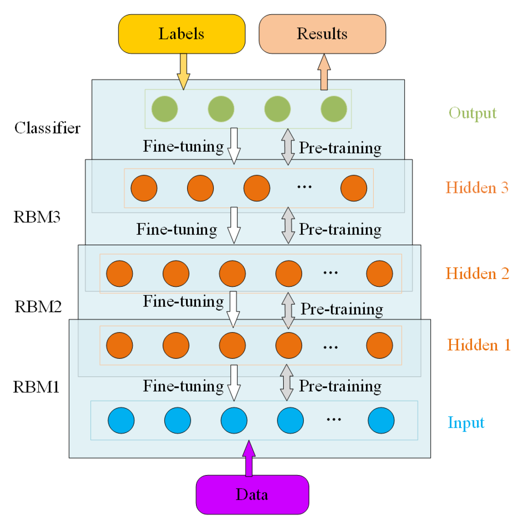
2.2. Structure and Training Process of DBN

DBN is a deep neural network composed of multiple RBMs and a BPNN stack, and BPNN is usually located at the top of the DBN as a supervised learning classifier. The training process of DBN can be divided into two stages: pre-training and fine-tuning. In the pre-training stage, the layer-by-layer greedy algorithm is used to train each RBM in bottom-up order, so that the high-level features of the input data are extracted and the connection weights of the network are updated. In the fine-tuning stage, the BPNN takes the output feature vector of the top-level RBM as input data and continuously optimizes the network parameters in top-down order, in which the label data is used for supervised learning to reduce the loss error and improve the classification accuracy. The training process of DBN consisting of three RBMs is shown in Figure 2.

3. Design of Charging Points Fault Diagnosis

The charging of EVs needs the collaboration of high-power charging equipment and charging points, and Figure 3 shows the relationship between them. The high-power charging equipment is usually connected to multiple charging points to provide stable and reliable voltage and current. Of course, there is also information exchange between them for the respective operating status to ensure the normal charging process. Charging points, as the connection link between high-power charging equipment and EVs, play an important role in charging control and operation as well as billing during the charging process of EVs. Consequently, the following fault diagnosis method for charging points is designed.

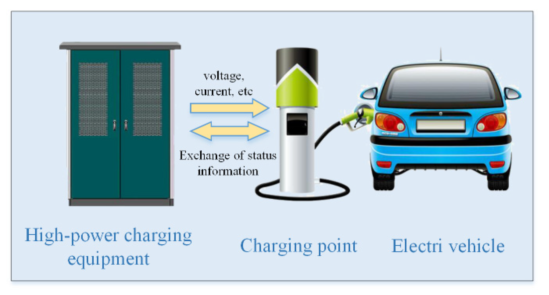
3.1. Fault Characteristics of Charging Points

8 kinds of fault states, as well as normal states of the charging points, are selected as the object of fault diagnosis, and each state is given a different label to distinguish.

Table 1. The fault type of charging points and the fault label.

Description	Symbol	Label
Normal state	d0	0000
Communication failure between EVs and charging points	d1	0001
Insulation testing faults	d2	0010
Charging module output overvoltage	d3	0011
Charging module over-temperature fault	d4	0100
Charging module input phase loss	d5	0101
Battery charging over-current fault	d6	0110
DC bus output over-voltage fault	d7	0111
DC bus output contactor failure	d8	1000

shows the corresponding relationship between them, where d0 is the normal state, and d1–d8 is the fault state.

The occurrence of a fault is related to the change of electrical quantities such as input voltage and input current of charging points. For example, if the charging points do not detect the relevant information of the EVs or the auxiliary power supply of the charging points does not work normally, communication failure between the EVs and charging points may happen. Hence the fault of the charging points can be identified and diagnosed by detecting the change of relevant electrical quantities. The experimental results show that if the 16 parameters, such as input voltage, input current, output voltage, output current, EVs demand voltage, EVs demand current, charging DC bus voltage, AC three-phase voltage Ua, Ub, Uc, battery temperature, battery setting temperature, charging time, insulation detection module state, cooling fan switching state, and auxiliary power module state, are selected as the basis of charging points fault diagnosis, the above-mentioned types of faults can be effectively distinguished.

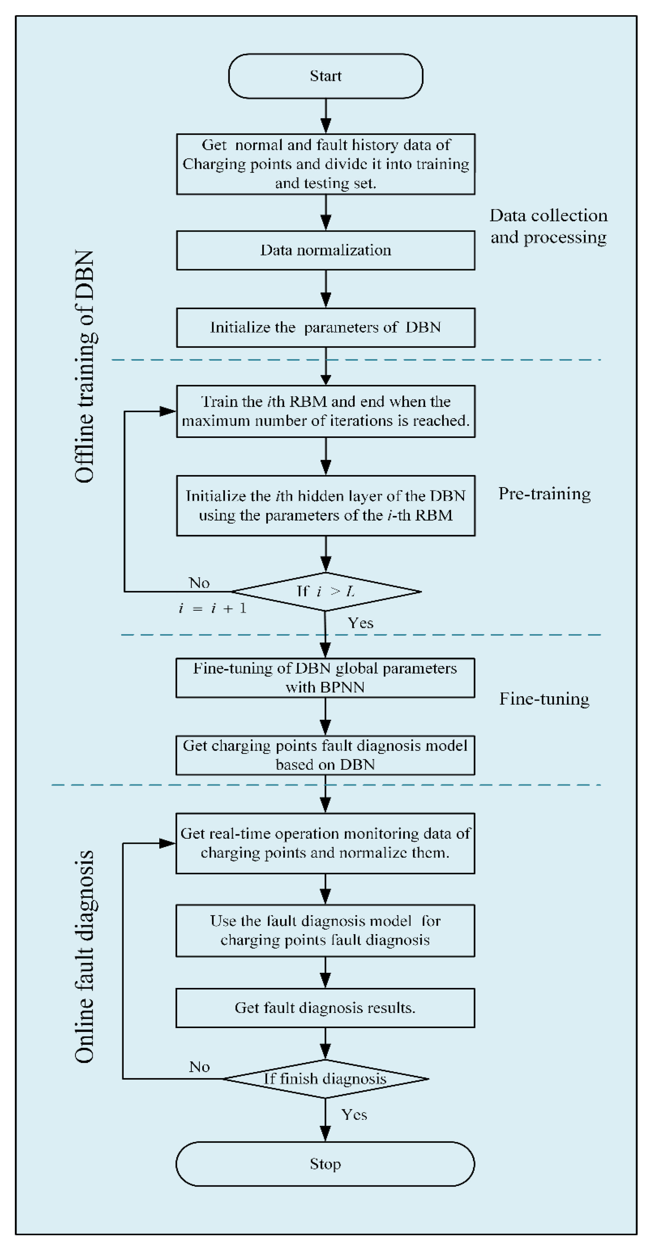
3.2. Design of Fault Diagnosis Flow

The process of fault diagnosis of charging points based on DBN includes two stages: offline training of the DBN fault diagnosis model and online fault diagnosis. The specific process is as follows:

• Organize the historical status data of charging points and build a data set.
• Divide the data set into the training set and test set according to a certain ratio, and normalize them.
• Construct the DBN model through two stages of pre-training and fine-tuning, and optimize the parameters of the DBN model.
• Test the performance of the DBN fault diagnosis model using test data.
• Apply the DBN model that meets the needs of the fault diagnosis of charging points.

Figure 4 shows the realization process in detail.

4. Implementation of Charging Points Fault Diagnosis

4.1. Data Acquisition and Processing

By analyzing the historical status data of charging points, the dataset is available, which contains the normal status and 8 kinds of abnormal status of the charging points, as described in Table 1. Among them, the normal state and each fault state involves 500 data samples, which constitutes a data set containing 4500 samples. The dataset is divided into two parts, a training set containing 80% samples for each state and a test set containing the remaining samples for each state.

To better reflect the data characteristics and improve the convergence speed of the DBN model, it is necessary to normalize the input data. In this paper, we use the method of extreme difference normalization to initialize the data, and the transformation is described as follows:

$$x_{\mathrm{out}}=\frac{x_{\mathrm{in}}-x_{\min }}{x_{\max }-x_{\min }}$$

(13)

where $x_{\max }$ and $x_{\min }$ are the maximum and minimum values of the sample; $x_{\mathrm{out}}$ is the result of normalization of the input data.

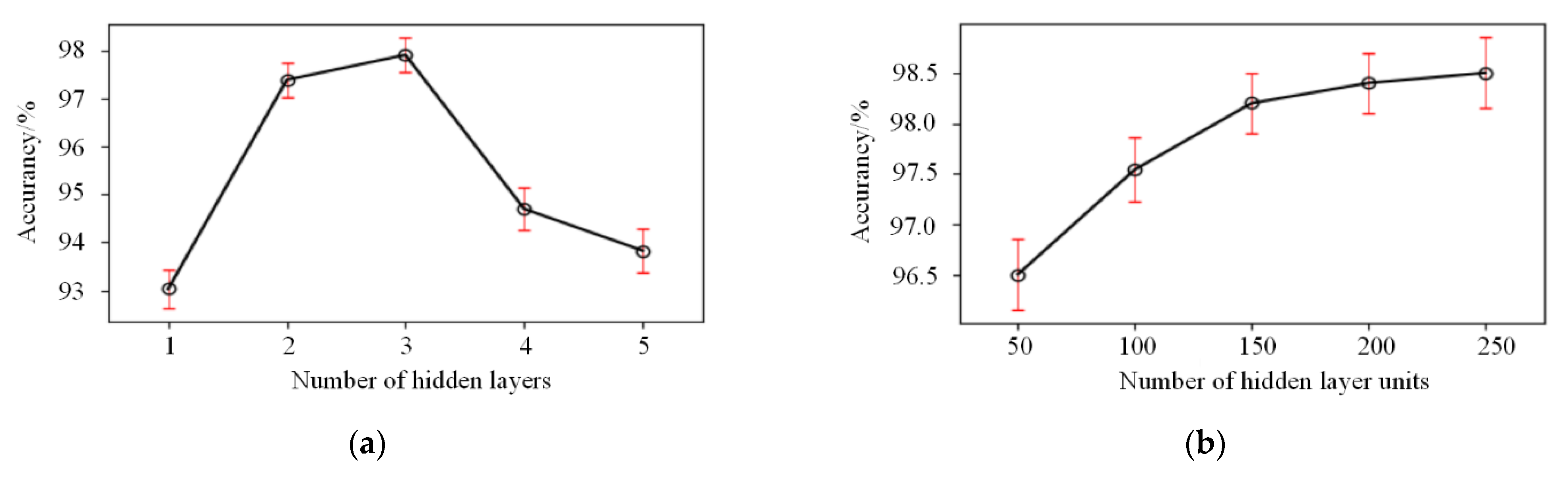
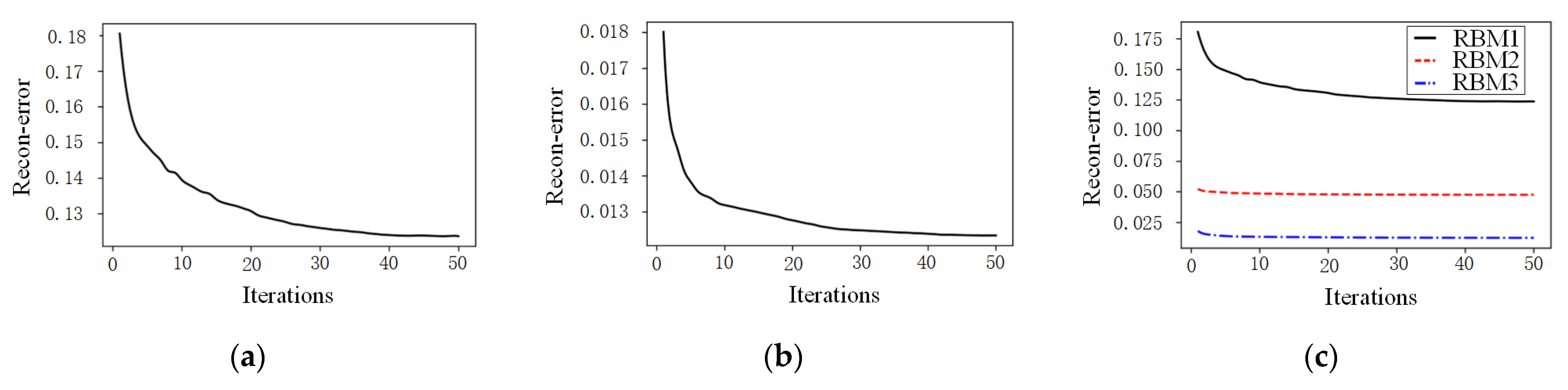
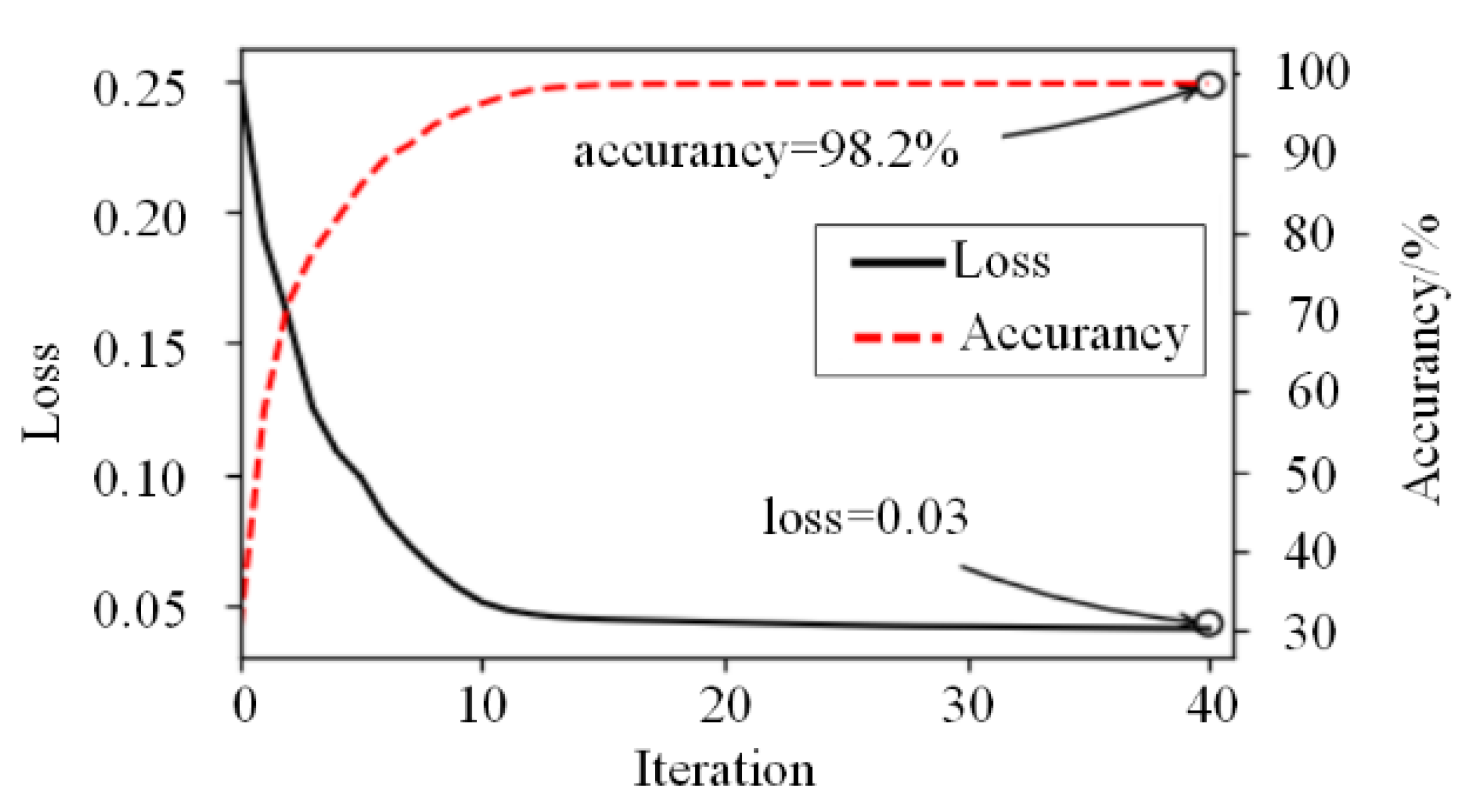
4.2. Experiment and Analysis

The DBN fault diagnosis model is built using Tensorflow, and the experimental software environment is Python3.5.7, Tensorflow1.2.1, the computer hardware configuration for Intel(R) Core (TM) i5-6300HQ CPU @2.30GHz, 8GB of RAM.

Some values of the DBN model are provided in

Table 2. The parameters of DBN.

Description	Symbol	Value
Number of units in input layer	-	16
Number of units in output layer	-	4
Number of iterations of pre-training	n1	50
Number of pre-training batch samples	s1	50
Learning rate of pre-training	a1	0.15
Momentum of pre-training	$\mu$	0.8
Number of iterations of fine-tuning	n2	40
Number of fine-tuning batch samples	s2	20
Learning rate of fine-tuning	a2	0.6

. Moreover, it is necessary to find out the proper number of hidden layers L and units n in the hidden layer. Therefore, we will study the effects of the number of hidden layers and units in the hidden layer on the fault diagnostic accuracy of the charging points with the value determined in Table 2.

The DBN network with L (L = 1, 2, 3, 4, 5) layers is built to test the influence of the number of the hidden layer on the fault diagnostic accuracy. The number of units in each hidden layer is set to 100, and ten trials are carried out with the same data set. The variation of the fault diagnosis accuracy with the number of hidden layers is plotted in an error bar graph, as shown in Figure 5a.

It can be found from Figure 5a that when the accuracy reaches stability, the accuracy and L in the range of L ≤ 3 tend to move together. The highest accuracy is found in L = 3, after which the fault diagnosis accuracy starts to gradually decrease with the increase of L. There are three possible reasons [29]:

• Only the reconstruction errors of the top RBM can reach the preset needs, while the reconstruction errors of the preceding L-1 RBMs are degraded in accuracy by accumulation.
• An increase in the number of hidden layers L leads to excessive error accumulation in the reverse gradient descent algorithm.
• An increase in the number of hidden layers L leads to an effect of increasing the complexity of the running time and decreasing the efficiency.

Figure 5b shows that when the number of hidden layers of the DBN is 3 and the number of hidden layer units is 50–250, the accuracy is above 95%. Meanwhile, with the growth of the number of hidden layer units, the accuracy is increasing. When n is less than 150, the accuracy rises faster. However, the increase in accuracy is less than 0.5% when n is more than 150. Considering the over-fitting problem of the DBM, this paper chooses the network structure with 150 units in the hidden layer.

Reconstruction error (Recon-error) is an important index to evaluate the data feature extraction ability, and the smaller the Recon-error is, the better the data feature mining ability is. Figure 6a shows the Recon-error of the bottom RBM, and Figure 6b shows the Recon-error of the top RBM. Put the Recon-error curves of the three RBMs in one graph, as shown in Figure 6c. The Recon-error of each RBM shows a decreasing trend with the number of iterations as shown in Figure 6, which indicates the data feature extraction ability of each RBM is increasing. The Recon-error of the top RBM reduces to the minimum value of 0.0123 when the number of iterations is 50, now indicating that DBN has strong data feature extraction ability.

Figure 7 visualizes the loss and accuracy of the DBN model in the fine-tuning stage with the number of iterations. The curve shows that the loss error decreases rapidly from 0 to the 10th iteration and gradually tends to a stable value after 20 iterations. Finally, the loss error is 0.03 in 40 iterations when the accuracy of fault diagnosis reaches the maximum value of 98.2% and tends to be stable.

Combining with the above analysis, the structure of DBN is set as 16-150-150-150-4, i.e., the number of hidden layers is 3, and the number of units in the hidden layer is 150. Finally, the detailed recognition results of DBN for the training sample set are shown in Figure 8, where the columns denote the true labels of the data and the rows refer to the predicted ones. From the simulation results, it can be concluded that the DBN with the above structure has better performance in fault diagnosis of charging points.

4.3. Comparison of Methods

To further verify the effectiveness of DBN for fault diagnosis of charging points, it is compared with BPNN, RBFNN, SVM, and CNN in terms of both accuracy and convergence time using the same training and test sets. Each experiment is repeated 10 times to ensure the accuracy of the experimental results, and the average value is taken as the evaluation index. In the experiment, the structure of BPNN is set as 17-9-4, the learning rate is set to 0.05, and the maximum number of iterations is set to 1000. The number of units in each layer of the RBFNN is set to 16-65-4, the learning rate is set to 0.3, and the maximum number of iterations is set to 5000. Gaussian radial basis function is chosen as the kernel function of the SVM, and the penalty factor is set to 1.5. For CNN, depending on the dimensionality of the charging points running data, a one-dimensional convolutional kernel is used. The comparison results are listed in

Table 3. Comparison of results.

Methods	Training Accuracy (%)	Testing Accuracy (%)	Average Accuracy (%)	Convergence Time (s)
BPNN	93.6	92.5	93.05	59.12
RBFNN	95.8	94.7	95.25	24.13
SVM	94.5	93.3	93.90	35.36
CNN	96.3	96.1	96.24	245.74
DBM	98.2	98.1	98.15	206.37

.

According to Table 3, it can be found that the training and testing accuracy of DBN are approximately the same and higher than those of other methods. Conversely, the testing accuracy of the traditional methods has a significant decrease compared with the training accuracy. The results show that the DBN model can better complete the in-depth feature mining of the charging points operating data, so it has greater performance in mapping the relationship between the fault data and the fault type. Moreover, it has better generalization ability. Although CNN also shows good generalization ability, its accuracy is lower than DBN, which indicates that DBN is more adapted to the fault diagnosis of charging points.

From Table 3, we can also find that the CNN model has the longest convergence time and the RBFNN model has the shortest convergence time. There are the following reasons to explain:

• CNN has a more complex structure and training process than other models, and therefore has a significantly longer convergence time.
• RBFNN is a local approximation network, thus the convergence speed is faster.

Although DBN has a long convergence time, similar to CNN, it is acceptable for the fault diagnosis of charging points to obtain higher fault diagnosis accuracy by sacrificing training time.

5. Conclusions

In this paper, a new fault diagnosis method for charging points based on DBN is proposed. As a diagnosis method based on deep learning, the method makes full use of the historical state data of the charging points to obtain the optimal structural parameters of DBN, which improves the fault diagnosis accuracy of charging points without the need to build an accurate mathematical model. To verify the effectiveness of the proposed method, it is compared with the backpropagation neural network, radial basis function neural network, support vector machine, and convolutional neural network. The experimental results show that the proposed method overcomes the defects of traditional fault diagnosis methods such as the weak generalization ability and poor feature extraction ability to a certain extent, and gets better performance in the fault diagnosis accuracy of charging points. From the above conclusions, it can be confirmed that the proposed method is correct and valid, and provides a solution for fault diagnosis of charging points.

References

1. Zhou, D.; Hu, Y. Fault diagnosis techniques for dynamic systems. Acta Autom. Sin. 2009, 35, 748–758. [Google Scholar] [CrossRef]
2. Tidriri, K.; Chatti, N.; Verron, S.; Tiplica, T. Bridging data-driven and model-based approaches for process fault diagnosis and health monitoring: A review of researches and future challenges. Annu. Rev. Control 2016, 42, 63–81. [Google Scholar] [CrossRef]
3. Wu, Y.; Jiang, B.; Shi, P. Incipient fault diagnosis for T–S fuzzy systems with application to high-speed railway traction devices. IET Control Theory Appl. 2016, 10, 2286–2297. [Google Scholar] [CrossRef]
4. Gao, D.; Hou, J.; Liang, K.; Yang, Q. Fault diagnosis system for electric vehicle charging devices based on fault tree analysis. In Proceedings of the 2018 37th Chinese Control Conference (CCC), Wuhan, China, 25–27 July 2018; pp. 5055–5059. [Google Scholar]
5. Liu, X.; Han, J.; Wei, X.; Zhang, H.; Hu, X. Distributed fault detection for non-linear multi-agent systems: An adjustable dimension observer design method. IET Control Theory Appl. 2019, 13, 2407–2415. [Google Scholar] [CrossRef]
6. Zhong, Y.; Zhang, W.; Zhang, Y.; Zuo, J.; Zhan, H. Sensor fault detection and diagnosis for an unmanned quadrotor helicopter. J. Intell. Robot. Syst. 2019, 96, 555–572. [Google Scholar] [CrossRef]
7. Rahimi, A.; Kumar, K.D.; Alighanbari, H. Fault estimation of satellite reaction wheels using covariance based adaptive unscented Kalman filter. Acta Astronaut. 2017, 134, 159–169. [Google Scholar] [CrossRef]
8. Wang, H.L.; Zhou, G.B. State of charge prediction of supercapacitors via combination of Kalman filtering and backpropagation neural network. IET Electr. Power Appl. 2018, 12, 588–594. [Google Scholar]
9. Ahmed, R.; El Sayed, M.; Gadsden, S.A.; Tjong, J.; Habibi, S. Automotive internal-combustion-engine fault detection and classification using artificial neural network Techniques. IEEE Trans. Veh. Technol. 2015, 64, 21–33. [Google Scholar] [CrossRef]
10. Ji, Z.; Liu, W. Open-circuit fault detection for three-phase inverter based on backpropagation neural network. Neural Comput. Appl. 2018, 31, 4665–4674. [Google Scholar] [CrossRef]
11. Chen, Y.; Ma, H.W.; Dong, M. Automatic classification of welding defects from ultrasonic signals using an SVM-based RBF neural network approach. Insight 2018, 60, 194–199. [Google Scholar] [CrossRef]
12. Liu, L.; Ji, Y.F.; Gao, Y.; Kuang, L. Classification of epileptic electroencephalograms signal based on integrated radius-basis-function neural-network. J. Med. Imaging Health Inform. 2018, 8, 1462–1467. [Google Scholar] [CrossRef]
13. Zhou, W.; Li, X.; Yi, J.; He, H. A novel UKF-RBF method based on adaptive noise factor for fault diagnosis in pumping unit. IEEE Trans. Ind. Inform. 2019, 15, 1415–1424. [Google Scholar] [CrossRef]
14. Wang, Z.H.; Shen, Y.; Zhang, X.L. Actuator fault estimation for a class of nonlinear descriptor systems. Int. J. Syst. Sci. 2014, 45, 487–496. [Google Scholar] [CrossRef]
15. Konar, P.; Chattopadhyay, P. Bearing fault detection of induction motor using wavelet and Support Vector Machines (SVMs). Appl. Soft. Comput. 2011, 11, 4203–4211. [Google Scholar] [CrossRef]
16. Yan, X.; Jia, M. A novel optimized SVM classification algorithm with multi-domain feature and its application to fault diagnosis of rolling bearing. Neurocomputing 2018, 313, 47–64. [Google Scholar] [CrossRef]
17. Zidi, S.; Moulahi, T.; Alaya, B. Fault Detection in wireless sensor networks through SVM classifier. IEEE Sens. J. 2018, 18, 340–347. [Google Scholar] [CrossRef]
18. Wen, L.; Li, X.Y.; Gao, L.; Zhang, Y.Y. A new convolutional neural network-based data-driven fault diagnosis Method. IEEE Trans. Ind. Electron. 2018, 65, 5990–5998. [Google Scholar] [CrossRef]
19. Du, T.; Zhang, H.; Wang, L. Analogue circuit fault diagnosis based on convolution neural network. Electron. Lett. 2019, 55, 1277–1278. [Google Scholar] [CrossRef]
20. Xia, M.; Li, T.; Xu, L.; Liu, L.Z.; de Silva, C.W. Fault diagnosis for rotating machinery using multiple sensors and convolutional neural networks. IEEE-ASME Trans. Mechatron. 2018, 23, 101–110. [Google Scholar] [CrossRef]
21. Ren, H.; Qu, J.; Chai, Y.; Tang, Q.; Ye, X. Deep learning for fault diagnosis: The state of the art and challenge. Control Decis. 2017, 32, 1345–1358. [Google Scholar]
22. Deng, L.; Hinton, G.E.; Kingsbury, B. New types of deep neural network learning for speech recognition and related applications: An overview. In Proceedings of the IEEE International Conference on Acoustics, Speech, and Signal Processing (ICASSP), Vancouver, BC, Canada, 26–31 May 2013; pp. 8599–8603. [Google Scholar]
23. Chen, Z.; Li, W. Multisensor feature fusion for bearing fault diagnosis using sparse autoencoder and deep belief network. IEEE Trans. Instrum. Meas. 2017, 66, 1693–1702. [Google Scholar] [CrossRef]
24. Yu, D.; Chen, Z.M.; Xiahou, K.S.; Li, M.S.; Ji, T.Y.; Wu, Q.H. A radically data-driven method for fault detection and diagnosis in wind turbines. Int. J. Electr. Power Energy Syst. 2018, 99, 577–584. [Google Scholar] [CrossRef]
25. Li, M.; Yu, D.; Chen, Z.; XiaHou, K.; Li, Y.; Ji, T. Fault diagnosis and isolation method for wind turbines based on deep belief network. Electr. Mach. Control 2019, 23, 114–122. [Google Scholar]
26. Zhu, J.; Hu, T.; Jiang, B.; Yang, X. Intelligent bearing fault diagnosis using PCA–DBN framework. Neural Comput. Appl. 2019, 32, 10773–10781. [Google Scholar] [CrossRef]
27. Fischer, A.; Igel, C. Training restricted boltzmann machines: An introduction. Pattern Recognit. 2014, 47, 25–39. [Google Scholar] [CrossRef]
28. Hinton, G.E. Training products of experts by minimizing contrastive divergence. Neural Comput. 2002, 14, 1771–1800. [Google Scholar] [CrossRef] [PubMed]
29. Pan, G.; Chai, W.; Qiao, J. Calculation for depth of deep belief network. Control Decis. 2015, 30, 256–260. [Google Scholar]
Figure 1. Structure of RBM.
Wevj 12 00047 g001
Figure 2. Structure and training process of DBN.
Wevj 12 00047 g002
Figure 3. The relationship between high-power charging equipment, DC charging points, and EVs.
Wevj 12 00047 g003
Figure 4. Fault diagnosis flow based on DBN.
Wevj 12 00047 g004
Figure 5. Fault diagnosis accuracy of DBN with the different number of hidden layers and number of units in the hidden layer. (a) Accuracy of DBN with different hidden layers. (b) Accuracy of DBN with different hidden units.
Wevj 12 00047 g005
Figure 6. Recon-error of different RBM. (a) Recon-error of the bottom RBM. (b) Recon-error of the top RBM. (c) Recon- errors of three-layer RBMs.
Wevj 12 00047 g006
Figure 7. The change curve of DBN loss value and accuracy.
Wevj 12 00047 g007
Figure 8. The details of the proportion of samples in each fault divided into other category.
Wevj 12 00047 g008